Abstract
HURLEY, FORREST JAMES. Effects of Powdered Kenaf Addition on the Performance of Lab-Scale Activated Sludge Reactors. (Under the direction of Dr. F.L. de los Reyes III.)
The effects on wastewater treatment due to addition to mixed liquor (ML) of a fine lignocellulosic powder made of dried kenaf (plant) were assessed using lab-scale sequencing batch reactors (SBRs) designed for enhanced biological nitrogen and phosphorus removal and treating real municipal wastewater. Removal of organic carbon, nitrogen, phosphorus and suspended solids at various aeration intensities were compared between kenaf treatment and control SBRs. Mixed liquor concentrations, adsorption of heavy metals, sludge settling characteristics and microbial kinetics of the treatment reactor were also compared to those of the control SBR, which received no kenaf.
No significant effects on carbon, phosphorus or suspended solids removal were detected. There was a small increase in mixed liquor suspended solids (MLSS) and mixed liquor volatile suspended solids (MLVSS) with kenaf treatment, possibly more than the accumulated mass of kenaf. Nitrogen removal was unaffected by the treatment when aeration intensity was near optimum, which for these SBRs was an aeration ratio (AR) of roughly 11, where the AR is defined as the mass of O2 supplied to the SBR each cycle, divided by the mass of COD exerted per cycle. However, the kenaf supplemented ML removed nitrogen significantly (alpha = 0.01) better than the control when the AR was below the ideal range, suggesting that full-scale wastewater treatment plants (WWTPs)
Effects of Powdered Kenaf Addition on the Performance of Lab-Scale Activated Sludge Reactors
by
Forrest James Hurley
A thesis submitted to the Graduate Faculty of North Carolina State University
in partial fulfillment of the requirements for the Degree of
Master of Science
Environmental Engineering
Raleigh, North Carolina 2013
APPROVED BY:
______________________ _______________________
Dr. Detlef Knappe Dr. Tarek Aziz
ii Dedication
To my wife and sons.
iii Biography
iv
Acknowledgments
v
Table of Contents
List of Tables ………. vii
List of Figures ………. viii
Introduction ………. 1
Materials and Methods ……….. 6
Reactor Design ……….. 6
Computer Modeling ……….. 8
Lab-Scale Reactors ……….. 18
Feedstocks ……….. 21
Collection of Samples ……….. 24
Analysis of Samples ……….. 27
Results ………. 37
Effluent total and volatile suspended solids ……….. 37
Mixed Liquor Suspended Solids and Volatile Suspended Solids 42
Sludge Volume Index ……….. 47
Heavy Metals ……….. 49
Floc Size ……….. 56
Chemical Oxygen Demanded ……… 60
Nitrogen species ……….. 65
Total Phosphate ……….. 77
Intra-Cycle Samples ……….. 78
Batch reactor tests ……….. 83
vi
Future Work ………. 88
References ………. 89
Appendices ………. 91
Appendix 1 ……….. 92
Appendix 2 ……….. 93
Appendix 3 ……….. 94
Appendix 4 ……….. 96
Appendix 5 ……….…. 98
vii List of Tables
Table 2.1 Measured influent wastewater characteristics ……… 9
Table 2.2 Estimated ASIM input values for influent wastewater 11 Table 2.3 SBR treatment cycle used for ASIM and benchtop models 12 Table 2.4 Annual average influent characteristics at NCWRF 22 Table 2.5 Hach colorimetric Test-N-Tube kits ……….. 34
Table 3.1 Mean suspended solids in mixed liquor ……….. 43
Table 3.2 Pearson Product-Moment Correlation Coefficients 44 Table 3.3 Summary of SVI statistics ………. 47
Table 3.4 Mean metals concentrations ………. 50
Table 3.5 Summary of COD statistics ………. 61
Table 3.6 Linear correlation coefficients ………. 63
Table 3.7 Effluent Total Nitrogen summary statistics ……… 66
Table 3.8 Percent removal of Total Nitrogen ……….. 67
Table 3.9 Effluent ammonia-nitrogen concentrations ……… 72
viii List of Figures
Figure 1.1 Nearly mature kenaf ……… 3
Figure 1.2 Harvesting mature kenaf ……… 4
Figure 1.3 Powdered dried kenaf ……….. 4
Figure 2.1 Ammonium concentration within reactor ………. 13
Figure 2.2 Soluble substrate concentration within reactor ………. 14
Figure 2.3 Typical actual DO concentration in the reactors ………….. 15
Figure 2.4 Nitrate concentration within reactor ……….. 16
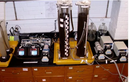
Figure 2.5 Benchtop setup ………. 20
Figure 3.1 Effluent total suspended and volatile suspended solids 39
Figure 3.2 Total Suspended Solids concentrations ……….. 39
Figure 3.3 Volatile Suspended Solids concentrations ……… 40
Figure 3.4 Percent removal of TSS ………. 41
Figure 3.5 Mixed liquor suspended and volatile suspended solids 43
Figure 3.6 Regression on kenaf and control SBRs’ MLSS ……… 45
Figure 3.7 Regression on kenaf and control SBRs’ MLVSS ……… 46
Figure 3.8 Sludge volume index of kenaf and control mixed liquors 48
Figure 3.9 Arsenic concentrations in dried sludge solids ……… 51
Figure 3.10 Copper concentrations in dried sludge solids ……… 51
Figure 3.11 Lead concentrations in dried sludge solids ……… 52
Figure 3.12 Selenium concentrations in dried sludge solids …………... 53
Figure 3.13 Cadmium concentrations in dried sludge solids ……… 53
ix
Introduction
Costs associated with waste sludge processing and disposal are a major operating expense for most municipal wastewater treatment plants [1], as are those for energy for aeration needed for carbon removal (expressed as chemical oxygen demand, COD) and nitrification. Additionally, many plants may face penalties for non-compliance with their discharge permits, which have become more restrictive over time. If reduced aeration or enhanced nitrogen and COD removal and
improvements in sludge settling characteristics could be accomplished without major changes to the physical plant, operating costs could be lower and compliance with environmental standards more likely.
One common strategy to improve plant performance has been to retrofit suspended growth systems with submerged surface area for attached growth of biofilms. Conventional and enhanced Activated Sludge (AS) systems use complete mixing to maximize contact between suspended microbes and their growth substrates, thus optimizing removal of those substrates. But for some microbes, attached growth may have advantages such as microenvironments that can form within biofilms. For example an anoxic zone in a biofilm exposed to aerated WW may facilitate
2
IFAS plants may be able to carry a higher biomass concentration in the reactor because the attached fraction of the biomass does not contribute much to clarifier loading. More biomass can allow the plant to support higher organic loading or to achieve more complete removal if it is already
overloaded. Because the attached biomass never leaves the reactor, the mean solids retention time (SRT) is longer than that of a hydraulically similar conventional system and so yield is lower and there is less excess sludge production. The increased SRT for attached microbes especially benefits the slow growing nitrifiers. More stable output under varying loads than in conventional systems and improved sludge settling have also been observed in IFAS plants [2]. Plastic media with a rough surface, freely circulating in the mixed liquor can encourage biofilm development, but may
necessitate modifications to the plant such as a downstream screen to retain the media. Stationary racks of long fibers for mixed liquor to flow through have also been successful, but require
maintenance and may change the plant’s hydraulics [3].
3
sludge systems is reported by its manufacturer to provide freely circulating submerged surface area (7.4 m2/gram, as measured by BET isotherms) for formation of robust biofilms. The claim is that this results in better COD and nitrogen removal with less aeration as well as enhanced sludge settling and lower sludge disposal volume; and all with no need for media maintenance or recovery or for plant modifications (http://rfwastewater.com/). These claims are based on the company’s trials at several full scale WWTPs and have yet to be independently verified in well controlled published studies.
4
Figure 1.2: Harvesting mature kenaf. (Agricultural Marketing Resource Center)
5
The objectives of this study were to evaluate the effects of powdered kenaf addition on bulk process parameters of lab scale WWTPs performing biological nitrogen and phosphorus removal. Removal of COD, nitrogen, phosphorus and suspended solids at various aeration intensities were compared between kenaf treated and control bioreactors. Mixed liquor suspended solids and volatile suspended solids (MLSS, MLVSS) were tracked to determine whether changes in influent strength and aeration intensity affected the growth of the microbial cohorts of the systems similarly.
Sludge settling characteristics of the bioreactors were quantified by use of the Sludge Volume Index (SVI) which is calculated by dividing the 30 minute settled sludge volume (SSV30) in mL/L by the MLSS in g/L, resulting in units of mL/g. SVI can be interpreted as the volume occupied by each dry gram of settled sludge solids. Values of SVI greater than 150 mL/g are considered to be indicative of poor sludge settling characteristics while those below 80 mL/g represent sludges with excellent settling characteristics [11]. Distributions of the particle sizes in mixed liquor solids samples were compared in order to elucidate the mechanisms behind any significant differences in SVI.
Differences in the concentrations of heavy metals in dried sludge solids samples from each
bioreactor identified elements which tend to adsorb to the kenaf. Lee and Rowell [8] found that of the 5 types of plant fibers they tested, kenaf had the best ability to remove copper, nickel and zinc ions from solution. While removal of heavy metals from the liquid waste stream is desirable, their accumulation in the solids they adsorb to could limit waste sludge disposal options.
The microbial kinetics of each bioreactor’s cohort were assessed by batch reactor testing samples of mixed liquor (ML) borrowed from the kenaf treated and control systems, and by intensive in situ
6
Materials and Methods
Reactor Design
Laboratory scale sequencing batch reactors (SBRs) were chosen to model the continuous flow systems typical of full scale wastewater treatment plants (WWTPs). While wastewater and biomass encounter different environmental conditions at different locations in continuous systems, in an SBR the same performance can be achieved by changing the conditions over time in a single tank. This is accomplished by operating an SBR in a repeating cycle of phases, each with its own environmental regime. At its simplest, an SBR’s cycle consists of a fill phase in which influent wastewater is added to the reactor, a react phase during which biological action transforms problematic constituents in the wastewater, a settle phase to separate solids (including biomass) from the bulk liquid, and a decant phase to remove treated clarified effluent. The react portion of the cycle can be divided into several phases, each with unique environmental conditions and a unique duration. In continuous flow systems the amount of time spent in each treatment stage (for a given flowrate) is determined by tank volume, which is difficult to alter experimentally. However in an SBR, timer settings (which are easy to change) control the duration of each process. The flexibility to alter the length of any phase and even the order of the react phases allows the SBR to simulate the performance of almost any type of WWTP, as long as the systems have comparable mean solids residence times (SRT). [11]
7
8 Computer Modeling
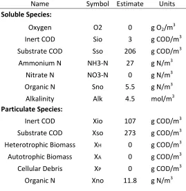
The treatment cycle for this study was developed with the aid of ASIM modeling software implementing ASM No. 1 in SBR mode. Computer modeling allows many process options to be evaluated quickly. By testing various durations for each treatment phase, the performance of the SBR cycle can be optimized (for a particular wastewater and flow regime). The downside of ASIM (and many computer models) is that it requires inputs of influent constituent species to be in non-overlapping categories or partitions so that the materials mass balances can be solved, rather than using conventional lumped parameters such as MLSS or total COD [12]. Such data is not usually available for a particular wastewater, so it becomes necessary to estimate the ASIM inputs from existing data. A limited dataset (Table 2.1) characterizing the influent wastewater at a local WWTP (one of two which were being considered at the time for wastewater collection for this study’s feedstock) served as the basis for estimating the ASIM inputs used for this model. Those influent parameters were then held constant through each model run, rather than varying weekly as the physical bench-top model’s feedstock did.
9
biodegradable portions of the tCOD must be further subdivided into solid and soluble fractions based on available solids data.
Table 2.1: Measured influent wastewater characteristics at Triangle WWTP, Durham Co., NC
Date BOD5 NH3 Total N TSS Total P
May 2010 324 37.5 54.8 347 8.93
Aug 2010 241.3 31 40.7 248.2 6.93
Nov 2010 278.3 28.7 37 250.5 5.22
Feb 2011 278.5 33.5 44.3 238.2 5.93 Average 280.53 32.68 44.20 270.98 6.75
S.D. 33.85 3.77 7.67 50.96 1.61
C.V. 0.12 0.12 0.17 0.19 0.24
The solids dataset includes only values for TSS, but the wastewater was reported to be higher in fixed suspended solids (FSS) than average (due to some industrial customers), with only about 70% of TSS volatilizing. Therefore the volatile suspended solids (VSS) in COD concentration units was estimated as VSS = 0.7 mg VSS/mg TSS * 1.41 mg COD/ mg VSS * 271 mg TSS /L = 267 mg COD/L. It was assumed that the particulate organic matter (represented by VSS) is 35% to 40%
10
COD, Sso, was assumed to be approximately 43% of the biodegradable COD, or 206 mg COD/L. The remaining biodegradable COD is particulate, Xso, which is 273 mg COD/L.
Ammonia concentration for this wastewater was converted to ammonia-N concentration by
multiplying 33 mg NH3 by 14.01 mg N/17.03 mg NH3 = 27 mg N/L. Concentrations of nitrite nitrogen and nitrate nitrogen in municipal wastewater are typically insignificant, so they were assigned a value of zero. The organic nitrogen was then found by subtracting the ammonia nitrogen from the total nitrogen: Norg = TN – NH3-N = 17 mg N/L. Just as with tCOD, organic nitrogen must be partitioned into particulate and soluble fractions, each of which has inert and substrate
11
Table 2.2: Estimated ASIM input values for influent wastewater
Name Symbol Estimate Units Soluble Species:
Oxygen O2 0 g O2/m3
Inert COD Sio 3 g COD/m3
Substrate COD Sso 206 g COD/m3 Ammonium N NH3-N 27 g N/m3
Nitrate N NO3-N 0 g N/m3
Organic N Sno 5.5 g N/m3
Alkalinity Alk 4.5 mol/m3 Particulate Species:
Inert COD Xio 107 g COD/m3
Substrate COD Xso 273 g COD/m3 Heterotrophic Biomass XH 0 g COD/m3
Autotrophic Biomass XA 0 g COD/m3
Cellular Debris XP 0 g COD/m3
Organic N Xno 11.8 g N/m3
12
process, except that because SBRs do not permit true internal mixed liquor recycle there is no need for the first anoxic stage. The SBR cycle used in this study is presented in Table 2.3.
Table 2.3: SBR treatment cycle used for both ASIM and benchtop models
Phase Duration Mixer Volume In/Out
(min.s)
Fill 5 none +1500mL WW +167mL DI [+ kenaf]
Anaerobic 50 recirculation
Aerobic 70 aeration
Anoxic 85 recirculation
Air Strip 5 aeration -167mL biomass waste
Settle 20 none
Decant 5 none -1500mL effluent
13
The first react phase, which was anaerobic, was designed to facilitate the fermentation of some organic carbon to acetate as well as the ammonification of organic nitrogen. As shown by the ASIM output in Figure 2.1, 50 minutes duration for this phase was just long enough for the ammonia concentration to reach a plateau in the ASIM model. In the physical bench-top model however, most fermentation and ammonification probably occurred in the feedstock tank, before the wastewater entered the reactor. This phase did still function well in the bench-top model as an anaerobic selector benefiting phosphate accumulating organisms (PAOs). Phosphate removal is not supported in ASM No. 1, therefore this process was not modeled in ASIM.
Figure 2.1: Ammonium concentration within reactor through 1 four hour cycle
1st React Phase
ANA
2nd React Phase
14
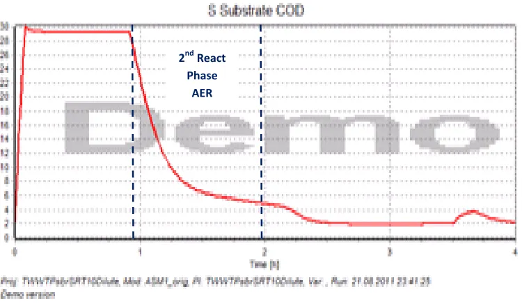
The second react phase was aerobic. It was designed to last long enough for essentially all of the ammonia to be converted to nitrate by nitrifying bacteria (AOB and NOB) while most of the organic carbon (i.e. COD) is oxidized to carbon dioxide (Figure 2.2). It is important to not allow all of the COD to be consumed during this phase because some will be needed as substrate for the heterotrophic denitrifiers in the subsequent anoxic treatment phase.
Figure 2.2: Soluble substrate concentration within reactor through 1 four hour cycle
In the ASIM model the dissolved oxygen concentration (DO) was assumed to remain constant at 2.0 mg/L throughout this aerobic phase (and the brief re-aeration phase later in the cycle), while in all non-aerated phases the DO was equal to 0.0 mg/L. In the physical bench-top model, however, the
2nd React Phase
15
DO varied continuously, often reaching its peak value only near the end of the primary aeration phase, then declining through the first 10 to 30 minutes of the next phase. Figure 2.3 shows the actual DO concentration in the control reactor through a typical cycle. Dissolved oxygen
concentrations in the experimental reactor were similar.
Figure 2.3: Typical actual DO concentration in the reactors
The third react phase was anoxic and had the longest duration in order to allow time for the facultative denitrifiers to convert nitrate from the previous phase to nitrogen gas which then exits the system (Figure 2.4).
16
phases to inhibit further denitrification (which could otherwise lead to rising sludge during clarification.) Residual DO in the settle and decant phases was also important to prevent the anaerobic conditions that cause PAOs to release all of their stored phosphate back into solution.
Figure 2.4: Nitrate concentration within reactor through 1 four hour cycle
The outputs from an ASIM model run, like the inputs, also require some interpretation and conversion in order to be able to compare them with common measurements. For instance, the effluent soluble COD can be predicted by aggregating the values for inert and substrate soluble COD: sCOD = Ss + Si. ASIM assumes a perfect clarifier in which no solids remain in the effluent, so the effluent tCOD would be equal to the sCOD. However, in physical reactors and full scale WWTPs,
2nd React Phase
AER
3rd React Phase
17
clarification is never perfect. With no ability to partition the solids into those that settle well and those that do not, there is no way to predict the effluent tCOD from ASIM output. Mixed liquor suspended solids (MLSS, in COD units) can be estimated by summing the particulate substrate and inert COD, Xs and Xi, the heterotrophic and autotrophic biomass, XH and XA, and the cellular debris,
Xp. The result can be converted to conventional mass units by dividing by 1.2 mg COD/mg TSS. Determining the volatile suspended solids, MLVSS, is more problematic and requires some
18 Lab-Scale Reactors
Two identical 10.0 L reactors were fabricated from clear acrylic which is stronger than Plexiglas and less prone to pitting by attached microbes. Acrylic is also more transparent than plexiglas and therefore permits better observation of the tank’s contents. This proved useful in detecting zones of inadequate mixing and in monitoring and removing attached growth from the reactor walls. A dimensioned drawing of the reactors can be found in Appendix 1.
Four 2 channel peristaltic pumps transferred liquids into or out of the reactors. A schematic of the benchtop setup is shown in Appendix 2. Referring to that illustration, all pumps with a letter designation are peristaltic while those with numbers are centrifugal. Pump A was a Cole-Parmer Masterflex L/S model 7554-90 which delivered 167 mL of either DI water (control SBR) or a
suspension of kenaf powder in DI water (experimental SBR) to the reactors during the 5 minute Fill phase. Pump B, a Cole-Parmer model 7553-02, was responsible for feeding 1500 mL of wastewater to the reactors in the same 5 minutes. Pump C, a Cole-Parmer model 7554-90, removed 1500 mL of treated effluent in the Decant phase. Biowastage occurred in the re-aeration phase (React Phase 4) when Pump D, a Cole-Parmer model 7553-30, removed 167 mL of mixed liquor in 2 minutes.
19
and 3 was upward, with return mixed liquor entering near the bottom of the tank then exiting the reactor at the pump intake located approximately 0.1 m below the free surface. Air was supplied to the reactors in the aerated phases (React Phases 2 and 4) by a vacuum/air pump which was
connected to Cole-Parmer acrylic variable area airflow meters with direct reading scales from 0.04 to 0.5 LPM and brass needle valve regulators, then anti-siphon check valves and finally to 3 inch disk shaped air stone diffusers placed in the bottom of each reactor.
All pumps and mixers were controlled by 2 ChronTrol XT Series timers, each capable of switching 4 separate 120 v electrical circuits on and off multiple times in each SBR cycle.
20
21 Feedstocks
Many lab scale wastewater treatment studies utilize synthetic wastewater as feedstock because its constituents can be fully controlled and characterized analytically, with little or no need for testing, and because it is easy to procure, typically by mixing measured masses of a fairly small number of chemical species with DI water right in the lab as needed. For this study, there was concern that synthetic WW would not adequately model the diversity or the variability of substrates influent to biological treatment at municipal WWTPs, and therefore might select for a substantially less diverse (and less robust) microbial cohort than would be found at a real treatment plant. To more ably apply plant performance and microbial kinetics results from the lab scale reactors to full scale WWTPs, it was decided to feed real municipal wastewater.
Municipal wastewater for feedstock was collected weekly from the North Cary Water Reclamation Facility in North Carolina which treats an average of 7 million gallons a day generated by 60,000 residents and several industries. The plant’s reported average influent characteristics for one year (9/1/2010-8/31/2011) are given in Table 2.4.
Wastewater feedstock was transferred from the final tank of the headworks by a submersible centrifugal pump which was placed 0.3 – 0.5 m below the surface. The wastewater in this tank had already undergone primary treatment of band screening and grit and FOG removal. Further physical treatment (necessitated by tubing clogs in the lab) was carried out during the collection procedure by passing the wastewater through a sieve (ASTM No. 16), which probably removed some
22
process. The feedstock was transported and stored in sealed polypropylene barrels. Any feedstock which would not be used within 48 hours was held at 4°C until needed.
Table 2.4: Annual average influent characteristics at NCWRF
Species Concentration
pH 7.44
VSS 330 mg/L TSS 360 mg/L COD 569 mg/L CBOD 261 mg/L P 6.53 mg/L TKN 44.6 mg/L NH3 31.0 mg/L NO3 1.70 mg/L Alk 183 mg/L
Both reactors were seeded with 10.0 L fresh return activated sludge from the North Cary plant. They were initially operated under identical conditions, being fed only 90% wastewater and 10% DI water (no kenaf) until they reached a stable state and were well matched in terms of performance. With a 10 day SRT and influent qualities that changed every 7 days, achieving a true steady state was impossible, just as it is at real WWTPs.
23
cycle was constant (1/6 L), but the dry mass of kenaf in that volume was adjusted weekly according to a dosage formula provided by the manufacturer (personal correspondence, Walt Brown,
RFWastewater, 2011). The control reactor received the same volume of DI water without kenaf in order to control for dilution.
The daily dose of kenaf required for biofilm development depended on the daily load of BOD (assumed to be 80% of COD) and of total Nitrogen (TN). Loading varied weekly with each new batch of wastewater feedstock. Other dosage formula inputs were held constant. These included: the BOD removal rate (RBOD = 4.5 g/m2day), the total nitrogen removal rate (RTN = 0.125 g/m2day), mean
solids retention time (SRT = 10 days), the surface area of kenaf powder (SAk) which was determined
by BET isotherms to be 7.4 m2/g, and a daily loss factor to account for chemical oxidation and microbial catabolism of the kenaf. Initially the daily loss factor was taken to be 1.25 as
24 Collection of Samples
In order to test the wastewater feedstock for concentrations of total and volatile suspended solids (TSS and VSS), COD, Total Nitrogen (TN), ammonia nitrogen (NH3-N), nitrite nitrogen (NO2-N), nitrate
nitrogen (NO3-N) and Total Phosphate (TPO4), samples were acquired by thoroughly mixing the
wastewater then siphoning approximately 1500 mL into a 2.0 L Erlenmeyer flask. The mouth of the flask was sealed with parafilm. Due to time constraints, not all testing of the sample could be carried out immediately. Any unused sample was held at 4°C until analysis was complete.
Effluent concentrations of the same species as in the wastewater feedstock were also assessed. Samples from each reactor were collected by diverting the appropriate tubing from the waste effluent tank to separate 2.0 L Erlenmeyer flasks. Each flask received the entire 1500 mL of treated effluent which was pumped out of the reactor at the end of a single cycle. Effluent tubing was then returned to the waste barrel, and the flasks were sealed with parafilm. The actual volume of effluent in each flask was observed to ensure that the peristaltic pump was functioning according to design. Analysis of effluent samples was generally performed immediately after collection.
25
Samples of settled sludge were gathered from each SBR to determine the concentrations of arsenic, cadmium, chromium, cobalt, copper, lead, nickel, selenium and zinc in the sludge solids. Up to two days of biowaste from each reactor was allowed to accumulate in 2.0 L graduated cylinders. Approximately 1800 mL of clear supernatant could then be pumped out of the graduated cylinders leaving 180 to 200 mL of settled sludge which was retained for drying. The sludge was placed in crucibles and dewatered at 90°C for at least 2 days before being dried at 105°C for 1 day. The dry solids were scraped out of the crucibles with a glass rod and put into 15 mL centrifuge tubes. With lids loose, the tubes and their solids were held at 105°C for 1 hour. The lids were then tightened while still warm. The dried solids were stored in the sealed centrifuge tubes in the dark at room temperature until they were analyzed.
Mixed liquor samples for DNA extraction, floc particle size distribution (PSD) measurement and fluorescence in situ hybridization (FISH) were collected using a clean catch technique during the two minutes of regularly scheduled biowaste removal in the re-aeration phase of the SBR cycle. For the first 30 seconds of waste pump run time the mixed liquor was allowed to flow into the usual
26
biomass pellets frozen at -60°C for future molecular analysis. The fourth tube from each reactor provided ample mixed liquor for fixing of FISH samples and for plating for floc particle size surveys.
Changes in soluble species (sCOD, sTN, sNH3-N, NO2-N, NO3-N) concentrations throughout individual
cycles were tracked by intensively sampling the in situ ML of the mature reactors. On two
consecutive days, 24 samples of 15 mL of mixed liquor were collected from each of the reactors in one 4 hour cycle. Samples were removed from both SBRs simultaneously using 60 mL syringes inserted 2-3 cm below the free surface. Around 25 mL was withdrawn from each tank then 15 mL of that was ejected into 15 mL centrifuge tubes. Whatever ML remained in the syringe was
27 Analysis of Samples
All suspended solids measurements, whether for the wastewater feedstock, the mixed liquor or the effluent, were accomplished by the same method which began by placing an appropriate number of clean crucibles and 55 mm glass microfiber filters in a 550°C furnace for at least 15 minutes. The filters and crucibles were then carefully removed from the furnace with long handled tongs and allowed to cool to room temperature. Only clean gloves or tongs were used to handle the crucibles and filters from this point on to avoid transfer of oils from the skin or other materials from
contaminated gloves. Each crucible and filter combination was weighed and the mass recorded. A Buchner funnel was inserted into a side arm flask connected to a vacuum pump. One of the glass fiber filters was placed in the Buchner funnel, the vacuum pump was turned on, and then a small amount of DI water was passed through the filter to secure it to the funnel. A measured volume of the sample was slowly added to the funnel with either a 10 mL pipette or a 60 mL syringe. This volume was recorded.
28
its crucible. The filtration process was replicated 3 times per sample. One blank in which the filter received only DI water was included in each batch of samples analyzed.
The crucibles and their filters were then dried in a 105°C oven for at least 2 hours, but typically overnight, before being cooled to room temperature and weighed. The masses were recorded. The difference between this mass and the initial empty mass of the crucible and filter, divided by the volume filtered, was the total suspended solids (TSS or MLSS) for the replicate. The mean value for the three replicates was taken to be the TSS for the sample.
The crucibles and their filters were subsequently ignited in a 550°C furnace for at least 30 minutes. They were then cooled to room temperature, weighed and their masses recorded. The mass of the crucible and filter after drying minus its mass after igniting, divided by the volume filtered, was the replicate’s volatile suspended solids (VSS). The sample’s reported VSS was the average of the replicate values.
The sludge volume index (SVI) is a function of both the MLSS, as determined above, and the 30 minute settled sludge volume (SSV30) which was measured by borrowing 1.0 L of mixed liquor from each reactor 35 to 45 minutes prior to the end of the anoxic phase (React Phase 3). The samples were placed in identical 1.0 L clear graduated cylinders and left undisturbed for exactly 30 minutes. The volume of liquid into which the solids had settled was then read and recorded before the mixed liquor samples were returned to the reactor from which they originated.
29
cobalt, copper, lead, nickel, selenium and zinc. The procedure used by Kim Hutchison of the EATS laboratory is reported in Appendix 3.
Floc particle size distributions were assessed by first immobilizing small samples of methylene blue stained ML in non-nutritive agarose gel in petri dishes by the method in Appendix 4. In preparation for imaging a group of these petri dishes, they were removed from storage at 4°C, opened and inverted in a portable dehydrator for approximately 20 minutes to equilibrate to room temperature without forming condensation on the gel surface. Droplets of condensation could yield false positive results if they are interpreted as floc particles during image analysis using MetaMorph software. The high resolution black and white CCD camera’s power supply and the light box stage were turned on and allowed to warm up. MetaMorph 5.0 r. 7 software running on a Windows 2000 platform controlled the camera. The zoom wheel on the microscope was set to 5X.
30
In order to calibrate distances in the microscope images, a clear ruler with mm marks was placed on the light box, using microscope slides as spacers to position the ruler as close as possible to the original plane of focus so that only small focus adjustments were needed to achieve a sharp image. With “Show Live” still running, the ruler’s position was adjusted such that two demarcations 1 mm apart were centered in the image. An image of the ruler was acquired, named “Ruler” and saved in the same folder as the shading image. The “Measure” tab was selected, then “Calibrate Distances,” then the “Setup” tab in the new window. The “New” option was designated. The ruler image was highlighted and the “Line Region” checkbox was turned on. Units of micrometers were chosen and “1000” entered in the calibration length box. Dragging one end of the calibration bar to the edge of one ruler demarcation, then the other end of the bar to a second point perpendicular to the first on the same side of the other mm mark established the scale of the image of the ruler and therefore of all other images made at the same magnification, enabling MetaMorph to measure particle sizes during Integrated Morphometry Analysis (IMA) of the immobilized floc samples. The calibration was named, saved to file and left active for application to the images which were to be made next.
31
MetaMorph analysis results were saved by exporting the object and summary logs to an excel file. To that end, a new excel file was created in the desktop, named and opened. In the MetaMorph window the “Log” tab was activated, then “Open summary log.” The “Log to Dynamic Data Exchange – DDE” option was turned on. In the “Export Log Data” window, “MS Excel 2000” was selected as the application, the name of the new excel file was input as the “Sheet Name” and the desired starting row and column numbers were entered. The object log was opened by the same
procedure, taking care to use starting row and column numbers that will not overlap the range of the summary log.
32
The same petri dish previously imaged was repositioned so that a second non-overlapping image could be made and analyzed, and then a third. Three images were thus acquired from each of the three petri dishes which had been prepared from each sample of mixed liquor. For each reactor day sampled, aside from the Shading and Ruler images, a total of 18 images (9 of kenaf ML and 9 of control) were created and analyzed by MetaMorph, which reported that each image contained a few hundred to a few thousand particles. However, the number (and size) of particles detected by MetaMorph in a given target frame was found to be very sensitive to both the camera’s focus and the image’s threshold setting. The high data density of 9 samples (i.e. images) from just 1.0 mL of mixed liquor was necessitated by the high random variability of this procedure. In some analyses in this report, the random variability was reduced by aggregating the results from all three images from a single petri dish, treating them as a single large sample.
The data MetaMorph exported to excel can be rearranged, filtered or transformed as needed to compare the particle sizes in the control and treatment reactors. For instance, a volumetric particle size distribution (PSD) can be developed using the SUMIFS() command to determine the total equivalent volume of particles within each particle size class, which can then be normalized by the total equivalent volume of all particles in the image as given in the summary statistics. Similarly, a population based PSD can be created using the COUNTIFS() command to find the number of
particles in each size class, which can be divided by the total number of particles (from the summary statistics) to determine the fraction of the population that occurs in each size class. Another
33
power (D3). The sum of the D4 column divided by the sum of the D3 column is the volume-moment
mean or D43 [14, 15].
The total and soluble COD, TN, NH3-N and TPO4 were measured in the effluents and feedstock using
Hach Test-N-Tube kits which were evaluated with a Hach DR/890 colorimeter. Table 2.5 lists the test kit numbers used in this study, as well as their Hach procedure numbers, ranges and reported sensitivities. In some cases dilution of the sample was necessary to prevent measured output from exceeding the test’s range.
To differentiate between solid and soluble constituents in effluents and in the feedstock, a portion of these samples was passed through a syringe filter with a 0.45 μm average opening.
Measurements obtained from the unfiltered portion were labeled “total” or given a prefix of “t” (e.g. tCOD) while those from the filtered portion were referred to as “soluble” or given the prefix “s” (e.g. sCOD). The fraction of any constituent attributable to the solids was the difference between the total value and the soluble value for that species.
34
Table 2.5: Hach colorimetric Test-N-Tube kits
Sample
Source Species
Hach Kit Number Hach Method Range (mg/L) Sensitivity (mg/L) Detection Limit (mg/L)
Wastewater sCOD 2125815 8000 3-150 ± 2 4
Wastewater tCOD 2125915 8000 20-1500 ± 16 30
Wastewater sTN, tTN 2714100 10072 10.0-150.0 ± 3 7
Wastewater sNH3-N, tNH3-N 2606945 10031 0-50 ± 5 1
Wastewater sTPO4, tTPO4 2767245 10127 0-100.0 ± 3 7
Effluents sCOD, tCOD 2125815 8000 3-150 ± 2 4
Effluents sTN, tTN 2672245 10071 0-25.0 ± 0.5 2
Effluents sNH3-N, tNH3-N 2606945 10031 0-50 ± 5 1
Effluents sTPO4, tTPO4 2767245 10127 0-100.0 ± 3 7
The concentrations of the soluble species sCOD, sTN and sNH3-N in the intra-cycle samples were
measured by the same Hach colorimetric Test-N-Tube kits as were used for effluent testing. The concentrations of NO2-N and NO3-N were determined by ion chromatography.
35
this meter also had a tendency to trap bubbles during aeration phases introducing some noise to the DO curves in the form of transient spikes.
Batch tests to compare the ammonia utilization rate of the control SBR’s microbial cohort to that of the kenaf supplemented biomass also required borrowing large volumes (500 mL) of mixed liquor from each reactor, repatriating whatever ML was left after batch test sampling. Batch tests were performed both with dissolved oxygen concentrations near saturation and with limited DO. In either case, the samples were placed in identical 1000 mL graduated cylinders and vigorously aerated to saturation for 30 minutes to 2 hours before starting the test. Aeration was provided by a vacuum/air pump connected to small air stone diffusers. This lowers the ammonia concentration in the samples to near zero prior to the addition of a spike of 0.0236 g ammonium sulfate dissolved in 10 mL of DI (for 10 mg N/L in samples) at test time t = 0. The long pre-aeration also exhausts any readily available soluble COD, ensuring that only autotrophs such as the nitrifiers are active. No further aeration was provided in the limited DO condition test (referred to as AmV in lab notes), but vigorous aeration continued throughout the saturation DO condition tests (AmIII and AmVI in lab notes.) In all cases, a timed series of 5.0 mL samples were taken from the 500 mL ML aliquots, filtered through 0.45 μm syringe filters and analyzed for concentrations of ammonia using Hach Test-N-Tube kits and for concentrations of nitrite and nitrate by ion chromatography.
36
nylon covered magnetic stirring bar and a spike of 0.0236 g ammonium sulfate and 0.0123 g sodium nitrite in 10 mL DI. Once baseline samples had been drawn, the aliquots were poured into the baggies which were then sealed while evacuating any air bubbles. Stirring speed was just sufficient to maintain suspension of solids. It was only necessary to temporarily open a small segment of the baggie seal in order to collect the necessary samples using a 5000 μL pipettor.
37 Results
Effluent total and volatile suspended solids
The addition of kenaf seemed to have a weak but significant adverse effect on effluent solids concentrations (VSS, TSS) in this study. Both reactors’ effluents exhibited mean TSS values of approximately 30 mg/L and mean VSS concentrations of just over 28 mg/L prior to treatment. During treatment the average suspended solids concentration decreased in both effluents, but the control TSS and VSS dropped more than the kenaf SBR’s TSS and VSS did. Kenaf effluent averaged 2.5 mg/L higher TSS and 2 mg/L higher VSS than the control. A paired sample 2-tailed T test failed to reject the null hypothesis that the reactors were undifferentiated prior to treatment, which is evidence that the Pre-Treatment samples from the two reactors could have been taken from a single population or sample source. However, mean effluent TSS and VSS values of the kenaf and control SBRs during the Treatment phase were found to be significantly different at the alpha = 0.05 confidence level, suggesting that treatment lead to a real divergence between the reactors’
performances.
38
substantially less time between being disturbed and being sampled than did the control. After this period, cleaning was less frequent and always earlier in the treatment cycle. If this period is rejected from the dataset, there were no statistically significant adverse or beneficial effects on TSS or VSS removal.
39
Figure 3.1: Effluent total suspended and volatile suspended solids in the Kenaf (in blue) and Control (in red) SBRs, shown with influent tCOD (in green) plotted on the right side axis
40
Figure 3.3: Volatile Suspended Solids concentrations of influent and of kenaf and control effluents.
41
42
Mixed Liquor Suspended Solids and Volatile Suspended Solids
Kenaf supplementation increased MLSS and MLVSS in the kenaf SBR, but the statistical significance of the increase was difficult to evaluate because the kenaf reactor averaged 5% higher MLSS and 4% higher MLVSS than the control before the treatment phase began. A paired sample 2-tailed T test of the Pre-Treatment phase MLSS and MLVSS data failed to support, at the alpha = 0.05 level, the null hypothesis that the 2 reactors’ samples could have come from a single population. The cause of this divergence prior to the Treatment phase is unknown.
During treatment the kenaf reactor’s mean MLSS was approximately 11% higher and mean MLVSS 12% higher than the control’s as detailed in Table 3.1. The average suspended solids concentration of the control SBR decreased during the treatment phase (relative to pre-treatment) by about 52 mg/L more than the kenaf SBR’s MLSS decreased by in the same time, which is a difference of only about one quarter of a standard deviation. This slight difference between the SBRs in the amount of change in their suspended solids from pre-treatment to treatment phases was also approximately equal to the theoretical accumulated concentration of kenaf powder within the kenaf treated reactor (~40 mg/L), suggesting that kenaf adds to the mixed liquor solids rather than replacing a portion of them as has been claimed.
43
provides evidence that, as would be expected, some, but not all, of the variability in MLSS and MLVSS is due to the variability of the influent strength.
Table 3.1: Mean suspended solids in mixed liquor (mg SS/L)
Kenaf SBR Kenaf SBR Control SBR Control SBR
MLSS MLVSS MLSS MLVSS
pre-treat mean 1492 1266 1424 1219
pre-treat S.D. 266 192 288 219
treatment mean 1227 1059 1109 948
treatment S.D. 250 207 236 194
44
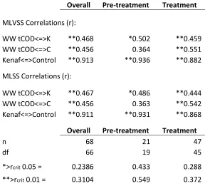
Table 3.2: Pearson Product-Moment Correlation Coefficients with 2-tailed critical values (rcrit)
Overall Pre-treatment Treatment MLVSS Correlations (r):
WW tCOD<=>K **0.468 *0.502 **0.459 WW tCOD<=>C **0.456 0.364 **0.551 Kenaf<=>Control **0.913 **0.936 **0.882 MLSS Correlations (r):
WW tCOD<=>K **0.467 *0.486 **0.444 WW tCOD<=>C **0.456 0.363 **0.542 Kenaf<=>Control **0.911 **0.931 **0.868 Overall Pre-treatment Treatment
n 68 21 47
df 66 19 45
*>rcrit 0.05 = 0.2386 0.433 0.288
**>rcrit 0.01 = 0.3104 0.549 0.372
45
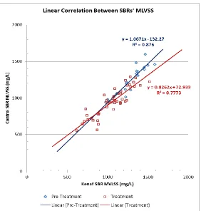
SBRs in their responses to environmental changes during Treatment than was evident in Pre-Treatment, in that the slope of the Treatment phase regression line was farther from the null hypothesis’s ideal value of 1. If the only difference between the reactors’ solids concentrations could be accounted for by the mass of kenaf added, the Treatment phase regression line would be expected to shift to the right of the Pre-Treatment phase regression line but still have a slope of approximately one.
46
47 Sludge Volume Index
The sludge volume index (SVI) was significantly improved by kenaf addition, as shown in Figure 3.8. Both reactors’ MLs had average SVIs near 190 mL/g before treatment. A paired sample 2-tailed T test of the reactors’ pre-treatment SVIs failed to refute the null hypothesis that the reactors were undifferentiated. While the average SVI of the control SBR’s ML did not change during the treatment phase, the kenaf supplemented ML’s average SVI dropped to about 130mL/g. As
detailed in Table 3.3, the treatment phase average SVIs of the reactors were significantly different at the alpha = 0.01 level, which supports the claim that kenaf supplementation leads to improved sludge settling. All kenaf application rates tested had similar effects on SVI, suggesting that the effect was not highly sensitive to the kenaf dose. Depending on plant design, improved sludge settling could reduce the volume of waste activated sludge (WAS) for processing or disposal, or return more biomass to the beginning of the treatment train allowing the plant to increase its organic loading rate.
Table 3.3: Summary of SVI statistics
Pre-Treatment Treatment
Kenaf ML
mean 192 mL/g 132 mL/g
S.D. 58.0 mL/g 16.55 mL/g
Control ML
mean 187 mL/g 190 mL/g
S.D. 44.6 mL/g 39.29 mL/g
n 18 46
T.test p(φ) = 0.4024 **6.0E-15
48
49 Heavy Metals
50
Table 3.4: Mean metals concentrations in 6 samples of dried sludge solids
SSolids Arsenic Cadmium Cobalt Chromium Copper Nickel Lead Selenium Zinc
mg/L μg/g μg/g μg/g μg/g μg/g μg/g μg/g μg/g μg/g
Kenaf ML
mean 1293 1.06 16.27 1.75 15.12 392.9 30.7 23.62 3.01 1429
S.D. 137 0.26 30.08 0.31 1.05 40.0 24.5 7.06 0.27 401
Control ML
mean 1232 0.75 19.81 1.99 16.01 267.8 35.7 11.84 3.45 1081
S.D. 149 0.30 46.11 0.40 1.96 37.9 41.2 7.45 0.30 303
t.TEST 0.169 **0.00913 0.653 *0.0343 0.121 **1.18E-05 0.597 **1.23E-04 **0.00808 *0.0324
51
Figure 3.9: Arsenic concentrations in dried sludge solids from kenaf supplemented and control SBRs.
52
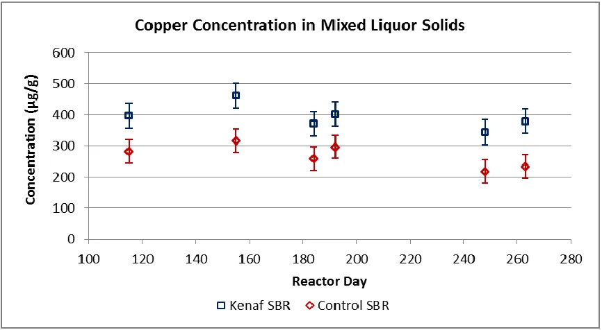
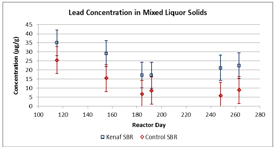
Figure 3.11: Lead concentrations in dried sludge solids from kenaf supplemented and control SBRs.
Increased zinc concentrations in the kenaf supplemented reactor were not apparent from Figure 3.12, and were not significant at the alpha = 0.01 level, but were significant at the alpha = 0.05 level.
Selenium was significantly (alpha = 0.01) less concentrated in the kenaf enriched sludge solids as shown in Figure 3.13. Cobalt (Figure 3.14) was also significantly (alpha = 0.05) less concentrated in the kenaf solids
53
Figure 3.12: Zinc concentrations in dried sludge solids from kenaf supplemented and control SBRs.
54
Figure 3.14: Cobalt concentrations in dried sludge solids from kenaf supplemented and control SBRs.
55
Figure 3.16: Chromium concentrations in dried sludge solids from kenaf supplemented and control SBRs.
56 Floc size
57
Figure 3.18: Fraction of total volume of particles having equivalent radii smaller than x μm on Dec. 31, 2011.
58
37.5% as many particles, the kenaf ML had a slightly larger (6%) total equivalent volume than control’s.
Figure 3.19: Fraction of total volume of particles having equivalent radii smaller than x μm on April
4, 2012.
Starting with the same raw particle size data used to generate the PSDs above, as well as that from 8 other pairs of samples, Figure 3.20 summarizes the distributions of particle sizes as their volume-moment means or D43s. For this plot, the Integrated Morphometry Analysis results from the 3
59
The mean D43s of the 3 petri dishes from each ML sample are shown in Figure 20 with error bars at
± one standard deviation. It is evident from Figure 3.20 that the kenaf floc tended to be larger, but also more variable in size than the control floc. A t Test comparing the 10 mean D43s from each
reactor rejected the null hypothesis at the alpha = 0.01 confidence level which provides evidence that there is a significant difference between the reactors in the distributions of floc sizes. This difference in floc size distributions could provide an explanatory mechanism for the observed improvements in the kenaf treated SBR’s Sludge Volume Index. It is also worth noting that the actual difference between the distributions is underestimated in this analysis in that this method was unable to image and analyze the largest kenaf particles.
Figure 3.20: Mean D43s for kenaf supplemented and control floc with error bars at ± one standard
60 Chemical Oxygen Demand
The control and kenaf supplemented reactors’ effluent concentrations of sCOD and tCOD did not diverge significantly in the course of this study, as illustrated by Figure 3.21. Summary statistics are given in Table 3.5, including results of paired sample 2-tailed t Tests comparing the reactors’ performances. Note that sCOD and tCOD values were not significantly different (alpha = 0.05) between the SBRs in the Pre-Treatment phase, nor were they in the Treatment phase.
61
Table 3.5: Summary of COD statistics
Pre-Treatment Treatment
Kenaf sCOD
Mean 29.6 mg/L 30.9 mg/L
S.D. 8.7 mg/L 6.2 mg/L
Control sCOD
Mean 28.3 mg/L 29.6 mg/L
S.D. 7.3 mg/L 4.7 mg/L
n 18 64
T.TEST(K<=>C) 0.0585 0.104
Kenaf tCOD
Mean 62.4 mg/L 52.3 mg/L
S.D. 26.2 mg/L 10.0 mg/L
Control tCOD
Mean 59.4 mg/L 49.7 mg/L
S.D. 23.5 mg/L 8.4 mg/L
n 18 65
T.TEST(K<=>C) 0.200 0.050
62
control reactors’ effluent sCOD or tCOD values were found to be significantly correlated (alpha = 0.01) to each other, as would be expected. In the Treatment phase the control effluent sCOD and tCOD continued to not correlate significantly with the influent strength. However, there was an unexpected significant (alpha = 0.05) correlation between influent strength and the kenaf SBR’s sCOD and tCOD.
63
Figure 3.23: Influent and effluent tCOD.
Table 3.6: Linear correlation coefficients
Pre-Treatment Treatment
sCOD
r(WW<=>K) 0.0544 0.293 *
r(WW<=>C) -0.0186 0.213
r(K<=>C) 0.9593 ** 0.303 *
n 18 64
*> rcrit 0.05 0.468 0.246
**> rcrit 0.01 0.590 0.320
tCOD
r(WW<=>K) -0.308 0.278 *
r(WW<=>C) -0.222 0.089
r(K<=>C) 0.930 ** 0.366 **
n 18 64
*> rcrit 0.05 0.468 0.246
64
In Figure 3.24 the data used to generate Figures 3.22 and 3.23 was plotted as percent removal of COD by each reactor. Percent removal of sCOD and tCOD was not found to differ significantly between the reactors during either the Treatment or Treatment phases of this study. In the Pre-Treatment phase both reactors had mean percent removal values near 71% for sCOD and 85% for tCOD. In the Treatment phase, both SBRs removed approximately 66% of sCOD and 87% of tCOD. Subsequent testing of aliquots of each ML, which had been subjected to extended saturation aeration, suggested that the fraction of sCOD or tCOD removed by the reactors was approximately equal to the biodegradable portion of the influent wastewater.
65 Nitrogen species
Effluent Total Nitrogen (TN) concentrations, both soluble and total, of the reactors are shown in Figure 3.25. Note that in the Pre-Treatment phase, TN concentrations varied considerably over time but were closely matched between the reactors at any given moment. During the Treatment phase there are periods of consistently low TN concentrations in which the SBRs seem to be performing similarly, interspersed with periods of extreme excursions from the typically low TN concentrations during which the control TN concentration increased more than the kenaf treated reactor’s did. Summary statistics in Table 3.7 suggest that there was not a significant difference (paired sample 2-tailed t Test, alpha = 0.01) between the SBRs’ performances in the Pre-Treatment phase. However the mean TN concentration of the control SBR’s effluent in the Treatment phase was approximately 2 mg/L higher than the kenaf treated SBR’s, which the two tailed t Test found to be a significant difference at the alpha = 0.01 confidence level.
66
Table 3.7: Effluent Total Nitrogen summary statistics
Pre-Treatment Treatment
Kenaf sTN
Mean 12.8 mg/L 5.7 mg/L
S.D. 6.5 mg/L 3.8 mg/L
Control sTN
Mean 11.7 mg/L 7.9 mg/L
S.D. 6.4 mg/L 7.3 mg/L
n 16 63
T.TEST(K<=>C) 0.1307 **0.0021 Kenaf tTN
Mean 15.7 mg/L 6.9 mg/L
S.D. 6.8 mg/L 3.6 mg/L
Control tTN
Mean 14.1 mg/L 8.9 mg/L
S.D. 5.7 mg/L 7.3 mg/L
n 16 62
T.TEST(K<=>C) *0.0193 **0.0056
67
Figure 3.26: Percent removal of Total Nitrogen.
Table 3.8: Percent removal of Total Nitrogen
Pre-Treatment Treatment
Kenaf sTN
Mean 71.5% 87.0%
S.D. 13.8% 7.8%
Control sTN
Mean 73.9% 82.3%
S.D. 13.4% 15.5%
n 16 63
T.TEST(K<=>C) *0.1048 **0.0029 Kenaf tTN
Mean 72.1% 87.3%
S.D. 11.4% 5.9%
Control tTN
Mean 74.9% 83.9%
S.D. 10.2% 11.9%
n 16 62
68
The Aeration Ratio (AR) was developed as an operational parameter to aid in standardizing the aeration intensity to the varying influent strength, but it can also help explain the variability in nitrogen removal performance, as illustrated by Figure 3.27 in which the sTN removal performance can be observed to de-optimize whenever the AR drops below a value of approximately 11. The Aeration Ratio is the mass of oxygen supplied to the mixed liquor by the aeration pump divided by the mass of oxygen utilized by the reactor (i.e. influent tCOD load – effluent tCOD load, or tCOD exerted), and therefore can be considered a unitless value. AR is a function of both the wastewater feedstock’s tCOD and of the airflow in liters per minute during the aerobic portions of the treatment cycle.
The AR does not attempt to estimate the amount of oxygen that transfers from the aeration bubbles to the bulk liquid. The typical ambient temperature of the lab (23°C) was used for all AR
69
The AR was very useful for operating the reactors, but this ratio can also provide a way to quantify the degree of departure from optimal growth conditions in the SBRs in order to evaluate the impact those departures have on plant performance. Unfortunately, the airflow regulators used for this study demonstrated a tendency to wander from their intended settings. The airflow values
recorded were those observed after the reactors had run unattended for several cycles. Because of the instability of the regulators, the SBRs’ airflow readings did not always match each other. A 3 day running average of AR values reduced the effect of brief excursions from the intended airflow.
70
In order to compare the behavior of the SBRs under optimal and non-optimal conditions, two blocks of data were extracted from the main dataset. One block consisted of AR values and TN
concentrations from Treatment phase days on which both reactors were observed to have ARs greater than 11. In the other block, both systems had ARs of less than 11. In the high AR block, the mean AR for both SBRs was 14.3, the mean sTN values were 4.8 mg/L for kenaf and 4.9 mg/L for control and mean tTN concentrations were 6.3 mg/L for kenaf and 6.2 mg/L for control. Both systems removed approximately 88% of sTN and tTN. No significant differences between the plants were detected in this block. By contrast, in the low AR block both reactors had mean ARs of 9.4. The kenaf supplemented SBR’s effluent had an average of 7.0 mg sTN/L and 8.5 mg tTN/L, but the control’s effluent averaged 10.5 mg sTN/L and 11.8 mg tTN/L, a significant difference at the alpha = 0.01 confidence level. Removal performance was also significantly different (alpha = 0.01) in this block, with control removing approximately 78% of sTN and tTN, while the kenaf SBR was able to remove an average of 85% of sTN and tTN. This suggests that when aeration is below the optimal intensity, as might happen in a full scale plant when a bolus of unusually high COD waste enters the treatment train, nitrogen removal performance of the kenaf supplemented mixed liquor is not as adversely affected as that of untreated ML.
71
though this analysis maintained soluble and total concentrations as distinct data sets. For clarity, only the results from filtered samples are shown in Figure 3.28. As detailed in Table 3.9, during the Pre-Treatment stage mean sNH3-N concentrations were 3.8 mg/L for the kenaf reactor and 4.7 mg/L for control which was not a significant difference at the alpha = 0.05 confidence level. Mean tNH3-N was 4.0 mg/L for the kenaf SBR and 5.5 mg/L for control which was not a significant difference at the alpha = 0.01 level. In the Treatment stage mean sNH3-N for the kenaf reactor was 2.7 mg/L while control’s was significantly different (alpha = 0.01) at 5.3 mg/L. Mean tNH3-N values were 3.0 mg/L for the kenaf supplemented SBR and 5.8 mg/L for the control, which is a significant difference at the alpha = 0.01 confidence level. Much like Total Nitrogen, the Treatment phase was marked by periods of very low effluent ammonia-nitrogen in both reactors alternating with periods of instability in which the control’s effluent NH3-N peaked at a much higher value than the kenaf supplemented SBR’s effluent concentration.
72
Table 3.9: Effluent ammonia-nitrogen concentrations
Pre-Treatment Treatment
Kenaf sNH3-N
Mean 3.8 mg/L 2.7 mg/L
S.D. 5.9 mg/L 4.1 mg/L
Control sNH3-N
Mean 4.7 mg/L 5.3 mg/L
S.D. 6.9 mg/L 7.6 mg/L
n 15 61
T.TEST(K<=>C) 0.0817 0.0002
Kenaf tNH3-N
Mean 4.0 mg/L 3.0 mg/L
S.D. 6.3 mg/L 4.3 mg/L
Control tNH3-N
Mean 5.5 mg/L 5.8 mg/L
S.D. 7.9 mg/L 7.6 mg/L
n 15 66
T.TEST(K<=>C) 0.0286 2.22E-05
Converting the data from Figure 3.28 to ammonia-nitrogen removal rates removes the influent variability as a source of the peaks in effluent concentration. However, the periods of poor performance were still evident as can be seen in Figure 3.29. During the Pre-Treatment stage the kenaf reactor removed 89% of sNH3-N, and control removed 86%. The control SBR removed 86% of tNH3-N while the reactor designated for subsequent kenaf treatment removed 90%. Neither
73
control continued to remove 86%. The kenaf reactor removed 92% of tNH3-N to control’s 85%. As shown in Table 3.10, the differences between the reactors’ NH3-N removal performances during treatment were significant at the alpha = 0.01 confidence level.
74
Table 3.10: Percent of ammonia-nitrogen removed by kenaf and control SBRs
Pre-Treatment Treatment
Kenaf %Rmvl sNH3-N
Mean 88.7% 93.2%
S.D. 17.8% 10.3%
Control %Rmvl sNH3-N
Mean 86.0% 86.3%
S.D. 20.8% 19.3%
n 15 61
T.TEST(K<=>C) 0.0809 0.0002
Kenaf %Rmvl tNH3-N
Mean 90.1% 92.2%
S.D. 15.7% 10.9%
Control %Rmvl tNH3-N
Mean 86.2% 84.6%
S.D. 19.4% 19.6%
n 15 66
T.TEST(K<=>C) 0.0260 2.02E-05
75
sNH3-N leaving 4.8 mg/L sNH3-N in its effluent. On the other hand, the control reactor removed only 78% of sNH3-N leaving mean effluent concentrations of 8.6 mg/L sNH3-N. The differences between the systems’ performances in the low AR block were significant at the 0.01 confidence level. This suggests that, as with Total Nitrogen, when aeration is below the optimal intensity, ammonia-nitrogen removal performance of the kenaf supplemented mixed liquor is not as adversely affected as that of untreated ML.
Effluent nitrite-nitrogen and nitrate-nitrogen concentrations are plotted in Figure 3.30 along with the 3 day running average Aeration Ratio. Nitrate was only detected in significant amounts during the startup Pre-Treatment stage. However, small amounts of NO2-N (less than 5 mg N/L) were
common in the effluent whenever the AR was above a value of approximately 10. Nitrite-nitrogen concentrations were strongly positively correlated (alpha= 0.01) with the 3 day running average AR. The mean nitrite-nitrogen concentrations in the kenaf and control SBRs in the Pre-Treatment phase were 2.0 mg/L and 1.7 mg/L respectively, which was not a significant difference at the alpha = 0.05 confidence level according to the paired sample 2-tailed t Test. During the Treatment phase, the kenaf treated reactor’s mean NO2-N was 1.6 mg/L to control’s 1.1 mg/L. This difference was
significant at the alpha = 0.01 confidence level. Because the reactors ran a nit-denit treatment cycle it is unclear whether this result represents more efficient oxidation of ammonia to nitrite or less effective de-nitrification by the kenaf supplemented mixed liquor. Removal rates for
76
77 Total Phosphate
The percent of Total Phosphate removed by each reactor is plotted in Figure 3.31 along with the 3 day running average Aeration Ratio. Optimum phosphate removal appears to occur when the AR is between 8 and 10. Too much aeration led to reduced phosphate removal, probably because residual dissolved oxygen persisted for too long into what would otherwise be the anaerobic selector phase. Too little aeration failed to provide aerobic conditions for growth of Phosphate Accumulating Organisms, which also caused a decrease in phosphate removal. No significant differences in the reactors’ performances were detected in either the Pre-Treatment or the Treatment phases.
78 Intra-Cycle Samples
Intensive sampling within a single treatment cycle of each reactor’s mixed liquor made it possible to track internal changes in the concentration of soluble COD and soluble nitrogen species. Only soluble species were measured because results from unfiltered ML samples would not have been comparable to those generated by this study from unfiltered effluent. A subsequent cycle at the same time the next day was similarly sampled and yielded results nearly identical to those presented here.
Figure 3.32 shows the soluble COD concentrations within the reactors through one 4 hour cycle. Note that the resolution of the sCOD test used was ±2 mg/L, which is not ideal for discerning changes within a range of just over 10 mg/L. A paired sample 2-tailed t Test found no significant differences between the reactors’ sCOD concentrations.
79
Variations in the concentration of soluble Total Nitrogen through one cycle are plotted in Figure 3.33. A paired sample 2-tailed t Test found that the differences in reactor sTN concentration were significant. However, the magnitude of those differences was less than 2 mg/L. The reported resolution of the Hach TN test is ±0.5 mg/L.
Figure 3.33: Soluble Total Nitrogen in ML through one SBR treatment cycle.
80
question the significance of this result. It is worth noting that measurements of standard solutions in our lab were generally within 1 mg/L of the analytically derived concentration.
Figure 3.34: Soluble ammonia-nitrogen in ML through one SBR treatment cycle.
81
Figure 3.35: Nitrite-nitrogen in ML through one SBR treatment cycle.
Figure 3.36 shows a significant difference (alpha = 0.01) between the reactors in their nitrate-nitrogen concentrations, with the kenaf supplemented SBR’s NO3-N peaking at a level over twice as