University of Windsor University of Windsor
Scholarship at UWindsor
Scholarship at UWindsor
Electronic Theses and Dissertations Theses, Dissertations, and Major Papers
2012
A structural investigation to develop guidelines for the finite
A structural investigation to develop guidelines for the finite
element analysis of the Mini-Baja vehicle
element analysis of the Mini-Baja vehicle
Babak Shahabi University of Windsor
Follow this and additional works at: https://scholar.uwindsor.ca/etd
Recommended Citation Recommended Citation
Shahabi, Babak, "A structural investigation to develop guidelines for the finite element analysis of the Mini-Baja vehicle" (2012). Electronic Theses and Dissertations. 5342.
https://scholar.uwindsor.ca/etd/5342
This online database contains the full-text of PhD dissertations and Masters’ theses of University of Windsor students from 1954 forward. These documents are made available for personal study and research purposes only, in accordance with the Canadian Copyright Act and the Creative Commons license—CC BY-NC-ND (Attribution, Non-Commercial, No Derivative Works). Under this license, works must always be attributed to the copyright holder (original author), cannot be used for any commercial purposes, and may not be altered. Any other use would require the permission of the copyright holder. Students may inquire about withdrawing their dissertation and/or thesis from this database. For additional inquiries, please contact the repository administrator via email
A STRUCTURAL INVESTIGATION TO DEVELOP GUIDELINES
FOR THE FINITE ELEMENT ANALYSIS OF THE MINI-BAJA
VEHICLE
By
Babak Shahabi
A Thesis
Submitted to the Faculty of Graduate Studies
through the Department of Mechanical, Automotive and Materials Engineering in Partial Fulfillment of the Requirements for
the Degree of Master of Applied Science at the University of Windsor
Windsor, Ontario, Canada
2011
A structural investigation to develop guidelines for the finite element analysis of the Mini-Baja vehicle
by
Babak Shahabi
APPROVED BY:
______________________________________________ Dr. S. Das (Outside Program Reader)
Department of Civil & Environmental Engineering
_____________________________________________ Dr. R. Barron (Program Reader)
Department of Mechanical, Automotive and Materials Engineering
______________________________________________ Dr. N. Zamani (Advisor)
Department of Mechanical, Automotive and Materials Engineering
______________________________________________ Dr. S. Erfani (Co-advisor)
Department of Electrical & Computer Engineering
______________________________________________ Dr. B. Zhou (Chair of Defence)
Department of Mechanical, Automotive and Materials Engineering
III
AUTHOR’S DECLARATION OF ORIGINALITY
I hereby certify that I am the sole author of this thesis and that no part of this thesis has been published or submitted for publication.
I certify that, to the best of my knowledge, my thesis does not infringe upon anyone‟s
copyright nor violate any proprietary rights and that any ideas, techniques, quotations, or any other material from the work of other people included in my thesis, published or
otherwise, are fully acknowledged in accordance with the standard referencing practices. Furthermore, to the extent that I have included copyrighted material that surpasses the bounds of fair dealing within the meaning of the Canada Copyright Act, I certify that I have obtained a written permission from the copyright owner(s) to include such material(s) in my thesis and have included copies of such copyright clearances to my appendix.
IV
ABSTRACT
Mini-Baja is a special type of vehicle used for recreational and exploration purposes. In many aspects it is similar to an All-Terrain Vehicle (ATV) except that it is much smaller in size. An international competition is organized by the Society of Automotive Engineers (SAE) for universities throughout the world to design and fabricate their vehicles and then compete against each other.
The objective of the present research was to carry out finite element analysis and crash simulations for a Mini-Baja chassis structure. The aim of this task was to write a comprehensive finite element guide for a Mini-Baja SAE vehicle that had already been built by students at the University of Windsor for the year 2010 Baja competition in Rochester New York.
Initially, an example of a Z-frame is explained and evaluated by simple hand calculations. Subsequently, the preliminary design of the Mini-Baja roll cage was generated using CAD data. To study the effects of stress and deformation on the frame members, linear static analysis followed by transient modal superposition analysis was carried out as the first steps toward this project. The static analysis in this thesis was used to arrive at an acceptable mesh size for the Mini-Baja roll cage dynamic analysis.
Additionally, the more realistic frontal impact analysis was performed on the Mini-Baja vehicle at a cruise velocity of 48 km/h (30 mph). Different FEA commercial
packages were used throughout the project and results obtained from Abaqus/CAE and LS-DYNA were compared with one another.
V
DEDICATION
Dedicated to my parents and my brother,
VI
ACKNOWLEDGEMENTS
I would like to express my most sincere gratitude and profound appreciation to Dr. Nader Zamani for his supervision, guidance and support. His knowledge and expertise has been of immeasurable assistance throughout my graduate studies and research. This work could not have been achieved without his help and support.
I owe my deepest gratitude to Dr. William Altenhof for his guidance and encouragement. I appreciate all his contributions to make my experience productive and stimulating at the University of Windsor. The joy and enthusiasm he has for his research was contagious and motivational for me throughout my graduate degree.
I would like to take this opportunity to also thank my co-advisor Dr. S. Erfani, and my committee members Dr. S. Das and Dr. R. Barron for helping me throughout this thesis.
Lastly, I offer my regards and blessings to my friends, colleagues, and all of those who supported me in any respect during the completion of this thesis.
VII
TABLE OF CONTENTS
AUTHOR’S DECLARATION OF ORIGINALITY --- III
ABSTRACT --- IV
DEDICATION --- V
ACKNOWLEDGEMENTS --- VI
LIST OF TABLES --- XI
LIST OF FIGURES --- XII
LIST OF APPENDICES --- XXI
NOMENCLATURE --- XXII
CHAPTER І --- 1
1. INTRODUCTION --- 1
1.1 Scope and objective of the project --- 1
1.2 About the SAE Mini-Baja --- 2
1.3 The CAD model of the Mini-Baja frame and chassis --- 3
1.4 The role of non-linearities in the analysis of Mini-Baja--- 7
1.5 Literature review --- 12
1.5.1 Literature review of “SAE Mini-Baja” capstone reports --- 12
1.5.2 Literature review of “Vehicle Crash Impact Analysis” papers --- 23
CHAPTER ІІ --- 37
2. FINITE ELEMENT THEORY WITH NUMERICAL EXAMPLE --- 37
2.1 Objectives and overview of Chapter ІІ --- 37
VIII
2.3 Finite element analysis fundamentals --- 38
2.4 Finite element form of the assumed solution --- 39
2.5 Finite element library --- 42
2.6 Z-frame example --- 43
2.6.1 Computer implementation (Matlab) for the Z-frame --- 47
2.6.2 Computer simulation (Catia) for the Z-frame --- 52
2.6.3 Z-frame modified --- 54
CHAPTER ІІІ --- 61
3. APPLICATION OF BEAM, SHELL, AND SOLID ELEMENTS FOR THE MINI-BAJA FRAME (LINEAR STATIC AND DYNAMIC ANALYSIS) --- 61
3.1 Objectives and overview of Chapter ІІІ --- 61
3.2 Mini-Baja modeling methodology --- 61
3.2.1 Material properties --- 65
3.2.2 Section property --- 68
3.2.3 Loading condition--- 68
3.2.4 Connections --- 70
3.3 Static results --- 71
3.4 Transient dynamic analysis --- 76
3.4.1 Damping effect --- 78
3.4.2 Dynamic force --- 79
3.4.3 Transient dynamic simulation --- 80
3.5 Mesh convergence study --- 87
CHAPTER ІV --- 92
4. NON-LINEAR DYNAMIC ANALYSIS OF THE MINI-BAJA FRAME IN FRONTAL CRASH (LS-DYNA) --- 92
4.1 Objectives and overview of Chapter ІV --- 92
4.2 Key parameters of a non-linear explicit vehicle simulation --- 93
4.2.1 Implicit vs. explicit time integration methodologies --- 93
4.2.2 Viscoplastic material model --- 95
IX
4.2.4 Hourglass energy modes --- 101
4.2.5 Time step and mass scaling --- 102
4.2.6 Contact and friction modeling --- 103
4.3 Simulation of the front portion of the frame (LS-DYNA) --- 107
4.4 Frontal impact simulation of the Mini-Baja frame structure (LS-DYNA) --- 112
4.4.1 Energy balance --- 118
CHAPTER V --- 121
5. EVALUATION OF THE FRONTAL CRASH OF THE MINI-BAJA VEHICLE BY (ABAQUS/CAE) --- 121
5.1 Objectives and overview of Chapter V --- 121
5.2 Simulation of the front portion of the frame (Abaqus/CAE) --- 122
5.3 Frontal impact simulation of the Mini-Baja frame chassis (Abaqus/CAE)--- 130
5.4 Further comparison of LS-DYNA and Abaqus/CAE results --- 134
CHAPTER VІ --- 139
6. A MORE COMPLETE MODEL OF THE MINI-BAJA VEHICLE FOR CRASH ANALYSIS (LS-DYNA) --- 139
6.1 Objectives and overview of Chapter VІ --- 139
6.2 Modeling of the tires --- 139
6.3 Simulation of the complete Mini-Baja vehicle --- 143
6.3.1 The frontal crash of the Mini-Baja vehicle --- 147
6.3.2 The side crash of the Mini-Baja vehicle --- 153
6.3.3 Head-on collision of two Mini-Baja vehicles at 30 degree impact angle --- 157
CHAPTER VІІ --- 161
7. CONCLUSIONS AND RECOMMENDATIONS FOR FUTURE WORK --- 161
7.1 Conclusions --- 161
7.2 Recommendations for future work --- 163
X
APPENDICES --- 171
APPENDIX A --- 172
A. SEAM WELD CONNECTION --- 172
APPENDIX B --- 173
B. WIREFRAME LINE CONNECTION ISSUE --- 173
APPENDIX C --- 174
C. TRANSIENT DYNAMIC ANALYSIS --- 174
XI
LIST OF TABLES
Table 2.1 Nodal displacement of the Z-frame --- 54
Table 2.2 Nodal rotations of the Z-frame --- 54
Table 2.3 Frequency analysis of the Z-frame ( , --- 57
Table 2.4 von Mises stress for Z-frame ( , --- 60
Table 3.1 Alloy composition of 4130 chromoly (by weight) [35] --- 66
Table 3.2 Mechanical properties of 4130 steel [35] --- 66
Table 3.3 Structural property of 4130 chromoly used in static simulation --- 67
Table 3.4 Number of modes and corresponding natural frequencies --- 82
Table 3.5 Variation of maximum displacement and stress due to change in shell element size -- 87
Table 3.6 Displacement and stress at selected points in the frame --- 90
Table 4.1 Effect of different hourglass control techniques on accuracy and computational time ---108
Table 4.2 Effect of adaptive method on zero energy modes --- 109
XII
LIST OF FIGURES
Figure 1.1 University of Windsor Mini-Baja vehicle, 2010 --- 2
Figure 1.2 University of Windsor Mini-Baja vehicle, 2010 --- 3
Figure 1.3 Preliminary design of the chassis from SAE rule guide [1] --- 5
Figure 1.4 Preliminary design of the chassis from SAE rule guide [1] --- 5
Figure 1.5 CAD model of the Mini-Baja vehicle --- 6
Figure 1.6 CAD model of the Mini-Baja chassis --- 6
Figure 1.7 Behaviour of transverse beam sections in (a) slender beams and (b) thick beams [8] -- 9
Figure 1.8 Large deflection of a cantilever beam [8] --- 9
Figure 1.9 Non-linear load-displacement curve [8] --- 10
Figure 1.10 Front impact – loading point of application [14] --- 13
Figure 1.11 Full meshed model in Ansys [15] --- 14
Figure 1.12 Front impact scenario in Visual Nastran [16] --- 18
Figure 1.13 Rollover impact scenario in Visual Nastran [16] --- 19
Figure 1.14 Left: finite element mesh with masses and rigid-walls; Right: optimized design of the chassis [17] --- 21
Figure 1.15 Deformation of the chassis at 0.030 sec [17] --- 22
Figure 1.16 Energy plot for frontal impact [17] --- 22
Figure 1.17 The chassis frame [18] --- 23
Figure 1.18 Idealization with 58 and 22 nodes [18] --- 24
XIII
Figure 1.20 Flow chart of the project with digitization [20] --- 27
Figure 1.21 Consumer information label for a vehicle with at least one NCAP star rating [22] -- 28
Figure 1.22 Crush depth location and comparison [21] --- 29
Figure 1.23 Crash output results at different stages of the simulation [21] --- 30
Figure 1.24 FE model of the 2006 Ford F250 [23] --- 31
Figure 1.25 Left: comparison of the global deformation for NCAP test and simulation; Right: simulation data for energy balance [23] --- 32
Figure 1.26 Simulation and impact test comparison [25] --- 33
Figure 1.27 Finite element model of the C2500 pickup truck [26] --- 34
Figure 1.28 Comparison of pendulum test 02025 and simulation [26] --- 35
Figure 1.29 Comparison of pendulum test 02027 and simulation [26] --- 35
Figure 2.1 Element generation --- 40
Figure 2.2 Beam element with uniform cross-section --- 41
Figure 2.3 Element library of LS-DYNA [30] --- 42
Figure 2.4 Z-frame setup --- 44
Figure 2.5 An arbitrary oriented frame element --- 45
Figure 2.6 Three-element model for the Z-frame --- 46
Figure 2.7 FE model of the Z-frame --- 52
Figure 2.8 Nodal displacement of the Z-frame --- 53
Figure 2.9 FE model of the Z-frame with beam, shell and solid elements --- 56
XIV
Figure 2.11 Vertical vibration behaviour of beam, shell and solid models --- 58
Figure 2.12 Horizontal vibration behaviour of beam, shell and solid models --- 59
Figure 2.13 Out of plane mode of vibration of beam, shell and solid models --- 59
Figure 2.14 von-Mises stress contour; shell and solid --- 60
Figure 3.1 Linear tetrahedron solid element [34] --- 62
Figure 3.2 Solid idealization of the Mini-Baja structure --- 63
Figure 3.3 Linear triangular shell element [34] --- 64
Figure 3.4 Shell idealization of the Mini-Baja structure --- 64
Figure 3.5 Beam idealization of the Mini-Baja structure --- 65
Figure 3.6 Stress-strain curves of different grades of steel [35] --- 67
Figure 3.7 Sectional property of beam and shell models --- 68
Figure 3.8 Linear impulse and momentum applied on Mini-Baja frontal collision --- 69
Figure 3.9 Seam welded connection CATIA V5 --- 70
Figure 3.10 Weld-connection for the beam model CATIA V5 --- 71
Figure 3.11 Deformation shape for the beam model --- 72
Figure 3.12 Deformation shape for the shell model --- 73
Figure 3.13 Deformation shape for the solid model --- 74
Figure 3.14 von Mises stress distribution for the shell model --- 75
Figure 3.15 von Mises stress distribution for the solid model --- 75
XV
Figure 3.17 Structure response for different types of damping [37] --- 78
Figure 3.18 Schematic diagram of a vehicle model over a bump --- 79
Figure 3.19 Constraint condition for dynamic analysis --- 80
Figure 3.20 Constraint condition for dynamic analysis --- 81
Figure 3.21 Deformation shape in static analysis --- 81
Figure 3.22 Stress contours in static analysis --- 82
Figure 3.23 Time modulation of the dynamic applied load --- 83
Figure 3.24 Maximum displacement of the frame at 0.0135 sec in dynamic analysis --- 84
Figure 3.25 Node for displacement graphs --- 84
Figure 3.26 Three components of the displacement response of the selected point for the time duration of 0.9 sec --- 85
Figure 3.27 Three components of the velocity response of the selected point for the time duration of 0.9 sec --- 85
Figure 3.28 Distribution of von Mises stress through the cage in time --- 86
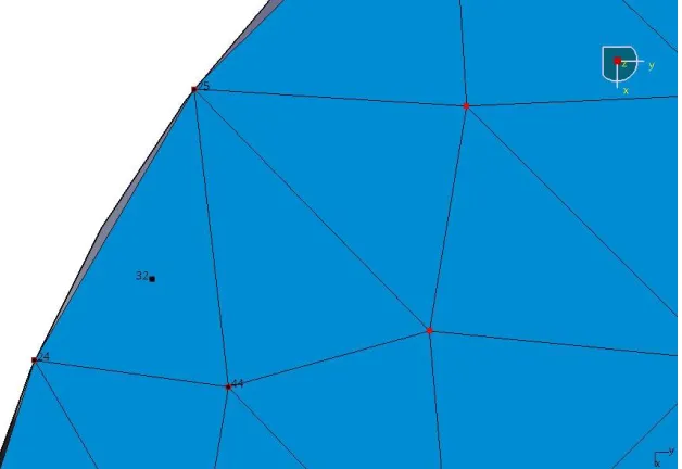
Figure 3.29 Mesh convergence study for maximum displacement --- 88
Figure 3.30 Mesh convergence study for maximum stress --- 88
Figure 3.31 Selection of points for the mesh convergence study --- 89
Figure 3.32 Mesh convergence study for displacement at selected points --- 90
Figure 3.33 Mesh convergence study for stress at selected points --- 91
Figure 4.1 Cost versus model size in explicit and implicit methodologies [8] --- 94
Figure 4.2 Determination of effective plastic strain --- 95
XVI
Figure 4.4 Stress-strain response of a viscoplastic material at different strain rates [39] --- 97
Figure 4.5 Yield stress vs. effective plastic strain at different strain rates [30] --- 98
Figure 4.6 A representation of membrane forces on a membrane element and bending moments on a plate element [40] --- 99
Figure 4.7 LS-DYNA shell elements, node numbering for normal direction [30] --- 99
Figure 4.8 Representation of warped shell elements [42] --- 100
Figure 4.9 a) A fully integrated element to the left and a under integrated element to the right; b) Two hourglass modes for the under integrated element [41] --- 101
Figure 4.10 Penalty contact algorithm in LS-DYNA [37] --- 104
Figure 4.11 Tied contact between tubes --- 105
Figure 4.12 Front portion of the vehicle --- 107
Figure 4.13 von Mises stress at different speeds for the front portion of the vehicle --- 107
Figure 4.14 Adaptive method applied on the frame --- 108
Figure 4.15 Hourglass energy vs. hourglass control models --- 109
Figure 4.16 Deformation shape of models with different adaptive refinements (in terms of the threshold angle) --- 110
Figure 4.17 Deformation vector of 4 different models --- 111
Figure 4.18 Energy balance for front portion at 150 km/h (model 1) --- 111
Figure 4.19 Mini-Baja frame structure --- 112
Figure 4.20 von Mises stress at 0.013 sec --- 113
Figure 4.21 Maximum von Mises stress at 0.015 sec --- 113
XVII
Figure 4.23 Strain rate of 0.08/s at 0.006 sec --- 114
Figure 4.24 Strain rate of 80/s at 0.0109 sec --- 115
Figure 4.25 Highest Strain rate of 132/s at 0.014 sec --- 115
Figure 4.26 Strain rate of 5/s at 0.038 sec --- 115
Figure 4.27 Velocity contour in y-direction at 0.0109 sec--- 116
Figure 4.28 Selected joints for contact force --- 116
Figure 4.29 Highest contact forces at the joints --- 117
Figure 4.30 Rigid wall normal force --- 117
Figure 4.31 Percentage of mass increase --- 118
Figure 4.32 Energy balance for the complete mock-up at 48 km/h --- 120
Figure 4.33 Energy ratio of the simulation at 48 km/h --- 120
Figure 5.1 Front portion of the frame in frontal impact setup (Abaqus/CAE) --- 122
Figure 5.2 Tie contact (Abaqus/CAE) --- 123
Figure 5.3 Energy balance for front portion at 60 km/h (Abaqus/CAE) --- 124
Figure 5.4 Energy balance for front portion at 60 km/h modified (Abaqus/CAE)--- 125
Figure 5.5 Energy balance for front portion at 60 km/h (LS-DYNA) --- 125
Figure 5.6 The ratio of artificial strain energy over elastic strain energy --- 126
Figure 5.7 von Mises stress distribution of the front portion at 60 km/h (LS-DYNA) --- 127
Figure 5.8 von Mises stress distribution of the front portion at 60 km/h (Abaqus/CAE) --- 127
Figure 5.9 von Mises stress distribution of the front portion at 150 km/h (Abaqus/CAE) --- 128
XVIII
Figure 5.11 Comparison of energy balance of the front portion at 150 km/h --- 129
Figure 5.12 Frontal impact scenario of the Mini-Baja vehicle (Abaqus/CAE) --- 130
Figure 5.13 Example of a wrong material direction --- 131
Figure 5.14 Energy balance of the frontal impact at 48 km/h (Abaqus/CAE) --- 132
Figure 5.15 von Mises stress distribution at 0.013 sec (Abaqus/CAE) --- 132
Figure 5.16 Maximum von Mises stress at 0.016 sec (Abaqus/CAE) --- 133
Figure 5.17 Maximum plastic strain at the end of the simulation 0.045 sec (Abaqus/CAE) --- 133
Figure 5.18 Maximum plastic strain at the end of the simulation 0.045 sec --- 134
Figure 5.19 Energy balance of the full Mini-Baja mock-up at 48 km/h --- 135
Figure 5.20 Selected point for side displacement --- 135
Figure 5.21 Side displacement of point (P) --- 136
Figure 5.22 Selected roof point (Q) --- 136
Figure 5.23 Vertical displacement of the roof point (Q) --- 137
Figure 5.24 Wall reaction force --- 138
Figure 5.25 Reaction wall force versus resultant displacement (stiffness) --- 138
Figure 6.1 Actual tires and suspension assembly --- 140
Figure 6.2 CAD model of the tire --- 140
Figure 6.3 FE model of the tire assembly displaying the sectional thicknesses --- 141
Figure 6.4 Deformation of the tires at 90mm displacement of the wall--- 142
XIX
Figure 6.6 FE model of the completed Mini-Baja vehicle --- 143
Figure 6.7 Body panels and nodal rigid body constrained --- 144
Figure 6.8 Body panels, rear suspension, and shocks --- 145
Figure 6.9 Behaviour of the low density foam [30] --- 145
Figure 6.10 Stress-strain curve for the low density foam cushion --- 146
Figure 6.11 Revolute joint and angular velocity of the tires --- 146
Figure 6.12 Test setup for equilibrium check --- 148
Figure 6.13 Reaction force of the rigid ground --- 148
Figure 6.14 Isometric view of the detailed model simulation of the Mini-Baja vehicle into the rigid wall at 48 km/h --- 149
Figure 6.15 Left: the maximum von Mises stress at 0.011 sec; Right: effective plastic strain at the end of the simulation --- 149
Figure 6.16 Side, top and front views of the deformation at t = 0.014 sec --- 150
Figure 6.17 Side, top and front views of the deformation at t = 0.025 sec --- 150
Figure 6.18 Side, top and front views of the deformation at t = 0.036 sec --- 150
Figure 6.19 Traced nodes on the rear tire at t = 0.04 sec --- 151
Figure 6.20 Energy balance for frontal crash at 48 km/h --- 151
Figure 6.21 Energy balance for frontal crash at 48 km/h (low density tire)--- 152
Figure 6.22 Kinetic energy based on density of tires at 48 km/h --- 152
Figure 6.23 Side impact setup --- 153
Figure 6.24 Sequential views of the side impact scenario 1 at initial position --- 154
XX
Figure 6.26 Sequential views of the side impact scenario 1 at the end of the simulation --- 154
Figure 6.27 Energy balance of the side crash scenario 1 at 48 km/h --- 155
Figure 6.28 Sequential views of the side impact scenario 2 at initial position --- 155
Figure 6.29 Sequential views of the side impact scenario 2 at t = 0.016 sec--- 156
Figure 6.30 Sequential views of the side impact scenario 2 at t = 0.025 sec--- 156
Figure 6.31 Sequential views of the side impact scenario 2 at the end of the simulation --- 156
Figure 6.32 Energy balance of the side crash scenario 2 at 48 km/h --- 157
Figure 6.33 Configuration of the vehicle-to-vehicle crash at 30 degree impact angle --- 158
Figure 6.34 Sequential views of the vehicle-to-vehicle crash at initial position --- 158
Figure 6.35 Sequential views of the vehicle-to-vehicle crash at t = 0.017 sec --- 159
Figure 6.36 Sequential views of the vehicle-to-vehicle crash at t = 0.036 sec --- 159
Figure 6.37 Sequential views of the vehicle-to-vehicle crash at t = 0.07 sec --- 159
Figure 6.38 Energy balance of the vehicle-to-vehicle crash at 48 km/h --- 160
Figure 6.39 Maximum von Mises stress for vehicle-to-vehicle crash at t = 0.02 sec --- 160
Figure 7.1 Hybrid III occupant dummy --- 164
Figure 7.2 Two Mini-Baja‟s impact scenario at 30 degree impact angle --- 165
Figure A.1 Seam weld connection tutorial --- 172
Figure B.1 Line connection issue tutorial --- 173
XXI
LIST OF APPENDICES
APPENDICES --- 171
APPENDIX A --- 172
A. SEAM WELD CONNECTION --- 172
APPENDIX B --- 173
B. WIREFRAME LINE CONNECTION ISSUE --- 173
APPENDIX C --- 174
XXII
NOMENCLATURE
Transverse shear strains
Linear stiffness matrix
Incremental matrix
Initial stress matrix
Degree of freedom
Stiffness matrix
Mass matrix
Damping matrix
Natural frequency of harmonic motion
Shape function
Distributed loads
Point loads and moments Plastic strain
Elastic strain
Strain rate
Initial yield stress
Static stress
Membrane forces
Characteristic length
c Sound speed
Bulk modulus
1
CHAPTER І
1. INTRODUCTION
1.1 Scope and objective of the project
In this thesis, considerable effort has been dedicated to the use of different commercial finite element analysis packages available at the University of Windsor. The intended objective of this thesis is to present some of the findings and challenges with regard of the finite element modeling of a Mini-Baja vehicle. It is anticipated that this research will assist undergraduate and graduate students or other readers who have limited experience in computational methods in using FEA tools for design purposes.
An introduction to the Mini-Baja vehicle, basic fundamentals of simulation, and the assumptions made for the non-linear dynamic analysis of the vehicle are discussed in Chapter 1. The finite element method and its application for a simple Z-frame is discussed in Chapter 2. There, the numerical results of a linear finite element analysis are compared with theoretical solution using a Matlab program.
In Chapter 3, the application of shell, beam and solid elements for a Mini-Baja frame are discussed for a linear static analysis. Later in this chapter, dynamic loads transmitted to the frame are simulated for a case where the vehicle goes over a bump. Chapter 4 provides an explicit non-linear dynamic simulation for a frontal crash of the frame into a rigid wall at 48 km/h (30mph). The results from this simulation are validated by another FEA package in Chapter 5.
2
1.2 About the SAE Mini-Baja
The Society of Automotive Engineers (SAE) organizes an inter-collegiate competition in which various universities from all around the world build a Mini-Baja
vehicle to compete against one another. The automotive society has laid down a set of guidelines and rules [1] that every vehicle should follow. These guidelines are based on recommendations and tests conducted by design professionals and engineers.
Being a competition, every university has to develop its own design without any professional assistance or knowledge sharing. Baja SAE consists of three regional competitions that simulate real-world engineering design projects and their related challenges. Engineering students are tasked to design and build an off-road vehicle that will survive the severity of rough terrain and sometimes even water.
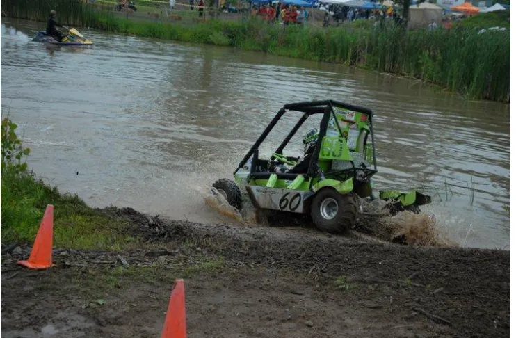
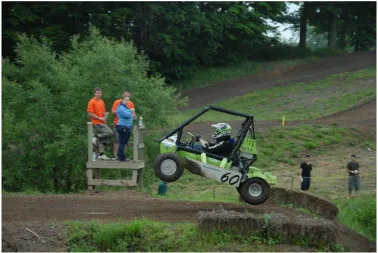
Figure 1.1 University of Windsor Mini-Baja vehicle, 2010
3
The mechanical engineering capstone project is an attempt to design a Mini-Baja from scratch, based on the guidelines provided by SAE. Certain practices by the industry in off-road vehicles and the concepts of mechanical engineering are employed to develop and design a chassis which is safe, ergonomic and has the minimum possible weight. Competitiveness of the vehicle in terms of sustainability and manoeuvrability should also be kept as a design goal.
Figure 1.2 University of Windsor Mini-Baja vehicle, 2010
The rules [1] are set in order to comprise a number of limitations on the vehicle‟s configuration, vehicle maximum size, all terrain capability of the vehicle as well as vehicle ergonomic capacity. As far as safety issues are concerned, there are several regulations concerning the electrical systems, battery location and orientation, kill switches and brake specifications.
1.3 The CAD model of the Mini-Baja frame and chassis
4
challenges of the project. Each year students attempt to deliver a better design by analyzing the frame with the aid of computer modeling and simulation. The Mini-Baja vehicle for the academic year 2010 was available at the university and therefore, it was selected for the finite element analysis and discussion in this thesis. The reader should keep in mind that the impetus of this thesis is to analyze a pre-existing design to identify its important aspects and deficiencies.
The Society of Automotive Engineers has laid down a set of required specifications for the design and manufacturing of the roll cage. The cage must be
designed to prevent any structural failure. It must be a space frame made up entirely of tubular steel components. Several members are mandatory in the design of the cage, which are shown in figures 1.3 and 1.4, the dimensions of these members; member‟s length, thicknesses and orientations are given in detail in the SAE guideline.
Some preliminary design data was available from previous reports and files on the 2010 Mini-Baja vehicle; nevertheless the CAD modeling of the frame and other components for this thesis were done again through reverse engineering of the vehicle leading to new CAD data, figures 1.5 and 1.6.
5
Figure 1.3 Preliminary design of the chassis from SAE rule guide [1]
6
In vehicle‟s structural analysis, four common crash scenarios are considered. These are; Front crash, Rear crash, Side crash and Rollover crash. It is understood that, among these crash scenarios, frontal impact crash is at the highest of importance. According to vehicle safety standards [2], for both fatally and seriously injured occupants, frontal impacts are the most important crash type followed by side impacts. Therefore, this thesis focuses mainly on frontal crash analysis.
Figure 1.5 CAD model of the Mini-Baja vehicle
7
1.4 The role of non-linearities in the analysis of Mini-Baja
The preponderance of finite element analyses in engineering design today is still linear FEM. In stress analysis, linear FEM is applicable only if the material behaviour is
linear elastic, strains are infinitesimal and no contact is present. These assumptions are discussed in more detail later in the thesis. For most operational loads, linear analysis is adequate as it is usually undesirable to have excessive loads that can lead to non-linear material behaviour or large strains [3]. This however is not the case where large deformations exist such as impact engineering or vehicle crash problems.
There are three sources of non-linearities in the analysis of solid continua [4]:
Material non-linearity, in which material properties are functions of the state of
stress or strain. Examples include non-linear elasticity, plasticity and creep.
Contact non-linearity, in which a gap between adjacent parts may open or close,
the contact area between parts changes as the contact force changes, or there is sliding contact with frictional forces.
Geometrical non-linearity, in which deformation is large enough that equilibrium
equations must be written with respect to the deformed structural geometry. Also, loads may change direction as they increase. A typical example is the excessive bending of a fishing rod.
Material non-linearity occurs when the stress-strain behaviour given by the constitutive relation is non-linear (e.g. viscoplasticity), whereas geometric non-linearity is important when changes in geometry have a significant effect on the load-deformation behaviour. Material non-linearity can be considered to encompass contact friction,
whereas geometric non-linearity includes deformation-dependent boundary conditions and loading [5].
8
simulation of crash is replacing full scale tests, both for the evaluation of early design concepts and details of the final design. In many fields of manufacturing, simulation is speeding the design process by allowing simulation of processes such as sheet-metal forming, extrusion of parts and casting. For both users and developers of non-linear finite element programs, an understanding of the fundamental concepts of non-linear finite element analysis is essential. Without an understanding of the fundamentals, a user must treat the finite element program as a black box that is not desirable [6].
Yang and Lianis [7] developed one of the very first finite element displacement
formulations and solution procedures for the analysis of large displacement problems of viscoelastic beams and frames. Because of the complexity involved in the non-linear integral-differential equation for viscoelastic beams, solution was only obtained by numerical approximations.
The term “large strain” problem is used repeatedly in this thesis and it is highly recommended that FEA users have some basic understanding of the non-linear finite element theory of solid mechanics to better interpret computer simulation results.
In the context of beam analysis, geometric non-linearity arises when deformations are large enough to alter the distribution or orientation of applied loads, or the orientation of internal resisting forces and moments [4]. In small deflection theory, the slope of the beam is assumed to be small and therefore its contribution is neglected in the curvature equation. The classical Euler-Bernoulli‟s beam theory no longer holds when the beam is under large strains.
If the beam‟s cross-sectional plane does not remain normal to the beam‟s axis and undistorted under deformations, beam theory is not adequate to model the deformation; in general this is the limit of the applicability of the Euler-Bernoulli‟s beam theory, (figure 1.7). Problems with geometrical non-linearity cannot be analysed with classical Euler-Bernoulli beam elements, since the shear deformation will govern the distribution of the
cross-9
sectional area can change as a function of the axial deformation, an effect that is considered only in geometrically non-linear simulations [8].
Figure 1.7 illustrates the transverse shear behaviour of beams: in (a), beam‟s axis that is initially normal to the beam surface remain straight and normal to the deflected mid-surface throughout the deformation. Hence, transverse shear strains are neglected ( ). On the other hand in (b): beam axis that is initially normal to the beam
mid-surface does not necessarily remain normal to the mid-surface throughout the deformation, thus transverse shear flexibility has a nonzero value, ( ).
Figure 1.7 Behaviour of transverse beam sections in (a) slender beams and (b) thick beams [8]
Figure 1.8 Large deflection of a cantilever beam [8]
10
and hence its stiffness changes and the load-deflection curve is non-linear as in figure 1.9. In other words, as the tip load increases, beam's stiffness changes non-linearly [8].
Figure 1.9 Non-linear load-displacement curve [8]
One would expect large strains to have a significant effect on the way that structures carry loads. However, strains do not necessarily have to be large for geometric non-linearity to be important [8], other situations such as large displacement of viscoelastic materials may happen when large strain theory is needed as well. Elongation of a fishing rod is a more tangible example of such a case.
It appears that a very simple yet highly effective way to treat the large deflection problem using finite elements is that developed by Yang [9]. The solution procedure includes the conventional stiffness formulation for small deflection where the effect of axial force is then taken into account by adding an incremental stiffness matrix or initial stress matrix to the original stiffness equation [10]:
(1-1)
where is the axial force, is the linear stiffness matrix and is the incremental
matrix associated with the effect of axial force on bending deflection. Because
contains the load P, it is often referred to as the initial stress matrix . This is a
11
used in today‟s software can be found in [8]. Further studies in the vibration of frames and axial-flexural coupling effect in frame vibration can be found in [11] and [12].
Problems that display geometric non-linearity may simultaneously display contact non-linearity and plasticity, as for example in vehicle crash analysis. The linear theory assumes small strains. This approach may lead to inaccurate results or convergence difficulties in cases where these assumptions are not valid. The large displacement solution is needed when the acquired deformation alters the stiffness (ability of the structure to resist loads) significantly [13]. The large strain solution assumes that the
12
1.5 Literature review
As mentioned before, knowledge sharing is not allowed for SAE Mini-Baja participating teams. Therefore, it was difficult to collect detailed and specific information
on this topic. Nonetheless, some capstone project reports and theses from other universities were secured from variety of sources and these are reviewed in section 1.5.1.
In addition, section 1.5.2 contains relevant literature published on the topics of dynamic analysis of space frame structures, frontal crash impacts, crashworthiness assessment and validation of automobiles finite element models which are equally applicable to a Mini-Baja vehicle.
The reader is advised that in some instances the writing of the original authors‟ best expresses the issue and for that reason, the paragraphs were incorporated with major editing for narrowing down the contribution of the literature on our subject of interest, so there might be some repetition or minor jump between each part.
1.5.1 Literature review of “SAE Mini-Baja” capstone reports
Although the Mini-Baja project has been developed by many universities worldwide, the detailed designs are not in the public domain. These projects were to design and manufacture a Mini-Baja vehicle that participated in the global Mini-Baja competition organised by SAE annually meeting their specifications.
To design the chassis of the vehicle, most of the universities develop a preliminary design based on specifications given in the SAE guideline, then the vehicle is tested using PVC pipes for driver space followed by checking the design using different finite element packages such as Solidworks, Ideas, Algor, Abaqus/CAE, Ansys, Catia, Nastran and LS-DYNA. Based on the literature collected on this subject, it is understood that selecting the appropriate impact forces to apply on the frame is one of the major challenges during the finite element analysis of the cage. Therefore, an effort has been made to present a short review on this issue.
13
this report, it is mentioned that the human body will lose conscientiousness at loads greater than 9 times the force of gravity, or 9g. Therefore, the value of 10g was selected for the worst case collision of the frame. Based on other assumptions used by the automotive industry, an impact force of 5g and 2.5g were chosen for the side impact and rollover impact respectively.
In the case of frontal collision, an equivalent of 10g (7500 lbf) was applied on a front most point of the frame as shown in figure 1.10 with a red arrow.
Figure 1.10 Front impact – loading point of application [14]
This procedure was also repeated for the analysis of side and rollover impact scenarios. Analyzing the outcome resulted in the addition of new structural member‟s braces to the frame as well as changes in dimensions and thicknesses of critical components. One of the major deficiencies in this report was that it does not replicate
14
analysis based on constraining or clamping a specific location of the cage and applying point loads is not appropriate.
In [15], the work plan was divided into 5 stages; initially, a preliminary design based on SAE specifications was prepared. This was then tested for driver space by building a plastic mock-up model using PVC pipes. It was next followed by modeling the chassis in Pro/E. The design was then checked using finite element analysis in Ansys for further optimization in terms of weight and safety. A rollover analysis was carried out to ensure safer rollover capabilities.
Material properties were assumed to be linear elastic and the model was meshed using just “Beam” elements as shown in figure 1.11. These elements are based on the Euler-Bernoulli beam theory and have 6 degrees of freedom at each node. In the context of vehicle crash, beam elements are considered as acceptable for specific members in a vehicle. A full beam model that was developed for a Mini-Baja is not capable of simulating a real vehicle crash scenario.
15
In the project reported in [15], force estimations were based on perfectly inelastic collisions which are as follows:
Estimation of front impact force.
(1-2)
where and are the two colliding masses with velocities and respectively. The
masses and were assumed to be equal, and the vehicle is
assumed at rest . The term in eq. (1-2) was derived from the impulse momentum equation. Using the above assumptions, one gets;
(1-3)
(1-4)
where „ ‟ is the impact time. Therefore
(1-5)
The mass of the vehicle was assumed to be 200 kg, whereas the driver‟s mass was taken to be 75 kg which resulted in = 200 + 75 = 275 kg. Maximum speed of the
vehicle was assumed 10 meters per seconds with the impact time of 100 milliseconds. Consequently, the force was derived from eq. (1-5); .
Although the distortion energy in eq. (1-3) seems correct, there was no explanation for the term in eq. (1-4), which states that the transmitted force to the frame is equal to the energy divided by the impact time. It is understood that the conservation of momentum divided by impulse time could be assumed as the force acting on the matter
16
Estimation of wheel bump forces. An assumption was made that when the vehicle
goes over a bump, the entire weight of the vehicle is felt as two point loads transmitted to the chassis, through the suspension.
These two point loads were equated to the weight of the chassis. Hence,
(1-6)
(1-7)
(1-8)
(approx). (1-9)
where safety factor was chosen to be 1.1 in eq. (1-8).
Estimation of loading forces while heaving. For this condition, all the upper
points of the frame were fixed while the four bottom points of the frame where the suspension is attached were loaded vertically. It was assumed that the entire weight of the vehicle was transmitted into two points, hence F =1500N similar to wheel bump forces was chosen.
Forces in case of rollover. In case of rollover, IS 11821 (BUREAU OF INDIAN
STANDARDS) defines a set of tests and acceptance conditions for agricultural tractors. The same conditions were incorporated for the Mini-Baja finite element analysis to see if the vehicle fails to meet the acceptance conditions.
According to IS 11821, estimation of rollover force was as follows. The strain energy absorbed by the structure is equated to the required input energy in joules (Es) based on the equation below:
17
where Mt is the mass of the vehicle, which in this case is estimated to be 200 kg. Therefore
(1-11)
For a loading at the front and rear of the structure, the force Ft was taken as
(1-12)
Thus, (1-13)
Estimation of impact forces where based on the collision of the Mini-Baja with another vehicle rather than a stationary object. While simulating a vehicle crash into a rigid wall is a highly non-linear plastic problem, simulating a vehicle crash to another vehicle is even more complex, because of the unpredictability of deformation behaviour of different components with respect to one another. Certainly, the problem cannot be analyzed with point loads on an elastic frame.
The main focus of reference [15] was to carry out a design check of the Mini-Baja chassis under estimated loading conditions and to minimize the weight of the frame keeping a safety factor of 2. The factor of safety is defined as the ratio of yield strength to maximum von Mises stress.
Obviously, vehicle impacts are highly dynamic cases where members are under large deformations. Therefore, by obtaining a maximum stress outputted from a linear code without plasticity or strain rates considerations, one cannot be confident that the results would be reasonably accurate. In such situations, the safety factor is not a satisfactory parameter for minimizing the weight.
18
of high stress concentrations, such as joints, were captured by using h-adaptivity1 on the frame.
The front impact was simulated by positioning the frame on a frictionless surface and colliding it against a rigid wall (figure 1.12). The frame was given a constant velocity prior to impact and additional mass was added to compensate for the weight of the driver and the drive train.
Figure 1.12 Front impact scenario in Visual Nastran [16]
Rollover was simulated by placing the vehicle on a frictionless curved path that would cause the car to rollover due to large centripetal forces and high centre of mass. The initial 30 mph velocity was slowed down slightly upon reaching the curve since this is likely to occur in practice (figure 1.13).
1
19
Figure 1.13 Rollover impact scenario in Visual Nastran [16]
From observing the location of the stresses in both the front impact and rollover, it was concluded that the main reason for such a high stress concentration in members was due to bending loads in long members. To avoid such loading, modifications such as moving supports closer to the centre of long members and even adding some supports, were made. Along with this, modifications were made between the base of the car and the front end, so that the front end could absorb more of the energy and not produce the bending loads throughout the cage [16].
In [17], the objective of the project was to perform a linear static analysis as well as a dynamic crash analysis. A frontal multi-body dynamic analysis using FE package
LS-DYNA was created to determine acceleration response, energy dissipation and reaction forces of the frame structure.
A CAD model was created using Pro/Engineer Wildfire 4.0 and then the model was meshed with shell elements using Altair HyperMesh. After setting the parameters, the simulation was run using OptiStruct solver for static analysis.
20
static analysis that is roughly equivalent to the peak dynamic force observed during an impact. The corresponding force is calculated below:
(1-14)
Analytical calculation of the force was also done for assessing the values used. For a perfectly inelastic collision, the impact force was estimated using the equations:
(1-15)
(1-16)
Eq. (1-15) states that the change in kinetic energy is equal to the net work done, and the
work needed to stop the car is equal to the force times distance. Therefore, for ;
(1-17)
It is further assumed that the vehicle comes to rest at 0.1 sec after the impact and a vehicle speed of 17.88 m/s (40 mph) was used. Therefore, the distance traveled after the impact was 1.79 m. This leads to a force value of
(1-18)
Here, three different types of loads (i.e. 26,698 N (10g force), 21,092 N (7.9g
force) & 24,304 N (analytical value)) were calculated and
was chosen employing a safety factor of 1.25 with respect to the
highest force estimated.
21
convergence study for tubes which resulted in 4.24 mm optimum mesh size based on computational time and accuracy of the static results.
Results from static analysis were analyzed and consequently extra members were added to the frame. Optimal dimension and thicknesses of frame members were obtained which resulted in a new design as shown in figure 1.14.
Figure 1.14 Left: finite element mesh with masses and rigid-walls; Right: optimized design of the
chassis [17]
The finite element analysis software program employed for solving the dynamic
impact problem was LS-DYNA. The weights of all the components were evaluated and equivalent weights were modeled in the form of solid rigid blocks. In order to reduce the computational time of the simulation, the mass of these rigid components were modeled as lumped mass elements assigned to nodal points using ELEMENT_MASS. These element masses are shown in red in figure 1.14. MAT_PLASTIC_KINEMATIC (MAT number 3 in LS-DYNA material library) card was used to model the plastic behaviour of the chassis‟s tubes.
To ensure proper interaction between components during a crash event, contacts
22
CONTACT_TIED_SURFACE_TO_SURFACE. The analysis was carried out for the impact velocity of 15mph toward a rigid wall. RIGID_WALL_PLANAR was used as a simple way of treating contact between the frame‟s deformable members and the stationary wall. Rigid walls are shown with blue and green surfaces in figure 1.14. Since the project was limited to chassis crash analysis, the gravitational loads and frictional forces between the tire and road surface were neglected.
Figure 1.15 Deformation of the chassis at 0.030 sec [17]
Deformation of the roll cage is shown in figure 1.15 at 30 milliseconds toward the impact. The energy plot outputted for the frontal crash simulation is shown in figure 1.16. It is noted that the conservation of energy is well balanced and the hourglass energy is maintained at almost zero level throughout the simulation.
23
1.5.2 Literature review of “Vehicle Crash Impact Analysis” papers
In this section, the literature related to analysis of generic frame structures is reviewed. Besides simple frame structures, some recent NCAC1 publications regarding
crash simulations in terms of modeling and validation are covered.
In reference [18], which is relatively old, it is pointed out that any structural analysis using finite element technique requires high speed computers. A generic automobile chassis frame structure, shown in figure 1.17, has been used as a model structure to be analysed dynamically using the finite element method. Natural resonances of the frame up to 100 Hz have been examined. The structure is taken as being made up entirely of beam elements with 58 and 22 nodes idealizations (figure 1.18). Every effort was made to ensure that the mass of the structure remained unaltered in these idealizations.
As a part of this study, it was concluded that this project would eventually lead to the development of computer programs capable of predicting the natural undamped frequencies and associated mode shapes of structures. Keep in mind that [18] dates back to 1972. To validate the computational results, the vibration characteristics of this structure were investigated using these programs and compared with results obtained from experimental work.
Figure 1.17 The chassis frame [18]
1
24
Figure 1.18 Idealization with 58 and 22 nodes [18]
Discussion on how a lumped mass idealization is used in place of a distributed mass idealization and how this choice affects the computer storage area as well as computer running time both at the assembly stage and in the subsequent eigenvalue
analysis was presented. It is shown that the complications in programming of the distributed consistent mass approach would not economically justify the improved accuracy. By using the lumped mass idealization, the size of the structure which can be assembled within the core of the computer was almost doubled.
Furthermore, preparation of the structural matrices for the eigenvalue extraction was discussed in detail. In the study it was also assumed that all points on the structure were vibrating with simple harmonic motion and the effect of damping and non-linearity were ignored. Structural stiffness and mass matrices for eigenvalue extraction are related in the dynamic case by;
(1-16)
25 K: Stiffness matrix
M: Mass matrix
: Natural frequency of harmonic motion
: Degree of freedom
For beam structures of the type analysed in [18], the use of a lumped mass approach, with consequent release of much computer storage space, was fully justified.
Two solution techniques of solving the classic eigenvalue problem of the form
were mentioned. The non-iterative program was faster for structures
having few nodes, but for larger idealization having highly banded dynamic matrices, the iterative program was a more efficient one.
Although the reviewed paper [18] dates back to 1972, it is very important to note that from the very beginning of the development of finite element programming and analysis, researchers working in this field were always looking for different ways to reduce the computer run time and increasing the accuracy of the results.
References [19] and [20] deal with more recent experiences and difficulties that may arise during the development of an automobile finite element model. Due to the lack of blueprints and design data of the vehicles which were selected for crashworthiness simulations and tests [19], the process of reverse engineering had to be adopted to acquire geometric data needed for development of FE models.
Creating a fleet of FE “vehicles” is not a simple task of collecting existing models. While CAD programs and FE programs are standard tools for today‟s manufacturers, they do
not all use the same software nor do they reveal their proprietary models, even to government agencies. Therefore, the only option is to reverse engineer complete finite element models (FEMs) from actual vehicles and shop manual drawings. A new vehicle is disassembled until all relevant components have been measured. The measurements include mass, centre-of-gravity, and geometry. Coupon samples are also taken for
26
into numerical data, the components of the car are then reassembled into a complete FE vehicle. The complete reverse engineering process consists of four steps [20]:
Data collection
Finite element model construction
Model validation
Model implementation
The digitization phase of data collection is the process by which a numerical representation of the vehicle‟s undeformed geometry is obtained for finite element analysis. The primary tool used for digitization in [20] was a segmented articulating measuring instrument. This device interfaces with the computer and is capable of accurately recording the position of a probe at the end of the arm. In [19], FaroArm digitizing equipment and accompanying software AnthroCAM were the major tools used to obtain the geometric data of the bus components. It allows for digitizing of points, scanning curves and construction of polylines for each structural component, (Figure 1.19). The flow chart of the project is shown in figure 1.20.
27
Figure 1.20 Flow chart of the project with digitization [20]
The first step toward the digitization process, followed by the determination of mass, centre of gravity, material properties as well as model validation for each component individual test and full vehicle tests and implementation of the model is available in detail in [20].
28
In [21], a finite element computer simulation of a New Car Assessment Program (NCAP) 1 and full scale crash test using LS-DYNA3D is described. The full scale test selected for this study is a 30mph frontal impact of a 1993 Ford Taurus vehicle into a rigid wall.
Figure 1.21 Consumer information label for a vehicle with at least one NCAP star rating [22]
The finite element models of the vehicle, a hybrid dummy and a driver side airbag
were used to simulate this test, figure 1.23. The model validation focused on the comparison of the test and simulations in terms of crush depth in the front of the vehicle shown in figure 1.22, the acceleration at different locations of the vehicle as well as the head and chest accelerations and the femur loads of the dummy [21]. Validation of the individual models can be found in their corresponding references of this paper.
1 In 1979, NHTSA (National Highway Traffic Safety Administration) created the New Car Assessment
Program (NCAP), to encourage manufacturers to build safer vehicles and consumers to buy them. Since that time, the agency has improved the program by adding rating programs, facilitating access to test results, and revising the format of the information to make it easier for consumers to understand. The agency established a frontal impact test protocol based on Federal Motor Vehicle Safety Standard 208 (“Occupant Crash Protection”). According to FMVSS No. 208 the frontal impact for NCAP test is conducted at 56 km/h (35 mph) [22].
29
Full Scale Test Crush Depth
(mm)
Simulation Crush Depth
(mm)
C1 274 288
C2 320 340
C3 312 381
C4 305 389
C5 310 339
C6 280 308
Figure 1.22 Crush depth location and comparison [21]
The model description like material models, element types, contact difficulties
and summary of modifications in order to incorporate the dummy and the airbag models, application of injury assessment, experimental validation of the dummy, airbag model
30
Figure 1.23 Crash output results at different stages of the simulation [21]
31
obtained through tensile coupon testing 1 from samples taken from vehicle parts. Appropriate strain rate values were determined and included in the model for analysis of stress and strain behaviour in the crash simulation. It is worth mentioning that for accurate results one cannot simply include the stress-strain curves of the used material for the simulation. The material curves after manufacturing processes are different from that of the virgin materials.
Different validation graphs, such as acceleration of rear and front seats, acceleration of engine top and bottom locations, energy balances, total wall force as well
as the vehicle stiffness were studied closely to come up with appropriate validation metrics which have already been suggested by the Society of Crash Engineering in order be adopted for the Mini-Baja vehicle. Comparison of the overall deformation of the vehicle in frontal crash with the conservation of energy toward the impact is shown in figure 1.25.
Figure 1.24 FE model of the 2006 Ford F250 [23]
32
Figure 1.25 Left: comparison of the global deformation for NCAP test and simulation; Right:
simulation data for energy balance [23]
In [25], the focus was mainly on a single unit truck impacting a roadside obstacle. It was noted that the response of any vehicle impacting a PCB (Portable Concrete Barrier) is primarily governed by the mass and suspension characteristics of the vehicle. When impacting roadside safety obstacles, the vehicle often experiences stability problems. The suspension response is particularly important for truck impacts. The severity of the crash as well as the characteristics of the truck with higher centre of gravity makes it less stable and more susceptible to rollover than other vehicles. Therefore, the suspension and the steering system was the major focus in [25].
An important aspect of a bullet-vehicle1 is the ability to simulate its overall kinematics. For instance in case of a truck, existence of accurate models for mass distribution and response of wheels and suspension components are very important for capturing accurate kinematic responses. In the case of low impact angle of a single unit truck (SUT) into a portable concrete barrier (PCB), the spinning of wheels and
1 Once a finite element vehicle model is validated successfully to represent full scale crash tests, the
33
suspension models should capture the truck riding up the barrier. If such capability is missing, the simulation results will not provide reliable information about the barrier‟s effect on the trucks kinematics.Using fixed tires in head-on crash is acceptable, but in the case of barrier impacts, especially when the tire is the first object that comes in contact with the obstacle, detailed wheel, suspension and steering models are needed. For a vehicle impacting a roadside hardware, the angular displacements (i.e. yaw, pitch and roll) of the impacting vehicle is greatly affected by its suspension and steering characteristics [25]. Hence, these metrics were compared and validated with actual test
results as well as the overall rigid body motion of the truck which is shown in figure 1.26. In the case of a Mini-Baja vehicle, it can be seen that the response of the vehicle could be governed by the suspension as it is the first object that comes into contact with the wall.
34
In [26], a detailed discussion of the suspension of a pickup truck (figure 1.27) and its finite element model was described. Over the past years after the initial release of the model (Chevrolet C2500 pickup1 truck), modifications and additional details have been incorporated into the finite element model to add capabilities, better represent dynamic response, and allow the use of the model in different scenarios.
Figure 1.27 Finite element model of the C2500 pickup truck[26]
In this report, the modification made on the rear suspension finite element model were validated with actual pendulum tests2 conducted at the Federal Highway Administration Federal Outdoor Impact Laboratory (FOIL) for the dynamic response of the model.
The characteristics of the pickup truck, including the higher centre of gravity, higher bumper and greater mass, tend to make it less stable and more susceptible to rollover, which can result in more severe crashes than for other vehicles. Therefore, the
suspension and steering systems, which have great influence on roadside crashes, were the focus of several modifications to the finite element models [26].
1 The importance of the pickup truck for roadside safety research was elevated by National Cooperative
Highway Research Program (NCHRP) Report 350, published in 1993. The report contains the recommended procedures for testing and evaluating roadside safety features. The C2500 was chosen by the need to have a large test vehicle more representative of the fleet of vehicles operating on US highways, [26].
2 Simulations for pendulum test 02025 (figure 1.28) and 02027 (figure 1.29) which are the two techniques
35
Figure 1.28 Comparison of pendulum test 02025 and simulation [26]
36
To validate these changes, pendulum tests that were performed on the pickup suspension were compared to simulation results. A summary of the validation results were based on the displacement of the rear axle, accelerations measured at different positions during test and the visual comparisons of the test film and initial simulation sequential. (Refer to [26] for more detailed graphs)
It is shown that modification on the suspension will change the overall reaction of the model to different impact scenarios. In this report, different modifications were made on the geometry, mesh, connections, constraints, joints and material to better capture the
rigid body motion of the suspension in pendulum tests. It was concluded that in computer simulations, often is not very easy to model the actual geometry or physics within different components, so using different keyword commands in order to adequately resemble the actual model and realistic behaviour toward a crash scenario is very critical to overcome modeling difficulties.
Many different keyword commands (LS-DYNA) were implemented in these models for accuracy of the results; “Nodal rigid body constraint”, “Constrained extra nodes added to rigid body”, “Revolute joints”, “spherical joints”, “Spot-welds”, “Spring and dampers”, “Rigid-bodies” are some of many commands that have been studied
37
CHAPTER ІІ
2. FINITE ELEMENT THEORY WITH NUMERICAL EXAMPLE
2.1 Objectives and overview of Chapter ІІ
In this chapter, a brief history of the finite element method and its practical application, often known as finite element analysis, is presented. An introduction of the fundamental concepts of the finite element method is discussed by focusing on classical beam theory and desired beam elements. Furthermore, a numerical example of a Z-frame structure is introduced which is solved by numerical implementation in Matlab and computer simulation in Catia. Results are compared in terms of accuracy and the example is modified for further discussion and analysis. This comparison validates the use of different elements employed in the full Mini-Baja model later in the thesis.
2.2 A brief history of finite element method
The rapid development of computing power has completely changed and revolutionized research and study in every branch of science and engineering. The dream that every engineering office would have a microcomputer has become a reality. According to Yang [9], personal computers in the 1980s were as popular as pocket calculators were in the 1970s and slide rules in the 1960s. Microcomputers have rapidly evolved to have exceptional memory, speed and correspondingly number crunching capabilities. Following this trend, analysis and design methods that provide computerized solutions to scientific and engineering problems have rapidly been used in increasingly routine fashion [9]. In this thesis the focus is on one such significantly developed method, the Finite Element Analysis (FEA).
![Figure 1.3 Preliminary design of the chassis from SAE rule guide [1]](https://thumb-us.123doks.com/thumbv2/123dok_us/1438560.1176247/28.612.198.436.398.640/figure-preliminary-design-chassis-sae-rule-guide.webp)

![Figure 1.10 Front impact – loading point of application [14]](https://thumb-us.123doks.com/thumbv2/123dok_us/1438560.1176247/36.612.170.478.260.483/figure-impact-loading-point-application.webp)
![Figure 1.18 Idealization with 58 and 22 nodes [18]](https://thumb-us.123doks.com/thumbv2/123dok_us/1438560.1176247/47.612.201.432.72.289/figure-idealization-nodes.webp)
![Figure 1.26 Simulation and impact test comparison [25]](https://thumb-us.123doks.com/thumbv2/123dok_us/1438560.1176247/56.612.120.532.308.642/figure-simulation-and-impact-test-comparison.webp)
![Figure 1.28 Comparison of pendulum test 02025 and simulation [26]](https://thumb-us.123doks.com/thumbv2/123dok_us/1438560.1176247/58.612.200.451.257.665/figure-comparison-of-pendulum-test-and-simulation.webp)
![Figure 2.3 Element library of LS-DYNA [30]](https://thumb-us.123doks.com/thumbv2/123dok_us/1438560.1176247/65.612.152.501.192.478/figure-element-library-of-ls-dyna.webp)