Microstructural Analysis and Micromechanical Modeling of Flow Behaviour of Dual Phase Steels Using a Representative Volume Element Method

(1)

University of Windsor University of Windsor

Scholarship at UWindsor

Electronic Theses and Dissertations Theses, Dissertations, and Major Papers

2014

Microstructural Analysis and Micromechanical Modeling of Flow

Behaviour of Dual Phase Steels Using a Representative Volume

Element Method

Maedeh Amirmaleki

University of Windsor

Follow this and additional works at: https://scholar.uwindsor.ca/etd

Recommended Citation Recommended Citation

Amirmaleki, Maedeh, "Microstructural Analysis and Micromechanical Modeling of Flow Behaviour of Dual Phase Steels Using a Representative Volume Element Method" (2014). Electronic Theses and

Dissertations. 5271.

https://scholar.uwindsor.ca/etd/5271

This online database contains the full-text of PhD dissertations and Masters’ theses of University of Windsor students from 1954 forward. These documents are made available for personal study and research purposes only, in accordance with the Canadian Copyright Act and the Creative Commons license—CC BY-NC-ND (Attribution, Non-Commercial, No Derivative Works). Under this license, works must always be attributed to the copyright holder (original author), cannot be used for any commercial purposes, and may not be altered. Any other use would require the permission of the copyright holder. Students may inquire about withdrawing their dissertation and/or thesis from this database. For additional inquiries, please contact the repository administrator via email

(2)

Microstructural Analysis and Micromechanical

Modeling of Flow Behaviour of Dual Phase Steels

Using a Representative Volume Element Method

By

Maedeh Amirmaleki

A Thesis

Submitted to the Faculty of Graduate Studies

through Mechanical, Automotive and Materials Engineering

in Partial Fulfillment of the Requirements for

the Degree of Master of Applied Science

at the University of Windsor

Windsor, Ontario, Canada

2014

(3)

Microstructural Analysis and Micromechanical Modeling of Flow Behaviour

of Dual Phase Steels Using a Representative Volume Element Method

By

Maedeh Amirmaleki

APPROVED BY:

__________________________________________________________

Dr. D.O. Northwood

Mechanical, Automotive, & Materials Engineering

___________________________________________________________

Dr. V. Stoilov

Mechanical, Automotive, & Materials Engineering

____________________________________________________________

Dr. D. Green

, Advisor

Mechanical, Automotive, & Materials Engineering

(4)

Author’s Declaration of Originality

I hereby certify that I am the sole author of this thesis and that no part of this thesis has

been published or submitted for publication.

I certify that, to the best of my knowledge, my thesis does not infringe upon anyone’s

copyright nor violate any proprietary rights and that any ideas, techniques, quotations,

or any other material from the work of other people included in my thesis, published or

otherwise, are fully acknowledged in accordance with the standard referencing

practices. Furthermore, to the extent that I have included copyrighted material that

surpasses the bounds of fair dealing within the meaning of the Canada Copyright Act, I

certify that I have obtained a written permission from the copyright owner(s) to include

such material(s) in my thesis and have included copies of such copyright clearances to

my appendix.

I declare that this is a true copy of my thesis, including any final revisions, as approved

by my thesis committee and the Graduate Studies office, and that this thesis has not

(5)

Abstract

Micromechanical modeling of flow curves of DP500 and DP600 steels in uniaxial tension

was carried out using the representative volume element (RVE) method. Digimat and

ABAQUS software were coupled and used to provide the required RVE model

parameters and to perform simulations. Modeling results were validated using the

experimental flow curves of the steels. It was found that the flow curve of DP500 steel

was accurately predicted from the onset of plastic deformation up to the onset of

necking. In case of DP600 steel, the numerical flow curve accurately predicted the

experimental flow curve of steel after 0.07 strain up to necking strain. The RVE size of

12.7x12.7x12.7 µm and 7.9x7.9x7.9 µm containing 26 martensite islands were found as

the optimum RVE sizes for DP500 and DP600 steel, respectively. A mesh of C3D4

elements having a size of 0.050 µm was found to be the optimum element type and

(6)

List of Tables

Table 2-1 The values of the parameters in the third term of Equation ‎2-10 ... 21 Table ‎3-1 Chemistry of DP500 and DP600 Steel ... 35 Table ‎3-2 Etchants used to etch DP600 steel ... 36 Table ‎3-3 Statistical results of quantitative metallography of through-thickness microstructures

(9)

List of Figures

Figure 1-1 Total elongation of different steels as a function of (a) yield strength and (b) ultimate tensile strength. HSS: high strength steel; AHSS: advanced high strength steel; IF:

interstitial free; BH: bake hardened; HSLA: high strength low alloy; TRIP: transformation-induced plasticity; DP: dual phase; MS: martensitic steel. [1] ... 2 Figure 1-2 Application of different types of steel in the 2015-2020 electric and hybrid vehicles as

indicated in the WorldAutoSteel’s FutureSteelVehicle (FSV) program *2+ ... 2 Figure 1-3 Different scales of characterization and modeling of materials [3] ... 3 Figure 2-1 Microstructure of (a) DP500, (b) DP780 and (c) DP980 steels including ferrite grains

(dark matrix) and martensite (bright phase). [5] ... 6 Figure ‎2-2 Hardness of martensitic steel as a function of carbon content [16] ... 8 Figure ‎2-3 Dependence of martensite yield strength on martensite carbon content [17] ... 8 Figure ‎2-4 Schematic temperature-time-transformation (TTT) diagram showing the different

domains of transformations in steel [29] ... 10 Figure ‎2-5 Schematic diagram of the formation of upper and lower bainite [30] ... 10 Figure ‎2-6 Schematic presentation of yield point phenomenon in low carbon steels ... 11 Figure ‎2-7 (a) Continuous yield behaviour in dual phase steels and (b) mobile dislocations at the

ferrite/martensite interface in dual phase steels [32] ... 12 Figure 2-8 True stress-strain curve of a ferrite-martensite steel with 1.5 wt% Mn and different

carbon contents annealed at 760 °C [34] ... 13 Figure 2-9 Four steps of micromechanical modeling of flow behaviour using the RVE method .. 13 Figure 2-10 Two-dimensional cell models: (a) square array, (b) stacked hexagonal array and (c)

three-dimensional array of stacked hexagonal cylinders [38]. ... 15 Figure 2-11 2D RVEs based on real microstructures generated by (a) Uthaisangsuk et al [35], (b)

Paul [39] and (c) Ramazani et al [40]. ... 16 Figure 2-12 3D RVEs based on real microstructures generated by (a) Uthaisangsuk et al [35], (b)

Paul [39] and (c) Ramazani et al [40] ... 17 Figure 2-13 3D reconstruction of (a) austenite phase in AL-6XN microstructure [42] and (b) dual

phase steel [43] using EBSD. ... 18 Figure ‎2-14 Schematic of a typical 2D RVE. ... 24 Figure ‎2-15 Schematic representation of a macrostructure with (a) a locally and (b) a globally

periodic microstructure [54]. ... 26 Figure ‎2-16 Schematic representation of first-order homogenization [54] ... 27 Figure ‎2-17 (a) Volume elements VE 1–VE9 in a DP600 with 35% martensite and (b) predicted

corresponding flow curves from numerical tensile tests [49] ... 31 Figure ‎2-18 Comparison between experimental and numerical flow curves of a dual phase steel

with fine and coarse distribution of martensite in the microstructure [36] ... 32 Figure ‎2-19 Influence of the mesh size on true stress-strain response of a 2D RVE for DP600 steel

(10)

Figure ‎2-21 True stress-strain curves of 2D and 3D RVE of two dual phase steels with 20 and 45

vol% of martensite [35] ... 34

Figure ‎3-1 The mounted through-thickness sample of as-received DP600 steel ... 36

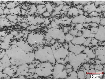
Figure ‎3-2 Scanning electron microscope through-thickness microstructure of as-received DP500 etched by Nital 2%; ferrite is dark gray and martensite is light gray. ... 37

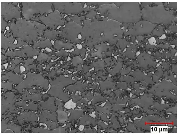
Figure ‎3-3 Optical through-thickness microstructure of as-received DP600 etched by Nital 2%; ferrite is etched in light gray and the other constituents are in dark gray/black. ... 37

Figure ‎3-4 Optical through-thickness microstructure of as-received DP600 etched by Picral 4%; bainite is etched in black and the other constituents are in gray. ... 38

Figure ‎3-5 Optical through-thickness microstructure of as-received DP600 etched by LePera; martensite is etched in white and the other constituents are in gray/black. ... 38

Figure ‎3-6 Analysis of a micrograph in image analysis software ... 39

Figure ‎3-7 Distribution of grain size for martensite islands in the DP500 steel ... 41

Figure ‎3-8 Distribution of grain size for martensite islands in the DP600 steel ... 41

Figure ‎3-9 EDS maps and distribution of Mn (red), Cr (turquoise) and Si (blue) in a through-thickness microstructure of DP500 steel. ... 43

Figure ‎3-10 EDS maps and distribution of Mn (red), Mo (yellow), Cr (turquoise) and Si (blue) in a through-thickness microstructure of DP600 steel near the surface of the sheet. ... 44

Figure ‎3-11 EDS maps and distribution of Mn (red), Mo (yellow), Cr (turquoise) and Si (blue) in a through-thickness microstructure of DP600 steel near the centre of the sheet. ... 45

Figure ‎3-14 The true flow curve of DP500 steel ... 49

Figure ‎3-15 The true flow curve of DP600 steel ... 49

Figure 3-16 Voids in the through-thickness microstructures of (a) DP500 and (b) DP600 steels close to the necking area deformed by the standard uniaxial tensile test. ... 52

Figure ‎4-1 Analytical flow curves of (a) ferrite and (b) martensite in DP500 steel... 56

Figure ‎4-2 Analytical flow curves of (a) ferrite, (b) martensite and (c) bainite in DP600 steel ... 57

Figure ‎4-3 Analytical flow curve of combination of ferrite and bainite ... 58

Figure 4-4 Digimat-FE analysis tree ... 59

Figure ‎4-5 Determination of morphological parameters of the inclusion phases in Digimat-FE. . 60

Figure ‎4-6 RVE generation in Digimat-FE: “RVE visualization” tab ... 61

Figure ‎4-7 RVE information in Digimat-FE: “RVE global data” tab ... 62

Figure ‎4-8 RVE information in Digimat-FE: “RVE phase data” tab ... 62

Figure ‎4-9 Definition of loading Digimat-FE loadings stage, a) definition of mechanical loading and boundary condition, b) definition of loading parameters. ... 63

Figure ‎4-10 Determination of solving parameters in Digimat-FE and exporting the finite element problem to ABAQUS ... 64

(11)

Figure ‎5-1 RVEs based on real microstructures generated by (a) Uthaisangsuk et al [35], (b) Paul [39], (c) Ramazani et al [40] and (d) Digimat for this research. ... 68 Figure ‎5-2 Size distribution of martensite in the RVE (Actual) and real microstructure (Reference)

... 68 Figure ‎5-3 Micromechanical modeling results for DP500 steel with 11 martensite islands inside

the RVE: (a) RVE, (b) distribution of martensite in the RVE, (c) distribution of von Mises stress in the RVE at ε≈0.12, (d) distribution of equivalent strain in the RVE at ε≈0.14, (e) flow curve of RVE and (f) numerical and experimental flow curves of DP500 steel. ... 71 Figure ‎5-4 Micromechanical modeling results for DP500 steel with 14 martensite islands inside

the RVE: (a) RVE, (b) distribution of martensite in the RVE, (c) distribution of von Mises stress in the RVE at ε≈0.12, (d) distribution of equivalent strain in the RVE at ε≈0.14, (e) flow curve of RVE and (f) numerical and experimental flow curves of DP500 steel. ... 76 Figure ‎5-9 (a) Tensile toughness of the DP500 steel as measured under the experimental flow

curve and predicted using RVEs of different sizes, and (b) with an enlarged scale. ... 78 Figure ‎5-10 Micromechanical modeling results for DP600 steel with 11 martensite islands inside

(12)

Figure ‎5-13 Micromechanical modeling results for DP600 steel with 26 martensite islands inside the RVE: (a) RVE, (b) distribution of martensite in the RVE, (c) distribution of von Mises stress in the RVE at ε≈0.125, (d) distribution of equivalent strain in the RVE at ε≈0.15, (e) flow curve of RVE and (f) numerical and experimental flow curves of DP600 steel. ... 84 Figure ‎5-14 Micromechanical modeling results for DP600 steel with 32 martensite islands inside

the RVE: (a) RVE, (b) distribution of martensite in the RVE, (c) distribution of von Mises stress in the RVE at ε≈0.125, (d) distribution of equivalent strain in the RVE at ε≈0.15, (e) flow curve of RVE and (f) numerical and experimental flow curves of DP600 steel. ... 86 Figure ‎5-16 (a) Tensile toughness of the DP600 steel as measured under the experimental flow

curve and predicted using RVEs of different sizes, and (b) with an enlarged scale. ... 87 Figure ‎5-17 Effect of mesh size on modeling results for DP500 steel with 26 martensite islands

inside the RVE: (a) flow curves of RVEs and (b) numerical and experimental flow curves of DP500 steel. ... 90 Figure ‎5-18 Effect of mesh size on modeling results for DP600 steel with 26 martensite islands

inside the RVE: (a) flow curves of RVEs and (b) numerical and experimental flow curves of DP600 steel. ... 91 Figure ‎5-19 (a) RVE of DP500 with 26 martensite islands, (b) distribution of equivalent strain

inside the RVE at ε=0.14 with mesh size of 0.025 µm, and (c-f) cross-sections of the RVE at different depths. The depths of sections are shown on the RVE. ... 92 Figure ‎5-20 (a) RVE of DP500 with 26 martensite islands, (b) distribution of equivalent strain

(13)

Figure ‎5-28 Flow curves of the matrix: ferrite in DP500 steel and ferrite+bainite in DP600 steel as predicted by Digimat software ... 101 Figure ‎5-29 (a) 2D RVE of DP500 steel with 42 martensite islands, and (b) size distribution of

martensite islands inside the RVE (Actual) and size distribution of martensite in the real microstructure (Reference) ... 101 Figure ‎5-31 Distribution of strain (left) and stress (right) in DP500 RVE presented in Figure ‎5-29 at true strains of (a) 0.05, (b) 0.09, and (c) 0.14. ... 104 Figure ‎5-32 Distribution of strain (left) and stress (right) in DP600 RVE presented in Figure ‎5-30 at strains of (a) 0.04, (b) 0.09, and (c) 0.16. ... 105 Figure ‎5-33 (a) Stress concentration in the RVE of DP500 steel where martensite islands lie close

(14)

List of Appendices

Appendix A

Calculation of the flow behaviour of ferrite, martensite and bainite in DP500 and DP600 steels is presented in the following. Results are used in Section ‎4.1.

(15)

List of Symbols

f ss

%C carbon content of ferrite that made solid solution

m ss

%C carbon content of martensite that made solid solution

%RA Relative Accuracy percent

b Burgers vector

C solute concentration in solid

d grain size

F Force

FM RVE deformation field

ky constant in the Hall-Petch equation

L dislocation mean free path

M Taylor factor

MS martensite start temperature

N number of measured grains

N normal to initial RVE boundaries

n normal to current RVE boundaries

PM Piola-Kirchhoff stress tensor

s standard deviation

V0 volume of undeformed RVE

Vf volume fraction of ferrite

Vm volume fraction of martensite

X initial position vector of RVE

x actual position vector of RVE

Γ current RVE boundaries

Γ0 initial RVE boundaries

γ shear strain

Δσc contribution of carbon solid solution hardening in flow stress

(16)

ε von Mises effective strain

µ shear modulus

ρ dislocation density

σ0 friction stress opposing the movement of dislocations

σf flow stress

σm Cauchy stress

σSSS flow stress associated with solid solution strengthening

σy yield strength

(17)

1 Introduction

1.1 Motivations for Dual Phase Steels

Most of the current passenger vehicles operate on fossil fuels which tend to create

economic and ecological challenges. One way to decrease fuel consumption is to reduce

vehicle weight and this can be done by using stronger and thinner sheets in the vehicle

body so as not to compromise passenger safety. Reducing the thickness of body parts and

simultaneously preserving occupant safety requires a grade of sheet metal with an

excellent combination of strength and formability such as dual phase steels.

As is shown in Figure 1-1, dual phase steels cover wide ranges of elongation and strength

which means that there are grades of dual phase steels with varying combinations of

strength and formability which can be used for different automotive body. The

designation of dual phase steels includes a prefix DP as an abbreviation for dual phase and

a number which represents the ultimate tensile strength of the steel. For instance, DP600

steel is a type of dual phase steel with an ultimate tensile strength that is at least 600

MPa. DP500, DP600, DP780 and DP980 are the more common industrial grades of dual

phase steels.

With their superior and wide range of combination of strength and ductility, dual phase

steels have gradually increased in market share. For instance, as is shown in Figure 1-2,

According to World Auto Steel’s Future Steel Vehicle (FSV) program, more than 30% of the

future electric and hybrid vehicle bodies is expected to be made from three grades of dual

phase steel.

In addition to a superior combination of strength and ductility, dual phase steels have

attracted attention in the sheet metal forming industry due to their specific characteristics

such as continuous yielding, low yield to tensile strength ratio, high initial work hardening

(18)

Figure 1-1 Total elongation of different steels as a function of (a) yield strength and (b)

ultimate tensile strength. HSS: high strength steel; AHSS: advanced high strength steel; IF:

interstitial free; BH: bake hardened; HSLA: high strength low alloy; TRIP: transformation-induced

plasticity; DP: dual phase; MS: martensitic steel. [1]

Figure 1-2 Application of different types of steel in the 2015-2020 electric and hybrid vehicles

(19)

1.2 Micromechanical Modeling of Flow Behaviour

Microstructural parameters have a significant influence on the flow behaviour of

materials; however, microstructural features are not considered in phenomenological

finite element (FE) modeling of materials. To investigate the influence of microstructural

features on flow behaviour, microstructure-based finite element models are developed.

These models are known as micromechanical models.

In all mechanical modeling, elastic and plastic parameters such as Young’s modulus,

Poisson’s ratio, yield stress, hardening modulus and hardening exponent are considered.

In micromechanical models, chemical composition and volume fraction of phases, grain

size and dislocation-based parameters are also taken into account. Hence,

micromechanical models are able to predict the effects of solid solution hardening, grain

size refinement and dislocations on the strength and ductility of sheet metal.

As it is shown in Figure ‎1-3, depending on the goal, modeling can be carried out at different scales. Micromechanical modeling of the flow curve can be carried both at a

micro and macro-scale. It means that in micromechanical modeling, there is a bridge to

relate the micro and macro scale flow behaviour of material. The micromechanical

modeling technique that is used in this research is based on the representative volume

element (RVE) method which is described in Section ‎2.4.

(20)

1.3 Objective of the Research

The objective of this research is to predict the flow behaviour of DP500 and DP600 dual

phase steels using a micromechanical model. The representative volume element (RVE)

method was used for micromechanical modeling. Microstructural materials parameters

such as chemical composition, volume fraction and morphology of phases as well as

effects of modeling parameters including RVE and mesh size and element type have been

investigated in this research.

1.4 Structure of the Dissertation

A brief description of the contents of each chapter is presented in the following:

Chapter 2 presents a literature review on the processing, strengthening mechanisms and

flow behaviour of dual phase steels. Also, fundamentals of micromechanical modeling

using the RVE method and the key points of micromechanical modeling of dual phase

steels are described in this chapter. Finally, there is a brief review of the Digimat software

which was used for micromechanical modeling.

Chapter 3 describes characterization of as-received DP500 and DP600 steel sheets

including quantitative metallography, chemical analysis, flow behaviour and analysis of

voids in the microstructure of deformed specimens.

Chapter 4 exhibits the general procedure that was used in this thesis for micromechanical

modeling of dual phase steels using the RVE method.

Chapter 5 includes the results of this research and discusses the merits of this work. The

numerical flow curves that were obtained for DP500 and DP600 steels are compared with

the corresponding experimental flow curves. Also, influences of the RVE size and mesh

size on the numerical results are discussed in this chapter.

(21)

2 Literature Survey

2.1 Introduction to Dual Phase Steels

Dual phase steels were introduced in the 1960s [4] and started to be used in the

manufacturing industry in the 1970s. Their greater combination of strength and ductility

compared to conventional steels encouraged the industries to support research on

processing and microstructure-properties relationship of dual phase steels. The

microstructure of dual phase steels consists of ferrite as the soft matrix and martensite as

the hard phase, and small amounts of bainite may also be present. Ferrite and martensite

are responsible for plastic deformation and strengthening of dual phase steels,

respectively.

Commercial dual phase steels are produced by an intercritical annealing heat treatment in

the (α + ϒ) region of the iron-cementite phase diagram followed by rapid quenching to

room temperature. Quenching must be sufficiently fast to avoid the diffusion and

formation of other structures such as pearlite and bainite. However, in bainite-assisted

dual phase steel, the steel is quenched to a certain temperature, an isothermal heat

treatment is carried out to form bainite and a second rapid quench cools the steel to room

temperature. The martensite volume fraction varies in different grades of dual phase

steel. For instance, as it is shown in Figure 2-1, the martensite fraction in a typical DP500

and DP780 steel is approximately 10 vol% and 20 vol%, respectively; however, in a DP980

steel, the volume fraction of martensite is more than 30 vol% in order to provide sufficient

strength to the steel. The martensite content in dual phase steels determines the

intercritical annealing temperature. According to the lever rule, greater amounts of

austenite are formed at higher intercritical annealing temperatures which transforms to

(22)

Figure 2-1 Microstructure of (a) DP500, (b) DP780 and (c) DP980 steels including ferrite grains

(dark matrix) and martensite (bright phase) [5].

During processing of dual phase steels, different alloying elements are used in solid

solution to increase the strength and hardness of the steel. Silicon, manganese,

chromium, and molybdenum are the typical alloying elements in dual phase steels. Silicon

affects the chemical composition of austenite by accelerating the migration of carbon

atoms from the ferrite to the austenite during intercritical annealing [6]. Manganese is

used to enhance hardenability of dual phase steels [7]. Chromium and molybdenum

reduce the critical cooling rate of austenite for martensitic transformation [8,9]. Other

elements such as vanadium and titanium may be added to form carbide and nitride

precipitates that can increase the strength of the steel by precipitation hardening [10].

These precipitates limit the movement of the ferrite-austenite interface during quenching

and enhance the martensite formation [11].

2.2 Strengthening Mechanisms in Dual Phase Steels

The microstructure of commercial dual phase steels includes ferrite and martensite.

Depending on the heat treatment cycle, it may also include same bainite. The influence of

strengthening mechanisms in ferrite, martensite and bainite on the flow stress of dual

(23)

2.2.1 Ferrite

Ferrite is the interstitial solid solution of carbon in body centered cubic (BCC) iron. It is the

predominant phase in most low carbon steels including high strength low alloy steels

(HSLA) and dual phase steels (DP). The ferrite grain size has a significant influence on the

yield strength of dual phase steels. The influence of grain size on yield strength is

described by the Hall-Petch relationship which was successively developed by Hall [12]

and then Petch [13]:

2 1 y 0 y =σ +k d

σ ‎2-1

where d is the grain diameter, σy is the yield stress, σ0 is the friction stress opposing the

movement of dislocations in the grains and ky is a constant. The mean ferrite grain size in

advanced dual phase steels is reduced to less than 10 µm which remarkably enhances the

flow stress.

Solid solution hardening is another strengthening mechanism that enhances the flow

stress of ferrite. In dual phase steels, manganese is the dominant alloying element which

has a notable influence on strengthening of the steel. Solid solution strengthening

depends on the solute concentration as follows [14]:

n SSS=kc

σ ‎2-2

where c is the solute concentration, k is a constant, and 0.5<n<0.67.

2.2.2 Martensite

During processing of dual phase steels, the steel is quenched from the intercritical

annealing temperature to room temperature. During this heat treatment, the intercritical

austenite transforms to martensite by a diffusionless phase transformation. The

mechanical strength of martensite primarily depends on its carbon content [14][15]. The

dependence of martensite hardness on the carbon content of the steel is shown in

Figure ‎2-2. Also, Figure ‎2-3 presents the yield strength of martensite as a function of martensite carbon content. Similar to ferrite, solid solution hardening is a strengthening

(24)

Figure ‎2-2 Hardness of martensitic steel as a function of carbon content [16]

Figure ‎2-3 Dependence of martensite yield strength on martensite carbon content [17]

The mechanical properties of dual phase steels significantly depend on the volume

(25)

ductility of dual phase steels improves with a finer dispersion of martensite islands rather

than a coarse, banded or laminated martensite in the microstructure [20,23].

Martensite strength has a crucial role in the strengthening of dual phase steels. Since the

martensite phase is a hard phase, the external loads are transferred to the martensite

from the soft ferrite matrix. Hence, by increasing the volume fraction of martensite the

yield and ultimate tensile strengths of dual phase steel increase [24]; however, it was

reported that 55 vol% of martensite resulted in the greatest strength but beyond that a

strength reduction was observed [20]. This behaviour is explained by the decreasing

carbon content of martensite when its volume fraction increases which leads to softening

of the martensite. Dependency of martensite strength on the martensite carbon content

was described by square-root [25] and cube-root [26] equations; however, it has also

been simply described by a linear equation by several authors [17,21,27]. In dual phase

steels with a high-carbon martensite phase, under external loading, the martensite

remains elastic and only the ferrite phase deforms plastically; therefore, the steel

deformation is more comparable to that of alloys that are hardened with ultra-high

strength particles [17].

2.2.3 Bainite

As it is shown in Figure ‎2-4, bainite forms by decomposition of austenite at a temperature

above the martensite start temperature (Ms) and below the pearlite formation

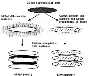
temperature. As it is presented in Figure ‎2-5, bainite is a combination of plate-shaped ferrite and carbides. Bainite is presented in two forms: lower-bainite and upper-bainite.

Lower-bainite forms at temperatures closer to the Ms while upper-bainite forms at higher

temperatures. The difference between upper and lower bainite occurs due to the

dependence of the diffusion rate of carbon on the temperature at which bainite is

forming. At higher temperatures, carbon diffuses faster from the newly formed ferrite to

the residual austenite between the ferritic plates and forms large carbides. At low

temperatures, diffusion of carbon is slower; hence, carbides precipitate inside the ferrite

(26)

consists of cementite and dislocation-rich ferrite. The strength of this ferrite with high

concentration of dislocations is greater than that of ordinary ferrite. The hardness of

bainite is between that of pearlite and martensite [28].

Figure ‎2-4 Schematic temperature-time-transformation (TTT) diagram showing the different

domains of transformations in steel [29]

(27)

2.3 Yielding and Work Hardening Behaviour of Dual Phase Steels

The yield point is the stress at which a material begins to deform plastically. As is shown in

Figure 2-6, low carbon steels generally exhibit yield point elongation. The yield point

phenomenon includes upper and lower yield points in the tensile stress-strain curve

followed with oscillations of the flow stress. In low carbon steels, dislocations are locked

by the interstitial carbon atoms. The shear stress required to cause dislocation movement

inside the grain is less than the shear stress necessary to unlock them, and this causes a

sharp drop in stress at the yield point. The following oscillations, known as Lüders bands,

continue until there are sufficient mobile dislocations to start continuous work hardening.

Figure ‎2-6 Schematic presentation of yield point phenomenon in low carbon steels

As it is shown in Figure 2-7(a), the yield point phenomenon is not usually observed in dual

phase steels and the flow curves of dual phase steels exhibit continuous yielding due to

the processing of dual phase steels. Austenite and martensite have face centered cubic

(FCC) and body centered tetragonal (BCT) crystal structures, respectively. Hence, a volume

expansion occurs during the austenite to martensite phase transformation [31]. This

volume expansion introduces plastic deformation and therefore, as it is shown in

(28)

increasing the volume fraction of martensite the number of the newly generated

dislocations increases. These dislocations are not locked by the interstitial carbon atoms.

Hence, at the yield point, they can move immediately thus producing to make a smooth

flow curve.

Figure ‎2-7 (a) Continuous yield behaviour in dual phase steels and (b) mobile dislocations at the

ferrite/martensite interface in dual phase steels [32]

Work hardening, also known as strain hardening, is the strengthening of metals by plastic

deformation. This strengthening occurs due to the movement and generation of

dislocations within the crystal structure. Work hardening starts in materials after yielding

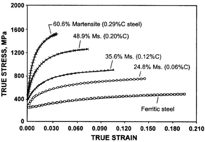
occurs. Figure 2-8 shows that work hardening in dual phase steels significantly depends on

the volume fraction of martensite. The work hardening rate is reported to be greater in

(29)

Figure 2-8 True stress-strain curve of a ferrite-martensite steel with 1.5 wt% Mn and different

carbon contents annealed at 760 °C [34]

2.4 Micromechanical Modeling Using the Representative Volume Element

Method

In the micromechanical modeling, the microstructural features of a material are

presented in a finite element (FE) model through a representative volume element (RVE).

An RVE is a small volume of microstructure that has the general characteristics of the

whole microstructure and over which modeling of specific characteristics is carried out.

The results of the RVE modeling investigations should properly describe the

characteristics of the whole microstructure. As presented in Figure ‎2-9, micromechanical modeling of flow behaviour of a material using the RVE method consists of four steps.

These steps are described in Sections ‎2.4.1 to ‎2.4.4.

Figure 2-9 Four steps of micromechanical modeling of flow behaviour using the RVE method

Definition of the RVE

Definition of flow behaviour

of each phase

Application of boundary conditions and

simulation of deformation

(30)

2.4.1 Definition of the RVE

The RVE-based micromechanical modeling technique is an approach to predict the

mechanical behaviour of materials using their microstructural features. An RVE is a small

volume of microstructure which is able to adequately represent the essential features of

the whole microstructure. It is expected that the RVE modeling method is able to

represent the overall macroscopic behaviour of the material which means that the RVE

acts as a bridge between the micro-scale and macro-scale properties of material.

A suitable RVE will have an average the same microstructural parameters as the overall

microstructure, such as volume fraction, morphology and randomness of the phases.

Hence, an RVE should be sufficiently large to include the essential microstructural

characteristics. On the other hand, the RVE size should be as small as possible so that the

states of stress and strain can be approximately considered as homogeneous in the whole

RVE. Also, a smaller RVE requires less computational resources such as computer memory

and calculation time to simulate the deformation. An advantage of micromechanical

modeling using the RVE method is that the RVE provides a detailed description of the

stress and strain distributions and their evolution in the microstructure during a metal

forming process [35–37].

A basic RVE can be defined using a simple cell model or it can be more complicated by

using a real microstructure. The RVE can also be defined in two dimensions (2D) or three

dimensions (3D). Al-Abbasi carried out micromechanical modeling of dual phase steels

using 2D and 3D cell models as the RVEs [38]. Figure ‎2-10 shows three cell models that were used by Al-Abbasi. He considered the martensite phase as circles and spheres in the

2D and 3D RVEs, respectively. The size of the circles and spheres in each cell was

(31)

Figure 2-10 Two-dimensional cell models: (a) square array, (b) stacked hexagonal array and

(c) three-dimensional array of stacked hexagonal cylinders [38].

2D and 3D RVEs can also be generated based on real microstructures. In the case of dual

phase steels, martensite and ferrite can be clearly distinguished due to the color contrast

between ferrite grains and martensite islands in a micrograph. The images from the actual

microstructure, with two different colors for ferrite and martensite, can be converted to a

2D RVE model using different digitizing techniques. The digitized image is then discretized

in preparation for the FE simulation of the deformation process. Some examples of 2D

RVEs based on real microstructures that were generated by Uthaisangsuk et al [35], Paul

[39] and Ramazani et al [40] are presented in Figure ‎2-11.

The simplest assumption for generating a 3D RVE of a two phase material is based on

Mori–Tanaka’s approach [41]. In this approach, the second phase particles are considered

as inclusions that are distributed in a matrix representing the first phase. As can be seen in

Figure ‎2-12, Uthaisangsuk et al [35], Paul [39] and Ramazani et al [40] generated cubic RVEs of dual phase steels. They considered ferrite as the matrix and martensite as

inclusions. The numbers of ferrite and martensite cubes were determined according to

(32)

Figure 2-11 2D RVEs based on real microstructures generated by (a) Uthaisangsuk et al [35],

(33)

Figure 2-12 3D RVEs based on real microstructures generated by (a) Uthaisangsuk et al [35],

(b) Paul [39] and (c) Ramazani et al [40]

The 3D RVEs that were just mentioned were generated by different researchers based on

simplified microstructural features; however, Lewis et al [42] and Brands et al [43] produced

3D RVEs using the real microstructures as shown in Figure ‎2-13. For this purpose the 3D image of the actual microstructure was obtained by assembling multiple 2D images of the

microstructure taken at different depths. This can be done by grinding and polishing the

sample over and over and taking an image at each step or by doing a 3D reconstruction of

microstructure using 3D electron backscatter diffraction (EBSD). Brands et al [43] used the

3D EBSD technique to produce a 3D RVE of a dual phase steel. They put the sample on a

tiltable holder inside of a field emission scanning electron microscope (FESEM) equipped

with a focused ion beam (FIB) cutting system. During the investigation the sample was

tilted between two positions: FIB-cutting and the EBSD positions. After taking the EBSD

image, the FIB system milled thin layers (10 nm - 1µm) from the investigated surface of

the sample. The 3D RVE of the dual phase steel was generated by assembling the EBSD

(34)

Figure 2-13 3D reconstruction of (a) austenite phase in AL-6XN microstructure [42] and (b)

dual phase steel [43] using EBSD.

There are some advantages and disadvantages for both 2D and 3D RVEs:

 It is much easier to generate 2D RVEs from real microstructure than to produce 3D

RVEs, and they are able to take into account the microstructural morphology.

 Calculation time for 2D RVEs is less than for 3D RVEs. Ramazani et al reported that

the calculation time for a 2D RVE based on a real microstructure took 30 min

whereas it took 240 min for a simple cubic 3D RVE [40].

 2D modeling has less complexity and lower computational cost compared to 3D

modeling; however, comparing the experimental and predicted results has shown

that 2D modeling underestimates the flow behaviour of dual phase steels but 3D

modeling results correlated very well with experimental results [39][40].

2.4.2 Definition of Flow Behaviour of Each Phase

To determine the flow behaviour of ferrite, martensite and bainite in dual phase steels, a

dislocation based model was developed by Rodrigues and Gutierrez [44] which has been

used by many researchers [35–37,39,40,45–49]. The development of this model is

explained in the following.

As illustrated by Gil-Sevillano [50], the orientation factor, M, relates the macroscopic flow

stress, σ, and the critical resolved shear stress, τ, and the plastic strain, ε, to the amount of

(35)

dγ dε M Mτ σ  

 _‎_2-3

From Equation ‎2-3, the macroscopic work hardening rate relates to the microscopic material parameters by:

dε dM τ dγ dτ M dε

dσ _ 2 _ ‎2-4

where dτ_dγ represents the microscopic hardening rate of the crystalline element. The

effect of strain on orientation variation is presented by the second term in Equation ‎2-4.

The classic relationship between the flow stress and dislocation density is:

p αMμb σ

Δσ σ

σ_f  ₀  ₀ ‎2-5

where α is a constant, M is the Taylor factor, µ [MPa] is the shear modulus, b [m] is the

Burger’s vector, and p is the dislocation density.

The first term in Equation ‎2-5 takes into account the contribution of the lattice friction and

the elements in solid solution. For a series of different steels with microstructures

containing ferrite, pearlite, bainite and martensite with different levels of carbon content,

the following expression for σ0 was suggested by Buessler [51]:

ss 0=77+80%Mn+750%P+60%Si+80%Cu+45%Ni+60%Cr+11%Mo+5000N

σ ‎2-6

All the elements are assumed to be homogeneously distributed in each phase.

The second term in Equation ‎2-5 is expanded based on dislocation density. Evolution of the dislocation density with strain during the deformation can be expressed as [52]:

p k bL 1 dγ dp dγ dp dγ dp r recovery

stored  

 ‎2-7

where kr is a constant and L is the dislocation mean free path. From Equation ‎2-7 and

considering p0 as the initial dislocation density and assuming that L is constant, the

(36)



1 exp( kM )



p exp( k M ) k

k αMμb

Δσ _r ₀ _r

r



  

 

 with

bL 1

k ‎2-8

So the equation for Δσ can be written as:

L k ε) Mk exp( b αMμ Δσ r r -1

 ‎2-9

Since the two terms in the Equation ‎2-5 are defined, the total approach for determination

of the flow curve of each phase is [44]:

L × k ε) Mk exp( 1 × b × μ × M × α + Δσ + σ = σ r r c 0

-- ‎2-10

where σ is the true flow stress for a true strain of ε.

The first term σ0 takes care of the effects of substitutional alloying elements as presented

in Equation ‎2-6. The second term, Δσc, describes the strengthening due to interstitial

carbon; however the strengthening effect of carbon in ferrite is not the same as in

martensite. Therefore Δσc is calculated differently for ferrite and martensite [44]:

) (%C × 5000 = Δσ f SS f

c ‎2-11

161 ) (%C × 3065 = Δσ m SS m

c - ‎2-12

where f

SS

%C and m SS

%C are the carbon wt% in ferrite and martensite, respectively.

(37)

Table 2-1 The values of the parameters in the third term of Equation ‎2-10

M: Taylor Factor M=3

µ: Shear Modulus µ= 80000 MPa

b: Burger’s vector b=2.5×10-10m

α: constant α=0.33

Kr: Recovery Rate _{For ferrite (}

dα 10 kr 5



 ), where dα is the

ferrite grain size [53] For martensite (kr=41) [53]

For bainite, (kr 10 5_dγ



 ), where dϒ is the prior

austenite grain size [46]

L: dislocation mean free path

For ferrite (L= dα ) [53]

For martensite (L= 3.8×10-8 m) [53] For bainite (L= 2 × 10-7) [46]

For bainite the factor L is assumed to be the average distance between low angle grain

boundaries measured in random directions. Bainite laths are generally 0.2 µm wide and

therefore L is considered as the value presented in Table ‎2-1. Kr for bainite is considered to

relate to the prior austenite grain size as shown in Table ‎2-1. Using the prior austenite grain size seems to give a better estimation since using the bainitic ferrite lath width in the

Hall-Petch equation results in an excessively high strength contribution [46]. Hence, the

prior austenite grain size needs to be identified to determine the flow behaviour of

bainite.

For bainite, the effect of dislocation strengthening is more significant than the

strengthening effect by carbon solid solution [29]. Δσc for bainite is considered to be a

function of the prior austenite grain size and transformation temperature. The

transformation temperature dependency comes from the fact that Δσc depends on

(38)

amount of dislocation increases. Prior austenite grain size also affects the Δσc of bainite as

it can affect the bainitic transformation temperature and kinetics [29][46].

The hardness of bainite grains was reported to be equal to the hardness of ferrite and

martensite according to the mixture rule [37]:

m m c f f c b

c=Δσ V +Δσ V

Δσ ‎2-13

where V is the volume fraction of phases in the dual phase steel microstructure.

2.4.3 Application of Boundary Conditions and Solving the Problem

Kouznetsova [54] described the theory of boundary conditions for micromechanical

modeling of multi-phase materials in her PhD thesis. A summary of this theory is

presented in the following.

Appropriate boundary conditions such as loading and constraints should be applied to an

RVE to investigate the flow behaviour of RVE in a specific condition. This will define a

problem in continuum solid mechanics which will be solved by the finite element method.

The RVE deformation field in a point with initial position vector X_{(in the reference}

domain of V0) and the actual position vector x



(in the current domain V) is described by

the deformation gradient tensor:

c 0m

m ( x)

F    ‎2-14

where the gradient operator ∇0m is taken with respect to the reference microstructural

configuration. Also the RVE is in a state of equilibrium, which mathematically is reflected

by an equilibrium equation in terms of the Cauchy stress tensor σm. It can be described in

terms of the first Piola-Kirchhoff stress tensor of Pm which is presented below:

0 σ_m m   

 in V, or

0 Pc m 0m   

 in V0

‎ 2-15 1 c m m m

m det(F )σ (F )

(39)

where mis the gradient operator with respect to the current deformation of the

microstructure. By imposing the macroscopic deformation gradient tensor FM on the

microstructural RVE through a specific approach, the actual macro-to-micro transition is

possible. The simplest is to use the Taylor (or Voigt) assumption which assumes that all of

the microstructure constituents are subject to a constant deformation which is the same

as the macroscopic deformation. Another assumption is that of Sachs (or Russ) which

assumed that an identical constant stress is applied to all the components. These

simplified assumptions do not really reflect the actual deformation of the microstructure.

Many of the accurate averaging strategies require the solution of the detailed

microstructural boundary value problem to transfer the given macroscopic variables to

the microstructural RVE via the boundary conditions. Classically, three types of RVE

boundary conditions are used, i.e. prescribed displacements, prescribed forces and

prescribed periodicity.

In prescribing displacement boundary conditions, the position vector of a point on the RVE

boundary in the deformed state is defined as:

X F

x _M 

 

 with X_onΓ 0 ‎2-17

where Γ denotes the undeformed boundary of the RVE and F₀ M the macroscopic

deformation gradient tensor on the microstructural RVE. This kind of condition prescribes

a linear mapping of the RVE boundary.

The traction boundary conditions, are described as:

0 c M m Γ on .P N = p or Γ, on .σ n = t     ‎ 2-18

(40)

Periodic boundary conditions were introduced based on the assumption of

microstructural periodicity [54]. The periodicity conditions of the RVE are presented in a

general form in Equation ‎2-19 which represents a periodic deformation:

) (    _ _ _ _ X X F x

x  _M   ‎2-19

From Equation ‎2-19 and Figure ‎2-14, the parts of RVE boundary

Γ

₀and

Γ

₀are defined in

such a way that NN at corresponding points on

Γ

0and



0

Γ

.

The periodic boundary condition can be expressed as:

1

4 x

x x

x_T _B  

    1 2 x x x xR L

    _ _ _ 1 4 2

3 x x x

x   

‎ 2-20

Where xT

 , xB

 , xL



, and xR



, are the position vector at the top, bottom, left, and right,

boundary of the RVE, respectively.

x



_i (i= 1, 2, 3, 4) are position vectors of the corner

points 1, 2, 3, and 4, in the deformed state, respectively. These position vectors are

described according to:

i M i F X

x   and i=1,2,3,4 ‎2-21

(41)

It has been reported [55][56] that the periodic boundary condition provides a better

estimation of the overall properties of the microstructure compared to the prescribed

displacement and prescribed traction boundary conditions.

2.4.4 Homogenization

Kouznetsova [54] also described the theory of homogenization for micromechanical

modeling of multi-phase materials. A summary of this theory is provided in the following.

Homogenization is a technique that relates the micro-scale behaviour of a material to its

macroscopic behaviour. Computational homogenization technique has proven to be a

valuable tool to establish non-linear micro-macro structure-property relations. In

homogenization, the material is assumed to be sufficiently homogeneous at the

macro-scale, but heterogeneous at the micro-scale due to the existence of inclusions, grains,

interfaces, cavities, etc.

Two approaches are proposed to describe the periodicity of the inhomogeneity in the

microstructure: global periodicity and local periodicity which are schematically shown in

Figure ‎2-15. In the global periodicity approach, the same inhomogeneity is assumed to repeat itself throughout the whole microstructure. The local periodicity approach is

preferred since it allows a microstructure to include a variety of inhomogeneities with

different morphologies that are repeated at individual macroscopic points. Hence, it

allows the modeling of the effects of a non-uniform distribution of the microstructure on

(42)

Figure ‎2-15 Schematic representation of a macrostructure with (a) a locally and (b) a globally

periodic microstructure [54].

It has been reported that a first order computational homogenization technique can be

used for RVE problems [40][54][57]. In a homogenization procedure macroscopic and

microscopic quantities are shown by “M” and “m”, respectively. As it is designated in

Figure ‎2-16, the first-order homogenization is carried out in three steps:

 The deformation tensor, FM, is calculated for every material point, i.e. the

integration points of the macroscopic mesh in a FE model.

 FM of a macroscopic point is used to formulate the boundary conditions which are

imposed on the RVE located on that point which results in the deformation of the

RVE.

 The stress tensor, PM, of the initial macroscopic point is obtained by averaging the

resulting RVE stress field over the volume of the RVE.

The numerical stress-deformation relationship at the macroscopic point is the result of

this procedure. Furthermore, the local macroscopic consistent tangent is obtained based

(43)

Figure ‎2-16 Schematic representation of first-order homogenization [54]

In first order homogenization, coupling of the macroscopic and microscopic deformation

and stress is carried out by application of integral averaging theorems. The integral

averaging expressions were first proposed by Hill (1963) [58] for small deformations and

developed for large deformation by Hill (1984) [59] and Nemat-Nasser (1999) [60] as

follows:

Deformation It is assumed that the macroscopic deformation gradient tensor FM is the

volume average of the microstructural deformation gradient tensor Fm:



    0 0 0 0 0 0 1 1 d N x V dV F V F V m M 

 ‎2-22

where V0 is the undeformed volume of the RVE. The divergence theorem is used to

transform the volume integral over V0 of the RVE to a surface integral. The validation of

(44)

M M M M F d N X F V d N X X F V d N x x V d N x d N x V F                       



                  0 0 0 0 0 0 0 0 0 0 0 0 0 0 0 1 ) ( 1 ) ( 1 1           

 ‎2-23

where x is position vector of nodes in deformed state and X is position vector of nodes in undeformed state. n and N are the normal to the current (Γ) and initial (Γ0) RVE

boundaries, respectively.

Stress The averaging relation for the first Piola-Kirchhoff stress tensor is:

0 0 ₀ 1 dV P V P V m M 



‎ 2-24

The macroscopic Piola-Kirchhoff stress tensor PM in the microstructural quantities defined

on RVE surface is:

0 0     c m

m P for microscopic equilibrium

I X

m 

₀  for microstructure equality

) ( )

( )

( ₀ P X P ₀ X ₀ P X

P c m m m m c m m m             ‎ 2-25

By substitution of Equation ‎2-25 into Equation ‎2-24 and applying the divergence theorem and definition of the first Piola-Kirchhoff stress vector according to Equation 2.14, PM of

RVE is obtained over the surface:

c m P N

p  ‎2-26



          0 0 0 0 0 0 0 0 0 0 1 1 ) ( 1 d X p V d X P N V dV X P V P c m c m V m M    

 _‎_2-27

By considering the periodicity conditions (Equations ‎2-20 and ‎2-21) for the RVE shown in

(45)

i i

i

M fX

V

P

∑



4 , 2 , 1 0 1 

 ‎2-28

where f_i are the resulting external forces at the boundary nodes and Xi



are the position

vectors of these nodes in the undeformed state.

2.5 Key Points in RVE-based Modeling of Dual Phase Steels

Several researchers have developed RVE-based micromechanical models to predict the

flow behaviour of dual phase steels. In 1999, Huper et al [61] modeled the flow behaviour

of dual phase steel based using an FE model. They found that flow behaviour of dual

phase steels depended on volume fraction of phases and the shape of the grains. In 2000,

Ishikawa et al [62] used a body centered cubic (BCC) cell model to investigate the effects

of volume fraction and morphology of second-phase particles on deformation behaviour

of ferritic steels. The cell model proposed by Ishikawa et al accurately estimated the

tensile behaviour of ferrite-pearlite steels. In 2003, Al-Abbasi and Nemes [63,64] studied

the effects of martensite volume fraction and martensite size on strength and ductility of

dual phase steel using a cell model. After 2010, the number of publications on

micromechanical modeling of flow curves of dual phase steels notably increased.

Uthaisangsuk et al [35] suggested a 3D RVE-based micromechanical model of randomly

distributed martensite in a ferrite matrix to predict flow curves of a dual phase steel and a

TRIP steel. Marvi-Mashhadi et al [65] predicted flow curves of dual phase steels with

18-44 vol% of martensite by development of an RVE-based FE model using the actual

microstructure of dual phase steels. Sodjit et al [66] modeled the flow curves of dual

phase steel with 25-90 vol% of martensite by proposing a 2D RVE-based FE model using

actual microstructures. They also studied the effect of martensite volume fraction on the

behaviour of the flow curves of dual phase steels. Paul et al [45,67] developed 2D and 3D

RVE-based models to predict flow behaviour of a dual phase steel. Plastic strain

localization under tensile loading was studied as a pre-stage of failure. Finally, Ramazani

et al [40,49] studied the flow behaviour of dual phase steels using 2D and 3D RVE-based

Microstructural Analysis and Micromechanical Modeling of Flow Behaviour of Dual Phase Steels Using a Representative Volume Element Method

Scholarship at UWindsor

Scholarship at UWindsor

Microstructural Analysis and Micromechanical Modeling of Flow

Microstructural Analysis and Micromechanical Modeling of Flow

Behaviour of Dual Phase Steels Using a Representative Volume

Behaviour of Dual Phase Steels Using a Representative Volume

Element Method

Element Method

Microstructural Analysis and Micromechanical

Modeling of Flow Behaviour of Dual Phase Steels

Using a Representative Volume Element Method

By

Maedeh Amirmaleki

A Thesis

Submitted to the Faculty of Graduate Studies

through Mechanical, Automotive and Materials Engineering

in Partial Fulfillment of the Requirements for

the Degree of Master of Applied Science

at the University of Windsor

Windsor, Ontario, Canada

2014

Microstructural Analysis and Micromechanical Modeling of Flow Behaviour

of Dual Phase Steels Using a Representative Volume Element Method

Maedeh Amirmaleki

__________________________________________________________

Dr. D.O. Northwood

Mechanical, Automotive, & Materials Engineering

___________________________________________________________

Dr. V. Stoilov

Mechanical, Automotive, & Materials Engineering

____________________________________________________________

Dr. D. Green

, Advisor

Mechanical, Automotive, & Materials Engineering

Author’s Declaration of Originality

Abstract

Table of Contents

List of Tables

List of Figures

List of Appendices

List of Symbols

1

Introduction

2

Literature Survey





Γ

Γ

Γ

Γ

x

























∑