Robust Estimation via Measurement Error Modeling

(1)

Abstract

WANG, QIONG. Robust Estimation via Measurement Error Modeling. (Under the direction of Dr. Leonard A. Stefanski and Dr. Marc G. Genton.)

We introduce a new method to robustifying inference that can be applied in any situation where a parametric likelihood is available. The key feature is that data from the postulated parametric models are assumed to be measured with error where

the measurement error distribution is chosen to produce the occasional gross errors found in data. We show that the tails of the error-contamination model control the

properties (boundedness, redescendingness) of the resulting inﬂuence functions, with heavier tails in the error contamination model producing more robust estimators. In the application to location-scale models with independent and identically distributed

data, the resulting analytically-intractable likelihoods are approximated via Monte Carlo integration. In the application to time series models, we propose a Bayesian approach to the robust estimation of time series parameters. We use Markov Chain

(2)

ROBUST ESTIMATION VIA MEASUREMENT ERROR MODELING

by

QIONG WANG

A dissertation submitted to the Graduate Faculty of North Carolina State University

in partial fulﬁllment of the requirements for the Degree of

Doctor of Philosophy

STATISTICS

Raleigh

2005

APPROVED BY:

Dr. Leonard A. Stefanski Dr. Marc G. Genton

Chair of Advisory Committee CO-Chair of Advisory Committee

Dr. Dennis D. Boos Dr. David A. Dickey

(3)

Biography

Qiong Wang was born on December 4th, 1978 to Boren Wang and Huizhi Zhu in Kaihua, China. She graduated from No. 1 High School in Changzhou in 1996.

She received a Bachelor of Sciences degree in Applied Mathematics from Southeast University in Nanjing, China in 2000, and a Master’s of Sciences degree in Probability and Mathematical Statistics in 2002. She then joined the graduate program in the

(4)

Acknowledgements

Firstly, I would like to express my deepest appreciation to my wonderful advisors Dr. Leonard Stefanski and Dr. Marc Genton for their guidance, training and support

during this research. I feel so fortunate to have worked with them and learned from them, and I have great admiration for their intellect and work ethic.

I am grateful to the valuable suggestions and comments of Dr. Dennis Boos to

this work. My thanks also go to Dr. Bibhuti Bhattacharyya, Dr. David Dickey, and Dr. Sujit Ghosh for their warm help with various problems in my research.

I also want to thank my dear friends, Dazhe Wang, Liyun Ma, Guanjun Jiang, Xiaoni Liu, Xiang Guo, Jiajun Liu, Guozhi Gao, Huiqin Liu, Shengmao Chang, Xi Chen and Joe Boyer for their support and encouragement during these three years.

They make me feel that life is so beautiful.

(5)

List of Figures

2.1 The score function under non-invariant error models . . . 22 2.2 The score function under invariant error models when τ and are

chosen to achieve the eﬃciency 95%. . . 23 2.3 Performance of normal contamination estimators with small B . . . . 26 2.4 Performance of Laplace contamination estimators with small B . . . 27

2.5 Performance of Cauchy contamination estimators with small B . . . . 28 2.6 Boxplot of estimated degrees of freedom versus true degrees of freedom

for the t-adaptive estimators. . . 34

3.1 Boxplot of ˆα₁ for AR(1) model withα₁ = 0.5 and 10% contamination. 52 3.2 The Cauchy BMEM-estimates of the gross errors against the true

val-ues for the AR(1) model with α₁ = 0 and 10% contamination (κ= 5). 61 3.3 Monthly interest rates of an Austrian bank during 91 months. . . 65 3.4 Saving rates in the United States from the ﬁrst quarter of 1955 to the

(9)

List of Tables

2.1 Normal, Laplace, and Cauchy contamination model tuning parameters

for 85%, 90% and 95% eﬃciency at the normal location-scale model. 18

2.2 Estimated eﬃciencies relative to Huber’s Proposal 2 of location esti-mators. . . 29

2.3 Estimated eﬃciencies relative to Huber’s Proposal 2 of scale estimators. 30

2.4 Estimated eﬃciencies oft-adaptive estimators relative to Huber’s

Pro-posal 2 . . . 33

3.1 Monte Carlo average and mean squared errors of posterior mean of θ when data were generated from AR(1) with α₁ =−0.5. . . 47

3.2 Monte Carlo average and mean squared errors of posterior mean of θ when data were generated from AR(1) with α₁ = 0. . . 48

3.3 Monte Carlo average and mean squared errors of posterior mean of θ when data were generated from AR(1) with α₁ = 0.25. . . 49

(10)

3.5 Monte Carlo average and mean squared errors of posterior mean of θ

when data were generated from AR(1) with α₁ = 0.75. . . 51 3.6 Monte Carlo average and mean squared errors of posterior mean of θ

when data were generated from AR(2) with α₁ = 0.6 and α₁ = 0.3. . 53 3.7 Monte Carlo average and mean squared errors of posterior mean of θ

when data were generated from AR(2) with α₁ =−0.6 and α₁ = 0.3. 54 3.8 Monte Carlo average and mean squared errors of posterior mean of θ

when data were generated from AR(2) with α₁ = 0.3 and α₁ =−0.6. 55 3.9 Monte Carlo average and mean squared errors of posterior mean of θ

when data were generated from AR(2) with α₁ =−0.3 and α₁ =−0.6. 56 3.10 Monte Carlo average and mean squared errors of posterior mean of θ

when data were generated from MA(1) withβ₁ = 0.5. . . 57 3.11 Monte Carlo average and mean squared errors of posterior mean of θ

when data were generated from MA(1) withβ₁ = 0.8. . . 58 3.12 Correlation of true value and BMEM-estimates of the gross errors. . . 60 3.13 Monte Carlo average of posterior mean of θ for the Cauchy

BM-estimator when the data were generated from AR(1) with diﬀerent

sample sizes. . . 62 3.14 Parameter estimates obtained by ﬁtting an AR(1) model to the data

of monthly interest rate. . . 64

(11)

A.1 Robustness comparison with Huber’s Proposal 2 based on the gross

(12)

Chapter 1 Introduction and Overview

1.1 Motivation

Modern robust statistics has focused most of its attention on problems such as the estimation of location and scale in univariate and multivariate populations with nat-ural extensions to regression and autoregressive situations. Little progress has been

made in the more challenging arenas of spatial data and general stochastic processes except for certain speciﬁc techniques such as Genton’s (1998) highly-robust variogram estimator. Parametric models and likelihood methods abound for these dependent

data situations, but they are often sensitive to outliers. What is missing is a general approach to robustifying likelihood methods that is applicable in settings with just one realization, where empirical densities and distribution functions do not exist.

(13)

connected to measurement error modeling (Stefanski, 2000; Carrol et al., 1995) and

reduces to well-known contaminated normal likelihoods in certain cases. The key idea is to model the observations with a suitable structural measurement error model for the unobservable error-free data and the observed error-contaminated data. In

the usual measurement error modeling application, the errors are typically assumed to be normally distributed in order to best model the errors produced by in-control measurement methods (Fuller, 1987; Carroll et al., 1995; Cheng and Van Ness, 1999).

In the application to robustness, we alter the assumptions on the errors to reﬂect the type of data contamination for which robust procedures are designed.

This chapter is organized as follows. In Section 2 we brieﬂy review the idea of robustness and the key tools for measuring robustness. Section 3 contains a brief introduction to measurement error models. Section 4 introduces the basic idea of

this new robust estimation method based on measurement error modeling. Section 5 summarizes the two main chapters and the last chapter.

1.2 Robust Statistics

Robustness means lack of sensitivity to small departures from the idealized assump-tions, where “small” indicates either moderate deviations for all data points or large

(14)

The most popular tools for measuring robustness are the inﬂuence function and

the breakdown point (Huber 2004). The former measures local robustness and the latter measures global robustness.

Let χ_n denote a sample with n observations and T_n(χ_n) be a statistic given χ_n.

T is called a statistical functional if T_n(χ_n) −−−→n→∞ T(F), where F is a cumulative distribution function. Consider an-contaminated distribution of F, F = (1−)F+

δ_x, whereδ_x is the point mass distribution atx, then the inﬂuence function is deﬁned

as

IF(x;T, F) = lim

→0

T(F)−T(F)

.

Heuristically, it is the rate at which T(F) changes due to the contamination at the point x. If the inﬂuence function is small, then contamination at x will not

signifi-cantly change the statistical functional. Due to this interpretation, it is desirable to have a bounded or redescending influence function. The robustness property of the influence function is quantified by the gross error sensitivity:

γ∗(T;F) = sup

x |IF(x;T, F)|,

which measures the fastest rate at which an outlier can alter the value of the statistical functional. Any statistical functional with ﬁniteγ∗ is called B-robust.

The breakdown point provides a framework within which it is possible to examine

(15)

replaced with arbitrary values. The maximum bias under_m-contamination is deﬁned

as:

B(_m;T_n, χ_n) = sup|T_n(χ_n,m)−T_n(χ_n)|,

where supremum is taken over all possible values of themcontamination points. Then

the ﬁnite sample breakdown point is deﬁned as the minimum amount of contamination to cause breakdown of the statistic:

∗(T_n;χ_n) = inf{_m :B(_m;T, χ_n) = ∞}.

One intuitive interpretation of the breakdown point is the proportion of bad data a statistic can tolerate before taking on arbitrary or meaningless values.

1.3 Measurement Error Models

The classical measurement error model (Stefanski, 2000) assumes that

W_i =X_i+U_i, i= 1, . . . , n,

whereX₁, . . . , X_n are the variables of interest, which are statistically meaningful but cannot be observed directly,U₁, . . . , U_nrepresent measurement errors, andW₁, . . . , W_n

are the observable measurements of, or substitutes for, X₁, . . . , X_n. The problem is to make inference according to the model deﬁned in terms of the unobservable

X₁, . . . , X_n, given the data on W₁, . . . , W_n.

(16)

are regarded as a sequence of unknown constants, whereas in a structural

measure-ment error modelX₁, . . . , X_n are regarded as random variables.

1.4 Robust Likelihood Approach via Measurement

Error Modeling

The idea of the robust likelihood approach is to model the observation with a suitable structural measurement error model. In this formulation the unobservable error-free

data X₁, . . . , X_n, and the observed error-contaminated data are related as

W_i =X_i+τ Z_i, i= 1, . . . , n, (1.1)

where Z₁, . . . , Z_n are independent and identically distributed with common distribu-tion G(z) and independent of X₁, . . . , X_n. We have in mind error models that result in negligible errors much of the time, but produce occasional large outlying values. Thus we assume that the central modelf(x;θ) holds except for a fraction of the data that are contaminated by random errors. We accomplish this by assuming G(z) is

a mixture of a point mass at zero and a standard density in proportions 1− and

respectively

G(z) = (1−)I(0≤z) +

_z

−∞

g(x)dx, (1.2)

whereg is a standardized probability density function, e.g., normal, Laplace, Cauchy.

(17)

(1.1) the joint density of W₁, . . . , W_n is given by

f_W(w|θ, , τ) =

· · ·

f(w₁ −τ z₁, . . . , w_n−τ z_n;θ)

n

i=1

G(dz_i) (1.3)

= E{f(w₁−τ Z₁, . . . , w_n−τ Z_n;θ)}.

Note that we list the contamination parameters and τ as parameters in the model. In some cases these will be identiﬁable and the potential exists for estimating them

from the observed data. However, often they will be specified as tuning parameters and chosen to obtain a specified level of efficiency at a central, non-contaminated model.

1.5 Research Overview

In Chapter 2 we emphasize the independent and identically distributed case, and location-scale models in particular. There are two advantages to focusing on location

and scale estimation. First, robust location and scale estimation has been thoroughly studied, and hence good benchmarks are available with which to compare estimators derived from the new approach. Second, certain theoretical results can be derived

relatively simply for location and scale estimation. Our objective with Chapter 2 is to show that the measurement error approach to robustifying estimation is competitive with established robust methods. In the case that data are independent and

(18)

function property with diﬀerent types of tail behavior for the error distribution g in

(1.2). We focus on three standard distributions: normal, Laplace and Cauchy. The main result is that the heavier tails in the error contamination distribution produces better inﬂuence function property. In study of location-scale models with

indepen-dent and iindepen-dentically distributed data, we use the common approach of tuning the estimating equations derived from the robust error contamination model to achieve consistency and desired eﬃciency at the non-contaminated normal model.

Ultimately, our intention is to robustify inference in statistical models that are not easily robustiﬁed using standard approaches, such as time series models. It is such hard-to-robustify models that piqued our interest in the error modeling approach, and

this is studied in Chapter 3. In the case that data are not independent, Monte Carlo integration can be too variable to approximate the multivariate marginal likelihood (1.3). We propose a Bayesian approach to deal with the computing problem. The

Bayesian inference is carried out using Markov Chain Monte Carlo techniques. By taking the Bayesian perspective, we obtain the posterior distribution for errors and parameters of interest, which contains all the relevant information given the observed

data. This Bayesian approach not only provides robust estimation for the parameters of interest but also achieves outlier diagnostics. The identiﬁcation of outliers is based on the posterior distribution. The Cauchy error model turns out to perform best in

both robust estimation and outlier detection.

(19)

Chapter 2 Robust Estimation for

Location-Scale Models

2.1 Introduction

We have introduced the error contamination model (1.1) and the resulting mar-ginal likelihood (1.3) in the ﬁrst chapter. In particular models, there may be clever approaches for evaluating the integral in (1.3) and maximizing the likelihood L =

fW(W|θ, , τ), but in general this will be a nonstandard computational problem. For

the particular case of independent and identically distributed observationsW₁, . . . , W_n, the marginal density (1.3) simpliﬁes to

fW(w|θ, , τ) =

n

i=1

f(w_i−τ z_i;θ)G(dz_i) =

n

i=1

(20)

where now f(x;θ) denotes the marginal density of X_i, i = 1, . . . , n. Monte Carlo

integration provides a straightforward and generally applicable solution to the com-putational problem resulting in

fW(w|θ, , τ) =

n i=1 1 B B b=1

f(w_i−τ Z_b,i∗ ;θ), (2.2)

where theZ_b,i∗ are independently and identically distributed with common distribution

G.

For location-scale models with θ= (µ, σ), (2.1) becomes

f_W(w|µ, σ, , τ) =

n i=1 1 σf

w_i−τ z_i−µ σ

G(dz_i)

= n i=1 E 1 σf

w_i−τ Z_i−µ σ

,

where nowf(x) is the kernel of the location-scale family for the marginal density ofX_i, i.e., f_X(x;µ, σ) =σ−1f((x−µ)/σ). In our study of robust location-scale estimation we adopt the common approach of setting the tuning parameters to achieve desired

levels of eﬃciency at a central model, and hence we no longer listandτas parameters in the model. In this case the location-scale model version of (2.2) is

fW(w|µ, σ) =

n i=1 1 B B b=1 1 σf

w_i−τ Z_b,i−µ σ

B_−→→∞

fW(w|µ, σ). (2.3)

Inspection of the limit likelihood L=f_W(W|µ, σ) (or the Monte Carlo version L =

fW(W|µ, σ)) reveals a problem that does not arise whenτ is estimated along with the

(21)

non-invariant error-contamination model (1.1) to

W_i =X_i+τ σZ_i, i= 1, . . . , n, (2.4)

which we call the invariant error model (invariance is proved in Appendix A.1). The

relevant versions of equations (2.1)-(2.3) for the invariant error model are obtained by replacing τ with στ, and throughout the chapter we also work with the invariant version of (2.3),

f_W(w|µ, σ) =

n

i=1

1

B

b=1

1

σf

w_i−τ σZ_b,i−µ σ

. (2.5)

When the kernel f of the location-scale family and the error contamination dis-tribution are both symmetric around 0, estimates of µ derived from the likelihoods

based on (2.3) and (2.5) will be consistent. However, scale estimates will not be con-sistent in general, and we adopt the accepted strategy of adjusting the scale estimates to ensure consistency at the non-contaminated central model, which we take to be

normal, i.e., f is standard Gaussian with no error contamination. We discuss the calculation of the scale adjustment factor in the next section. For convenience, we name the new robust estimator derived from (2.3) or (2.5) as MEM-estimator.

2.2 Robust Properties from Error-Contamination

Models

(22)

Through-out we assume that the errors Z₁, . . . , Z_n are from the gross error model

Z =T Q, (2.6)

where T is distributed as Bernoulli() and Q has a symmetric standardized distri-bution. When the distribution of Q has a ﬁnite second moment, we standardize in

the usual fashion (to mean 0 and variance 1). For distributions without the requi-site moments we standardize to median 0, with scale such that Pr(−1 < Q ≤ 1) = Φ(1)−Φ(−1) ≈ 0.6827, where Φ is the standard Gaussian cumulative distribution

function. Results are presented for the common cases where Q is normal, Laplace and Cauchy.

2.2.1 Influence Function Properties

Certain of the results in this section hold for general models with independent and identically distributed data, i.e, they are not speciﬁc to location-scale models, and we present them accordingly. We make it clear where results are speciﬁc to location-scale

models.

The contaminated density is given by

h(u;θ) =

f(u−τ_θz;θ) G(dz)

= (1−)f(u;θ) +

f(t;θ)g((u−t)/τ_θ)/τ_θ dt, (2.7)

(23)

is denoted by

ψ(u;θ, , τ) = ∂

∂θlnh(u;θ). (2.8)

We write ψ(u;θ, , τ) to emphasize the dependence of the score on the tuning para-meters even though θ is the only parameter to be estimated.

Non-invariant Error Model

Our ﬁrst results for the non-invariant error model are not speciﬁc to location-scale

models and we derive them for more general models. In this case the score function (2.8) reduces to

ψ(u;θ, , τ) = ∂

∂θlnh(u;θ)

= (1−) ˙f(u;θ) +(∂/∂θ) f(t;θ)g((u−t)/τ)/τ dt (1−)f(u;θ) + f(t;θ)g((u−t)/τ)/τ dt ,

where ˙f(u;θ) = (∂/∂θ)f(u;θ). The robustness properties (bounded, redescending)

of ψ(u;θ, , τ) can be deduced from the expression above under certain regularity conditions and assumptions on the tail behavior ofg. First re-express ψ(u;θ, , τ) as

ψ(u;θ, , τ) = (1−)τ ˙

f(u;θ)/g(u/τ) +(∂/∂θ) f(t;θ)g((u−t)/τ)/g(u/τ) dt

(1−)τ f(u;θ)/g(u/τ) + f(t;θ)g((u−t)/τ)/g(u/τ) dt .

Robustness is achieved by choosing an error contamination model with heavier tails than the assumed parametric model. For such choices of g it will generally be the case (and can usually be arranged by suitable choice of g) that

lim |u|→∞

f(u;θ)

g(u/τ) = 0 and |ulim|→∞ ˙

f(u;θ)

(24)

which we now assume. It follows that the behavior of ψ(u;θ, , τ) for large u is

determined by the behavior of g((u − t)/τ)/g(u/τ) for large u, which in turn is dictated by the tail behavior of g. Two cases are of interest: polynomial-like tail behavior,

lim |u|→∞

g(u+b)

g(u) = 1; (2.9)

and exponential-like tail behavior,

lim

u→∞

g(u+b)

g(u) = exp(c1b), u→−∞lim

g(u+b)

g(u) = exp(c2b), (2.10)

for some constants c₁ and c₂.

For the case of polynomial-like tails,

lim |u|→∞

f(t;θ)g((u−t)/τ)

g(u/τ) dt= 1

and lim

|u|→∞

∂ ∂θ

f(t;θ)g((u−t)/τ)

g(u/τ) dt = 0, (2.11)

assuming that limits, diﬀerentiation, and integration are interchangeable. It follows

that when g has polynomial-like tails, lim_|_u_|→∞ψ(u;θ, , τ) = 0, i.e., ψ(u;θ, , τ) is redescending. So the non-invariant, Cauchy error contamination model yields re-descending inﬂuence curves.

For the case of exponential-like tails,

lim

u→∞

f(t;θ)g((u−t)/τ)

g(u/τ) dt =

f(t;θ) exp(−c₁t/τ) dt,

and lim

u→−∞

f(t;θ)g((u−t)/τ)

g(u/τ) dt =

f(t;θ) exp(−c₂t/τ) dt,

(25)

the limits can be interchanged with diﬀerentiation, then

lim

u→∞ψ(u;θ, , τ) =

∂

∂θ ln{mf(−c1/τ;θ)},

and

lim

u→−∞ψ(u;θ, , τ) =

∂

∂θ ln{mf(−c2/τ;θ)},

where m_f(·;θ) is the moment generating function of f(·;θ), assumed to exist. So

the non-invariant, Laplace error contamination model results in bounded inﬂuence curves.

The normal error contamination model, i.e., g is standard normal, has neither polynomial-like nor exponential-like tails, and the results above do not apply to it. In this case the tail behavior of the score function depends on the underlying model.

When the underlying true-data model in (2.3) and (2.5) is a Gaussian location-scale model, and g in (2.9) is standard normal, standard calculus arguments (in Appendix A.3) show that the score function for location diverges linearly with asymptotic slope

= 1/(σ2+τ2); and the score function for scale diverges quadratically with coeﬃcient

σ/(σ2+τ2)2. Thus the normal contamination model does not result in qualitatively robust estimation. This ﬁnding is consistent with the results in Gleason (1993) who

argues that the contaminated normal is not truly heavy tailed.

Invariant Error Model

(26)

models is that in the latter the distribution of the added errors depends on the model

parameter σ. This does not aﬀect the tail behavior of the estimating equation for µ, but it gives rise to diﬀerent tail behavior for the estimating equation for σ. In this case theσ component of the score function is

ψ_σ(u;θ, , τ) = (∂/∂σ) lnh(u;θ)

= (∂/∂σ){f(t;θ)g((u−t)/τ σ)/τ σ}/g(u/τ σ)/τ σ dt

f(t;θ)g((u−t)/τ σ)/g(u/τ σ) dt . (2.12)

In the appendix (A.4 and A.5) we show that for the case of exponential-like tails,

lim

|u|→∞ψσ(u;θ, , τ) =∞; (2.13)

and that for the case of symmetric polynomial-like tails,

lim

|u|→∞ψσ(u;θ, , τ) =

p−1

σ , (2.14)

where p is the power of the polynomial decreasing tails, i.e., g(u) ∼ u−p. Thus in

contrast to the non-invariant error model results, exponential-like tails for g yield unbounded inﬂuence curves, and polynomial-like tailed distributions forg do not give rise to redescending (to 0) inﬂuence curves for scale estimation. It is possible to

obtain redescending estimating equations for scale using the error-model approach, but doing so necessitates using nonstandard error distributions with extremely heavy tails. For example, suppose that we start with a random variable T that is Cauchy

distributed with density 1/{π(1 +t2)}, and for a ﬁxed constant k >0 deﬁne,

U =

⎧ ⎨ ⎩

eT1k −1 T ≥0,

(27)

Then the density function ofU is symmetric around 0, with

g(u) = 1

π(1 + [log(1 +u)]2k)

[log(1 +u)]k−1

1 +u , u≥0. (2.15)

The tails of this density decrease extremely slowly and thus we call it a super-heavy

tailed distribution. If the density in (2.15) is used to construct the score in (2.12), then it is shown in the appendix (A.6) that

lim

|u|→∞ψσ(u;θ, , τ) = 0. (2.16)

Breakdown Point

The influence function is a measure of local robustness, while breakdown point mea-sures global robustness when the sample has more than one outlier. We have intro-duced the definition of the finite sample breakdown point in Chapter 1. Tyler (1994)

presents some general results of the ﬁnite sample breakdown point in simultaneous estimation of location and scale parameters. For the normal and Laplace invariant error model, the theoretical score functions are unbounded for estimators of scale,

which leads to the ﬁnite sample breakdown point 1/n. The Cauchy invariant error model achieves the optimal ﬁnite sample breakdown point n/2/n.

2.2.2 Location-Scale Model Tuning Parameter

Determina-tion

(28)

ψ(w;µ, σ, , τ) denote the two-dimensional contaminated error model score function.

The system of equations in (µ, σ) _∞

−∞ψ

(x;µ, σ, , τ) 1

σ₀φ((x−µ0)/σ0) dx=

⎛ ⎝0

0 ⎞ ⎠,

has solutionµ=µ₀,σ=c(, τ, σ₀)σ₀; where for the invariant error modelc(, τ, σ₀) =

c(, τ) independent of σ₀; but for the non-invariant modelc(, τ, σ₀) depends on σ₀ in general. In order to ensure consistency at the N(µ, σ2) model, scale estimates derived from the non-invariant likelihood must be divided by c(, τ, σ) whereas estimates

derived from the invariant error model likelihood must be divided by c(, τ). The former correction factor depends on σ and thus is not feasible unless a two-step procedure is implemented. However, the correction factor for the invariant error

model does not depend on unknown parameters and need only be calculated once for a given (, τ).

Using numerical integration to evaluate the relevant likelihoods and asymptotic covariance matrices, we determined the correction factors c(, τ, σ) and c(, τ) for N(µ, σ2) data with µ= 0 and σ = 1, and then determined the asymptotic variances of the consistent estimators. Finally, we searched over values of and τ to find pairs that result in specified target asymptotic efficiencies for both µ and σ. It was not possible to achieve the specified target efficiencies (85%, 90% and 95%)

(29)

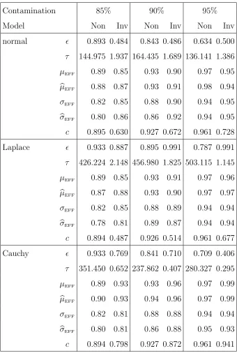
Table 2.1: Normal, Laplace, and Cauchy contamination model tuning parameters for 85%, 90% and 95% eﬃciency at the normal location-scale model.

Contamination 85% 90% 95%

Model Non Inv Non Inv Non Inv

normal 0.893 0.484 0.843 0.486 0.634 0.500

τ 144.975 1.937 164.435 1.689 136.141 1.386

µEFF 0.89 0.85 0.93 0.90 0.97 0.95

µ_EFF 0.88 0.87 0.93 0.91 0.98 0.94

σEFF 0.82 0.85 0.88 0.90 0.94 0.95

σ_EFF 0.80 0.86 0.86 0.92 0.94 0.95

c 0.895 0.630 0.927 0.672 0.961 0.728 Laplace 0.933 0.887 0.895 0.991 0.787 0.991

τ 426.224 2.148 456.980 1.825 503.115 1.145

µEFF 0.89 0.85 0.93 0.91 0.97 0.96

µ_EFF 0.87 0.88 0.93 0.90 0.97 0.97

σEFF 0.82 0.85 0.88 0.89 0.94 0.94

σ_EFF 0.78 0.81 0.89 0.87 0.94 0.94

c 0.894 0.487 0.926 0.514 0.961 0.677 Cauchy 0.933 0.769 0.841 0.710 0.709 0.406

τ 351.450 0.652 237.862 0.407 280.327 0.295

µ_EFF 0.89 0.93 0.93 0.96 0.97 0.99

µ_EFF 0.90 0.93 0.94 0.96 0.97 0.99

σ_EFF 0.82 0.81 0.88 0.88 0.94 0.94

σ_EFF 0.80 0.81 0.86 0.88 0.95 0.93

(30)

Table 2.1 continued. Table entries: Non, non-invariant error model; Inv, invariant error

model; , contaminating fraction; τ, error contamination scale; µEFF, location eﬃciency;

µEFF, Monte Carlo location eﬃciency; σEFF, scale eﬃciency; σEFF, Monte Carlo scale

eﬃ-ciency; c, scale adjustment for consistency at normal model. Standard errors for Monte Carlo eﬃciency ranged from 0.004 to 0.018 averaging approximately 0.01.

may not be accurately determined, but the computed values should yield eﬃciencies

close to the optimal. Rather than undertake a detailed assessment of the numerical methods used to determine the tuning parameters we designed a simulation study to assess the actual eﬃciencies of the computed tuning parameters. The simulation

approach has the additional advantage of allowing us to assess eﬃciency when the Monte Carlo likelihood is used for estimation. In the simulation study 2,500 N(0,1) data sets of sample sizen = 200 were generated and analyzed using the Monte Carlo

likelihood versions of the estimators (B = 800) for the various methods.

Table 2.1 displays values of , τ and the correction factors (c in the table) and the realized eﬃciencies associated with each indicated target eﬃciencies for both the non-invariant and invariant robust likelihoods. The agreement between the Monte

Carlo estimated and theoretical eﬃciencies is generally good, supporting the claim that the calculated tuning parameters result in the nominal eﬃciencies as advertised.

The large contamination proportions () and large contamination scales (τ) in Table 2.1, especially for the non-invariant cases, were unexpected. When the

(31)

have eﬃciencies less than 100% signiﬁcantly, the heavy-tailed component must be

sub-stantial. The especially large contaminating scales for the non-invariant estimators are such that the resulting score functions are similar regardless of the contaminating distribution, as shown in the next section.

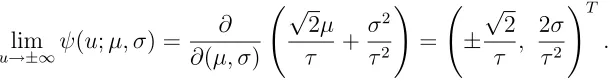
Score Function Characteristics

Score functions,ψ(u;µ, σ), for location and scale from the three non-invariant error-contaminated models are plotted in Figure 2.1. The baseline model is N(µ, σ2) with

µ = 0 and σ2 = 1. Plots (a) and (c) display the inﬂuence functions for location and scale respectively for the three types of contaminated models (normal, Laplace, Cauchy) using and τ from Table 2.1 corresponding to 95% eﬃciency. The three score functions are overlaid in 1(a) and 1(c).

As evident in the graph the three score functions are indistinguishable over the

range of u plotted. Recall that the theory indicates that the score functions are unbounded for the normal contamination model, bounded for the Laplace contami-nation, and redescending for Cauchy contamination. The fact that all of the curves

appear to redescend to 0 is an artifact of the large values of and τ in Table 2.1. For example, the location curve for the normal model has tails that diverge linearly with slope equal to 1/(1 +τ2) = 1/(1 + 136.1412)≈.000054.

(32)

contaminated with a N(0, τ2) error. That these are both unbounded is a conse-quence of the light tails of the normal contamination model. The double-dashed lines display the inﬂuence curves for the model contaminated with Laplace error,

g(u) = exp(−√2|u|)/√2. This error model has exponential tails with c₁ = −1 and

c₂ = 1. Thus, withθ = (µ, σ),

lim

u→±∞ψ(u;µ, σ) =

∂ ∂(µ, σ)

_√ 2µ

τ +

σ2 τ2

=

± √

2

τ ,

2σ τ2

_T

.

The dashed lines are the inﬂuence curves for the model contaminated with Cauchy er-ror,g(u) ={cπ(1+u2/c2)}−1, where c=0.544267. The Cauchy density has polynomial tails and thus the inﬂuence functions redescend to 0.

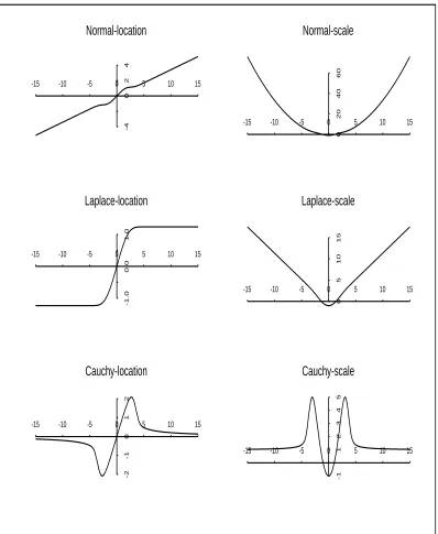
Figure 2 displays ψ(u;µ, σ) for the invariant case whenτ and are from Table 2.1

for 95% eﬃciency. The theoretical properties of the invariant score functions are read-ily observed from the graphs. The noteworthy features are the unboundedness of the score functions for the normal (location and scale) and Laplace (scale) contamination

models, and the non-redescending of the Cauchy (scale).

2.2.3 t

-adaptive Error Contamination Models

We have shown that robustness of the MEM-estimators is completely determined by the tail behavior of the speciﬁed error-contamination distribution. In practice,

(33)

Figure 2.1: The score function under non-invariant error models

-15 -10 -5 0 5 10 15

-2

-1

0

1

2

(a)

-15 -10 -5 0 5 10 15

-3

-2

-1

0

1

2

3

(b)

-15 -10 -5 0 5 10 15

-1

0

1

2

3

4

(c)

-15 -10 -5 0 5 10 15

-2

0

2

4

6

(d)

ψ(u;µ, σ) for the non-invariant case: (a) & (c) for location and scale of a normal distribution contaminated by the three types of distributions (normal, Laplace, Cauchy) when τ and are chosen to achieve the eﬃciency 95%. (b) & (d) use τ = 2, = 0.05: the solid lines for normal error, the double-dashed lines for Laplace error, the dashed lines for Cauchy error.

(34)

Figure 2.2: The score function under invariant error models whenτ and are chosen to achieve the eﬃciency 95%.

-15 -10 -5 0 5 10 15

-4

0

2

4

Normal-location

-15 -10 -5 0 5 10 15

02

0

4

0

6

0

Normal-scale

-15 -10 -5 0 5 10 15

-1.0

0.0

1.0

Laplace-location

-15 -10 -5 0 5 10 15

0

5

10

15

Laplace-scale

-15 -10 -5 0 5 10 15

-2

-1

0

1

2

Cauchy-location

-15 -10 -5 0 5 10 15

-1

12

34

5

(35)

by maximizing the likelihood with respect toµ, σ and ν.

As ν increases, the t distribution approaches a normal distribution. For ν > 30, the diﬀerences are negligible. For eachν = 1, . . . ,30, after standardization, the tuning parameters (, τ, and correction factor) associated with the desired target eﬃciency

are calculated and lead to the corresponding estimates ˆµ_ν and ˆσ_ν. The ﬁnal estimates (ˆν, ˆµ, ˆσ) is the one of the thirty sets of (ν, ˆµ_ν, ˆσ_ν) that maximizes the likelihood.

2.3 Simulation Study

We present results from simulation studies designed to illustrate features of the new robust MEM-estimators and compare them with established robust methods. Our objective is to demonstrate that the new methods are competitive with established

methods.

2.3.1 Performance for Small

B

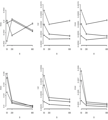
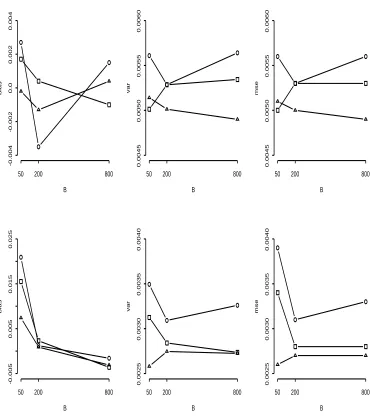
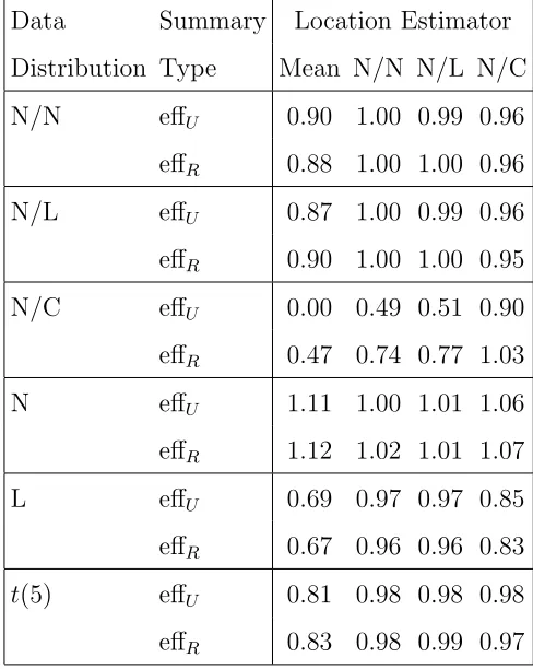
In order to decide on a suitable value ofB to be used in the Monte Carlo likelihood, we

investigated the performance (bias, variance, mean squared error) of the estimators for diﬀerent values of B (50, 200, and 800). For this preliminary study, the data were standard normal, sample size was n = 200, and 2,500 replicate data sets were

generated and analyzed.

(36)

The indicated conclusions from the simulation are: 1) location estimates are

un-biased for allB and all target efficiencies, with greater variability for estimators with lower target efficiencies; 2) scale estimates are biased high and are more variable for low values of B and low target efficiencies, although bias is negligible for B = 800,

and variability levels oﬀ for B ≥ 200; 3) the invariant estimators generally perform better than their non-invariant counterparts. Thus, in the following simulation study we use B=800.

2.3.2 Comparison with Huber’s Proposal 2

Huber’s Proposal 2 (Huber, 1964) is arguably the most used robust estimator of location and scale and we designed a simulation study to compare it to the MEM-estimators. The study was also designed to illustrate the performance of the new

invariant estimators with a small sample size (n = 25), and over a broad range of distributions. Huber’s Proposal 2 is an M-estimator with ψ function

ψ(w, µ, σ) = ⎛

⎝ χk((w−µ)/σ)

χ2_k((w−µ)/σ)−E{χ2_k(Z)} ⎞ ⎠,

where χ_k(z) = min{k,max(−k, z)} and Z ∼ N(0,1). Note that Huber’s Proposal 2 has only one tuning parameter k. Because interest lies primarily in location estima-tion, we chose k = 0.982 resulting in 90% eﬃciency for µ at the normal model; and

(37)

Figure 2.3: Performance of normal contamination estimators with small B B bias -0.003 -0.001 0.0 0.001

50 200 800

B var 0.0050 0.0054 0.0058 0.0062

50 200 800

B

mse

0.0050

0.0054

0.0058

50 200 800

B bias 0.0 0.01 0.02 0.03 0.04

50 200 800

B var 0.0 0.001 0.002 0.003 0.004

50 200 800

B mse 0.002 0.003 0.004 0.005 0.006

50 200 800

Top three plots, left to right: bias, variance and mean squared error (mse) for location

estimators. Bottom three plots, left to right: bias, variance and mse for scale estimators.

(38)

Figure 2.4: Performance of Laplace contamination estimators with small B B bias -0.004 -0.002 0.0 0.002

50 200 800

B var 0.0050 0.0055 0.0060 0.0065 0.0070

50 200 800

B mse 0.0050 0.0055 0.0060 0.0065 0.0070

50 200 800

B bias 0.0 0.02 0.04 0.06

50 200 800

B var 0.0025 0.0035 0.0045 0.0055

50 200 800

B mse 0.003 0.005 0.007 0.009

50 200 800

estimators. Bottom three plots, left to right: bias, variance and (mse) for scale estimators.

(39)

Figure 2.5: Performance of Cauchy contamination estimators with small B B bias -0.004 -0.002 0.0 0.002 0.004

50 200 800

B var 0.0045 0.0050 0.0055 0.0060

50 200 800

B mse 0.0045 0.0050 0.0055 0.0060

50 200 800

B bias -0.005 0.005 0.015 0.025

50 200 800

B var 0.0025 0.0030 0.0035 0.0040

50 200 800

B mse 0.0025 0.0030 0.0035 0.0040

50 200 800

estimators. Bottom three plots, left to right: bias, variance and mse for scale estimators.

(40)

Table 2.2: Estimated eﬃciencies relative to Huber’s Proposal 2 of location estimators.

Data Summary Location Estimator Distribution Type Mean N/N N/L N/C

N/N eﬀ_U 0.90 1.00 0.99 0.96

eﬀ_R 0.88 1.00 1.00 0.96

N/L eﬀ_U 0.87 1.00 0.99 0.96

eﬀ_R 0.90 1.00 1.00 0.95

N/C eﬀ_U 0.00 0.49 0.51 0.90

eﬀ_R 0.47 0.74 0.77 1.03

N eﬀ_U 1.11 1.00 1.01 1.06

eﬀ_R 1.12 1.02 1.01 1.07

L eﬀ_U 0.69 0.97 0.97 0.85

eﬀ_R 0.67 0.96 0.96 0.83

t(5) eﬀ_U 0.81 0.98 0.98 0.98 eﬀ_R 0.83 0.98 0.99 0.97

Distributions: N/N(L, C), normal with normal (Laplace, Cauchy) contamination; N,

nor-mal; L, Laplace; t(5), t with five degrees of freedom. Summary type: eff_U, usual; eff_R, ro-bust. Estimators: Mean, sample mean; N/N(L, C), robust likelihood with normal (Laplace,

Cauchy) contamination. Top entry, standard deviation eﬃciency; bottom entry, MAD

eﬃ-ciency. Monte Carlo eﬃciency estimates are accurate to within±0.02.

Data were generated from the three error-contamination models used to deﬁne the new estimators, (normal/Normal, normal/Laplace and normal/Cauchy), as well

(41)

Table 2.3: Estimated eﬃciencies relative to Huber’s Proposal 2 of scale estimators.

Data Summary Scale Estimator Distribution Type SD N/N N/L N/C

N/N eﬀ_U 1.58 1.66 1.58 1.33

eﬀ_R 1.55 1.64 1.55 1.30

N/L eﬀ_U 1.37 1.50 1.49 1.34

eﬀ_R 1.41 1.52 1.52 1.43

N/C eﬀ_U 0.00 0.05 0.06 0.09

eﬀ_R 0.35 0.49 0.57 1.14

N eﬀ_U 2.04 1.85 1.83 1.79

eﬀ_R 2.10 1.90 1.87 1.85

L eﬀ_U 1.35 1.45 1.44 1.24

eﬀ_R 1.39 1.48 1.45 1.24

t(5) eﬀ_U 0.94 1.06 1.13 1.31 eﬀ_R 1.21 1.33 1.35 1.34

Data distribution: N/N(L, C), normal with normal (Laplace, Cauchy) contamination; N,

normal; L, Laplace; t(5), t with five degrees of freedom. Summary type: eff_U, usual ef-ficiency measure; eff_R, robust efficiency measure. Estimators: SD, sample standard

devi-ation; N/N(L, C), robust likelihood with normal (Laplace, Cauchy) contamination. Top

entry, standard deviation efficiency; bottom entry, MAD efficiency. Monte Carlo efficiency

estimates are accurate to within ±0.02.

Table 2.2 includes efficiencies relative to Huber’s Proposal 2 for location estima-tors. Efficiencies were calculated in two ways. The first is the usual ratio of Monte

(42)

per-formance using both measures of eﬃciency to address the possibility of occasional

unusual estimates arising from convergence problems that are diﬃcult to assess on a case-by-case in the course of a simulation study. In each case an eﬃciency greater than one indicates performance better than Huber’s Proposal 2.

With the exception of the results for the normal/Cauchy data, Table 2.2 contains few surprises. The new MEM-estimators perform almost as well as Huber’s Proposal

2. Note that the robust-estimator eﬃciencies for the case of normal data should all be approximately equal to one, by choice of the tuning parameters. The inverse of the eﬃciency of the mean (1/1.11 = 0.90) indicates that all of the robust estimators

have eﬃciencies approximating the nominal level of 90%.

For normal/Cauchy data there is some discrepancy between the usual eﬃciency summary and the robust eﬃciency summary, indicating the presence of some outliers in the MEM-estimators of location. Our analysis of these results suggests that the

outliers arise as a consequence of the extremely heavy tails of the Normal/Cauchy data model (recall that the proportion of Cauchy contamination is 0.710) in combination with the use of the Monte Carlo likelihood. For the Laplace and Cauchy

MEM-estimators of location the theoretical score functions are bounded and redescending respectively (see Figure 2.2) . However, the Monte Carlo versions of the same score functions are only estimates of these limiting (B → ∞) cases. For ﬁniteB the score

(43)

of the good performance of the new estimators at the reasonably heavy-tailed t(5)

distribution, the poor performance at the extremely heavy tails of the normal/Cauchy model is not too bothersome.

Table 2.3 displays measures of eﬃciency relative to Huber’s Proposal 2 for scale

estimators, deﬁned in terms of variability relative to a measure of central tendency. For the same reason cited in the discussion of location results, we did this in two ways, the usual method using Monte Carlo means and standard deviations, and

a robust counterpart. For the usual method, efficiency is defined as eff(θ₁,θ₂) =

SD(θ₂)/E(θ₂)

SD(θ₁)/E(θ₁) 2

whereE() and SD() denote the Monte Carlo mean and standard deviation. The robust measure of eﬃciency is deﬁned by replacing

means and standard deviations with medians and median absolute deviations.

Table 2.3 contains few surprises except for the normal/Cauchy data. The MEM-estimators are generally more eﬃcient than that of Huber’s Proposal 2. Note that in

Huber’s Proposal 2 estimation the tuning parameter k = 0.982 results in much lower eﬃciency for scale (47%).

2.3.3 Adaptivity of the

t

-Adaptive Approach

We generated data from the invariant error-contamination model normal/t(ν) with

(44)

νbut the relationship is not linear with unit slope. That is, ¯νˆ₍₁₂₎is significantly greater than ¯νˆ₍₆₎, and ¯νˆ₍₁₈₎is significantly greater than ¯νˆ₍₁₂₎; but neither ¯νˆ₍₁₈₎and ¯νˆ₍₂₄₎nor ¯νˆ₍₃₀₎ and ¯νˆ₍₂₄₎ are significantly different. Obviously, the approach is only weakly adaptive. Tables 2.4 presents results of the simulation study for location and scale

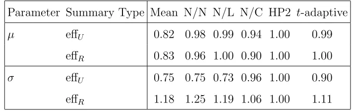
estima-tion. Eﬃciencies are deﬁned in the same way as before. The t-adaptive estimator does perform better than or as well as MEM-estimators with regard to location esti-mation. For scale estimation, it does not show overall better performance compared

to other ones.

Table 2.4: Estimated eﬃciencies of t-adaptive estimators relative to Huber’s Pro-posal 2

Parameter Summary Type Mean N/N N/L N/C HP2 t-adaptive

µ eﬀ_U 0.82 0.98 0.99 0.94 1.00 0.99

eﬀ_R 0.83 0.96 1.00 0.90 1.00 1.00

σ eﬀ_U 0.75 0.75 0.73 0.96 1.00 0.90

eﬀ_R 1.18 1.25 1.19 1.06 1.00 1.11

Summary type: eﬀ_U, usual; eﬀ_R, robust. Estimators: Mean, sample mean; N/N(L, C),

robust likelihood with normal (Laplace, Cauchy) contamination; HP2, Huber’s Proposal 2.

(45)

Figure 2.6: Boxplot of estimated degrees of freedom versus true degrees of freedom

for the t-adaptive estimators.

(46)

Chapter 3 Bayesian Inference for Robust

Error Contamination Models with

Application to Time Series Data

3.1 Introduction

There has been a rapid growth in the subject of robust estimation for time

se-ries models in the last two decades. The early proposals mostly dealt with auto-regressive processes. Denby and Martin (1979) proposed a generalized M-estimator (GM-estimator) by adding a bounded weight function in the M-estimation equation.

(47)

residual auto-covariances, were proposed by Bustos and Yohai (1986) as an

alterna-tive to the GM-estimator and K¨unsch’s method. However, these methods do not have satisfactory robustness properties for moving average or mixed auto-regressive mov-ing average (ARMA) models. Bustos and Yohai (1986) proposed estimators based on

truncated residual autocovariances, or TRA estimators, to overcome the deﬁciency. TRA estimators are qualitatively robust for stationary and invertible ARMA models, but have fairly low breakdown points. A diﬀerent method of dealing with additive

outliers in time series models, based on recursive generalized M-estimator, was intro-duced in Allende and Heiler (1992), and was shown to outperform other previously proposed methods in a Monte Carlo study. But the method suﬀers from the problem

of costly computation and the lack of theoretical robustness results. More recently, de Luna and Genton (2001) proposed robust, simulation-based estimation of ARMA models inspired by the indirect inference method.

In this chapter we present an alternative robust approach for ARMA models contaminated by additive outliers, which is based on the robust error contamination

model described in Chapter 2, and implemented through Bayesian inference. We call this new robust estimator BMEM-estimator.

The chapter is arranged as follows. In Section 2 we describe the error contami-nation model and the theoretical robustness properties, and in Section 3 we present

(48)

3.2 Robust Error Contamination Models with

Ap-plication to Correlated Data

In this chapter, we will restrict out attention to the invariant error model

W_i =X_i+τ σZ_i, i= 1, . . . , n. (3.1)

WithX₁, . . . , X_n having joint density f(x;θ), the joint density ofW₁, . . . , W_n is

f_W(w|θ, , τ) =

· · ·

f(w₁−τ σz₁, . . . , w_n−τ σz_n;θ)

n

i=1

G(dz_i), (3.2)

where

G(z) = (1−)I(0≤z) +

_z

−∞

g(x)dx.

3.2.1 Application to Correlated Data

The theoretical robustness results derived for independent and identically distrib-uted data in Chapter 2 can be directly extended to the case where X₁, . . . , X_n are correlated. Deﬁne

a_n(u;θ) = n

· · ·

f(s;θ)

n

i=1

1

τ σg

u_i−s_i τ σ

ds_i

,

and

(49)

where h(u;θ) is the contaminated density under the error model (3.1). With these

deﬁnitions, the likelihood score function becomes

ψ(u;θ, , τ) = ∂

∂θlnh(u;θ)

= q˙(u;θ) + ˙an(u;θ)

q(u;θ) +a_n(u;θ),

where ˙q(u;θ) = (∂/∂θ)q(u;θ) and ˙a_n(u;θ) = (∂/∂θ)a_n(u;θ). Deﬁne

p_n(u) = 1

τ σ n i=1 g _u i τ σ , and write

ψ(u;θ, , τ) = q˙(u;θ)/pn(u) + ˙an(u;θ)/pn(u)

q(u;θ)/p_n(u) +a_n(u;θ)/p_n(u). (3.3) In the appendix (A.9) we prove that iff is multivariate normal andg has polynomial-like tails or exponential-polynomial-like tails (see (2.9) and (2.10)), then

lim min|ui|→∞

q_p(_nu₍;_uθ₎)+q˙(u;θ)

p_n(u)

= 0. (3.4)

Therefore the behavior of the score function is determined by the tail behavior of

a_n(u;θ)/p_n(u) and ˙a_n(u;θ)/p_n(u). Note that

a_n(u;θ)

p_n(u) =

n _{· · ·} _f₍_s_;_θ₎n

i=1

g((u_i−s_i)/τ σ)

g(u_i/τ σ) dsi

.

and

˙

a_n(u;θ)

p_n(u) =

(∂/∂θ)a_n(u;θ)

p_n(u) .

(50)

For the case of polynomial-like tails, note that lim_|_u_|→∞g(u+b)/g(u) = 1 and

that limits and integration are interchangeable, so

lim min|ui|→∞

· · ·

f(s;θ)

n

i=1

g((u_i−s_i)/τ σ)

=

· · ·

f(s;θ)

n

i=1

lim |ui|→∞

g((u_i−s_i)/τ σ)

=

· · ·

f(s;θ)

n

i=1

1ds_i

= 1. (3.5)

Equations (3.3), (3.4) and (3.5) lead to

lim min|ui|→∞

ψ_θ

(σ)(u;θ, , τ)

= lim

min|ui|→∞

∂ ∂θ₍_σ₎

· · ·

f(s;θ)

n

i=1

g((u_i−s_i)/τ σ)

,

where θ₍_σ₎ denotes all parameters except σ. Since the gross errors in the invariant error model (3.1) includes σ, we need to treat the σ component of the score function diﬀerently, which is written as

lim min|ui|→∞

ψ_σ(u;θ, , τ)

= · · · (∂/∂σ)f(s;θ) _n

i=1{g((ui−si)/τ σ)/τ σ} dsi

_n

i=1g(ui/τ σ)/τ σ

. (3.6)

In light of (3.5) and the assumption that limits, integration and diﬀerentiation are interchangeable it follows that

lim min|ui|→∞

∂ ∂θ₍_σ₎

· · ·

f(s;θ)

n

i=1

g((u_i−s_i)/τ σ)

= ∂

∂θ₍_σ₎minlim|ui|→∞

· · ·

f(s;θ)

n

i=1

g((u_i−s_i)/τ σ)

(51)

Therefore

lim min|ui|→∞

ψ_θ

(σ)(u;θ, , τ) = 0.

The σ component of the score function is diﬀerent from other ones due to the fact

that the density of the added errors τ σZ₁, . . . , τ σZ_n depends on σ. In the appendix (A.10), we show that

lim min|ui|→∞

ψ_σ(u;θ, , τ) = n(p−1)

σ . (3.7)

where p is the power of the polynomial decreasing tails, i.e., g(u) ∼ u−p. So the

Cauchy error contamination model (p= 2) yields a redescending score function except for scale estimation, which is bounded by n/σ.

For the case of exponential-like tails, we allowg(u) to have diﬀerent tails asu→ ∞

and u→ −∞:

lim

u→∞

g(u+b)

g(u) = exp(c1b), u→−∞lim

g(u+b)

g(u) = exp(c2b),

for some constants c₁ and c₂. Set N₁ to be any subset ofN ={1, . . . , n}, and let N₂

be the set diﬀerence N −N₁. Then

lim

uk→ ∞, k∈N1

uj→ −∞, j∈N2

· · ·

f(s;θ)

n

i=1

g((u_i−s_i)/τ σ)

=

· · ·

f(s;θ)

k∈N1

lim

uk→∞

g((u_k−s_k)/τ σ)

g(u_k/τ σ)

j∈N2

lim

uj→−∞

g((u_j −s_j)/τ σ)

g(u_j/τ σ) ds

=

f(s;θ) exp

−c1 τ σ

k∈N1

s_k− c2 τ σ

j∈N2

s_j

ds. (3.8)

It follows that

lim

uk→ ∞, k∈N1

uj→ −∞, j∈N2

ψ_θ

(σ)(u;θ, , τ) = ∂

(52)

where v_k =−c₁/τ σ for k ∈N₁, v_j =−c₂/τ σ for j ∈N₂ and m_f(·,θ) is the moment generating function of f(·,θ), assumed to exist. So the error contamination model with the exponential-like tails results in a bounded score function except for σ. In Chapter 2 we showed that for the invariant error model with exponential-like tails,

the score function for σ is unbounded in the case of independent and identically distributed data. The proof in Appendix A.11 shows that it is unbounded in the case of correlated data as well.

3.2.2 Types of Outliers for Time Series Data

Let{X_t, t∈(1, . . . , n)}be a stationary stochastic process. An auto-regressive moving average (ARMA) time series of order (p, q) is deﬁned by

X_t−µ=

p

i=1

α_i(X_t₋_i−µ) +

q

j=1

β_je_t₋_j +e_t, (3.9)

where {e_t} is assumed to be independently and identically distributed with mean

zero and ﬁnite variance δ2, which is selected to make Var(X_t) = σ2 . When {e_t} is normal, {X_t} has a N(µ, σ2) distribution. We assume that model (3.9) is a causal and invertible process (Fuller 1996).

There are two types of outliers generally considered for time series data: innova-tion outliers (IO) and additive outliers (AO). The time series {X_t} is said to have

Robust Estimation via Measurement Error Modeling

Abstract

Biography

Acknowledgements

Contents

List of Figures

List of Tables

Chapter 1

Introduction and Overview

1.1

Motivation

1.2

Robust Statistics

1.3

Measurement Error Models

1.4

Robust Likelihood Approach via Measurement

Error Modeling

1.5

Research Overview

Chapter 2

Robust Estimation for

Location-Scale Models

2.1

Introduction

2.2

Robust Properties from Error-Contamination

Models

2.2.1

Influence Function Properties

2.2.2

Location-Scale Model Tuning Parameter

Determina-tion

2.2.3

t

-adaptive Error Contamination Models

2.3

Simulation Study

2.3.1

Performance for Small

B

2.3.2

Comparison with Huber’s Proposal 2

2.3.3

Adaptivity of the

t

-Adaptive Approach

Chapter 3

Bayesian Inference for Robust

Error Contamination Models with

Application to Time Series Data

3.1

Introduction

3.2

Robust Error Contamination Models with

Ap-plication to Correlated Data

3.2.1

Application to Correlated Data

3.2.2

Types of Outliers for Time Series Data