Ripple Droop Control: Control of Distributed Storage Devices with Droop Control using AC Voltage Injection.

(1)

ABSTRACT

FREGOSI, DANIEL JESSE. Ripple Droop Control: Control of Distributed Storage Devices with Droop Control using AC Voltage Injection. (Under the direction of Subhashish Bhattacharya.)

This work is concerned with the control of distributed devices on the power

distribu-tion system using a power-line signal injecdistribu-tion technique. We propose a method to control

power transfer in a plug-and-play manner from distributed energy storage devices such

as plug-in electric vehicles without the use of external communications. Ripple voltage

injection has been used to control distributed loads to implement demand response. We

propose a novel technique to improve ripple control by utilizing power-frequency droop on

the injected signal to control the power flow of distributed storage devices. Droop enables

an arbitrary number of distributed devices to communicate bi-directionally with a defined

response time to achieve power sharing. By controlling distributed storage through ripple

control, communication systems on the grid are freed to perform other functions. This

thesis is an effort to demonstrate the feasibility of the proposed method and to identify

(2)

(3)

Ripple Droop Control: Control of Distributed Storage Devices with Droop Control using AC Voltage Injection

by

Daniel Jesse Fregosi

A dissertation submitted to the Graduate Faculty of North Carolina State University

in partial fulfillment of the requirements for the degree of

Doctor of Philosophy

Electrical Engineering

Raleigh, North Carolina

2014

APPROVED BY:

Srdjan Lukic Mo-Yuen Chow

Xiangwu Zhang Subhashish Bhattacharya

(4)

DEDICATION

In this thesis and in all that I do, I strive to be a humble servant to God, from whom I

(5)

BIOGRAPHY

Danny Fregosi was raised in Harrisburg and then Concord North Carolina. He is the son

of Lorrie and Ronald and the younger brother of Josh. Danny graduated from Central

Cabarrus High School and got his Bachelor’s degree from NC State. He married his wife

Anna while in Graduate School. Upon finishing his degree, Danny will begin working for

(6)

ACKNOWLEDGEMENTS

I would like to thank the organizations who supported me during my graduate studies.

First I would like to thank the leaders in the ECE department at NC State and at

the FREEDM Systems Center for providing excellent opportunities for education and

research. I would like to thank the MIT Lincoln Laboratories and the US Department of

Defense for funding me through fellowships. Lastly, I would like to thank Sandia National

Laboratories for their generous student internship program.

I would like to thank all of those who mentored me during my time at NC State: my

advisor Dr. Subhashish Bhattacharya for his support, guidance, and his overall

enthusi-asm for research; Dr. Stan Atcitty for his professional, technical, and personal mentoring;

Dr. Leda Lunardi for her guidance, especially during the difficult first year of graduate

school; and the numerous other professors who put the effort into being excellent teachers.

Finally, I’d like to thank my family: Anna, Mom, Dad, Josh, Dianne, Mya, Tabb,

Tena, and Nathan, for their love and support. I’d like to thank my church families at

Hope and at Brooks. Finally I’d like to thank the friends I have made at FREEDM who

have helped me in my schoolwork and in providing a fun and interesting atmosphere to

work: Tom, Ryan, Phil, Ghazal, Mengqi, Edward, Saman, Babak, Behzad, Hesam, Lee,

(7)

LIST OF TABLES

Table 1.1 Value of Ancillary Services and Cost of Storage Technologies [14][15] 4

Table 3.1 IEEE 13 Bus Feeder Parameters . . . 27

Table 3.2 Comparison of Utility-Scale and Secondary-Use EV Energy Storage 28 Table 3.3 Common PHEV/EV Battery and Charger Sizes [2] . . . 30

Table 3.4 Bi-directional EV Charger Specifications . . . 31

Table 3.5 Ripple Droop Control Parameters . . . 32

Table 4.1 Feeder Impedance Matrix . . . 44

Table 5.1 Bi-directional EV Charger Specifications . . . 78

Table 5.2 Inverter Controller Compensator . . . 84

Table 6.1 RTDS Model Specifications - HIL Experiment . . . 103

Table 6.2 Typhoon Model Specifications . . . 107

Table 6.3 AIXControl Program Specifications . . . 108

(10)

LIST OF FIGURES

Figure 1.1 Balancing Requirement for NWPP for August Day [24] . . . 2

Figure 1.2 Balancing Requirement for NWPP for August Month [24] . . . 3

Figure 2.1 Power Flow Circuit . . . 13

Figure 2.2 Power Flow Phasor Diagram . . . 14

Figure 2.3 Power Sharing with Droop Control . . . 15

Figure 2.4 Power-Frequency Droop Closed Loop Block Diagram . . . 17

Figure 2.5 Reactive Power-Magnitude Droop Closed Loop Block Diagram . . 18

Figure 2.6 Reactive Power Sharing with Droop in Injected Signal . . . 20

Figure 2.7 Central Control and Distributed Storage on a Feeder . . . 21

Figure 2.8 Real Power Sharing with Droop in Injected Signal . . . 22

Figure 2.9 Closed Loop Block Diagram with Frequency as Input . . . 23

Figure 2.10 Central Inverter Closed Loop Block Diagram . . . 23

Figure 2.11 Adjustable offset droop slope . . . 24

Figure 3.1 IEEE 13 Bus Feeder . . . 26

Figure 3.2 IEEE 13 Bus Feeder with 500 EV Chargers . . . 29

Figure 3.3 Bi-directional EV Charger Schematic . . . 31

Figure 4.1 Simple Step Response with Feedback Delay . . . 35

Figure 4.2 Step Response of the System with Various Delay Magnitudes . . . 36

Figure 4.3 Arbitrary System with Multiple Voltage Sources and Loads . . . . 39

Figure 4.4 Eigenvalues of 32 Inverter System (m = 0.001 and k = 0.005) . . . 45

Figure 4.5 Simplified Droop Control Block Diagram . . . 45

Figure 4.6 Simplified Central Controller Block Diagram . . . 46

Figure 4.7 Eigenvalues of 32 Inverter System with Increasing m (top to bottom) 47 Figure 4.8 Eigenvalues of 32 Inverter System with Decreasing k (top to bottom) 48 Figure 4.9 Eigenvalues of System with Varying Number of EV . . . 49

Figure 5.1 Traditional Ripple Voltage with Series Line Filter . . . 51

Figure 5.2 Zero-sequence Ripple Voltage with Neutral Wire Filter . . . 52

Figure 5.3 Central Inverter Control for Zero-Sequence Signal Injection . . . . 53

Figure 5.4 Schematic for Control of Unbalanced EV Chargers with Ripple Droop 54 Figure 5.5 Results for Control of Unbalanced EV Chargers with Ripple Droop 55 Figure 5.6 Ideal Conservation of Power in Ripple Droop Control . . . 56

Figure 5.7 Division of Injected Power in Ripple Droop Control . . . 57

Figure 5.8 IEEE 13 Bus Feeder with One EV Charger per Phase per Bus . . 59

Figure 5.9 Leakage Power and Power Received vs Power Injected . . . 60

(11)

Figure 5.11 Power Received vs Power Injected as the System Load Varies . . . 62

Figure 5.12 Leakage Power vs Power Injected as the Number of EV Varies . . 63

Figure 5.13 Power Received vs Power Injected as the Number of EV Varies . . 63

Figure 5.14 Line Leakage Derivative versus Central Power under Varying Loads 66 Figure 5.15 Perturbation of Ripple Frequency to for Leakage Estimation . . . 67

Figure 5.16 Power Received versus Power Injected Actual and Estimated Values 68 Figure 5.17 Leakage Power versus Power Injected Actual and Estimated Values 69 Figure 5.18 Feeder Voltage Profile for Varying Frequencies . . . 71

Figure 5.19 Feeder Voltage Profile for Fundamental and Ripple Magnitudes . . 73

Figure 5.20 Maximum Angle vs Power Received as Load Varies . . . 74

Figure 5.21 Maximum Angle vs Power Received as Number of Chargers Vary 75 Figure 5.22 Signal Range versus Number of Distributed Chargers . . . 76

Figure 5.23 Inverse of Signal Range versus Number of Distributed Chargers . 77 Figure 5.24 Predicted Signal Range versus Number of Distributed Chargers . 77 Figure 5.25 EV Charger Schematic and Control Overview . . . 79

Figure 5.26 Superposition Ripple Droop Controller with Control Interactions . 81 Figure 5.27 Superposition Ripple Droop Controller with Filtered Feedback . . 81

Figure 5.28 Cascaded Ripple Droop Controller to Eliminate Control Interactions 83 Figure 5.29 Current Control Loop and Plant . . . 85

Figure 5.30 Fundamental Frequency Current Reference Generator . . . 87

Figure 5.31 Single Phase Power PLL . . . 87

Figure 5.32 Ripple Voltage Control Loop and Plant . . . 88

Figure 5.33 Single Phase to DQ Transformation . . . 90

Figure 5.34 DQ to Single Phase Transformation . . . 90

Figure 5.35 Ripple Frequency Droop Control Loop and Ripple Plant . . . 91

Figure 6.1 Overview of the Three Simulation Configurations . . . 95

Figure 6.2 Model of Grid-Connected Charger in PLECS . . . 96

Figure 6.3 Switching Simulation Results . . . 98

Figure 6.4 Output AC Voltage and Current of Switching Simulation . . . 99

Figure 6.5 Hardware-in-the-Loop Simulation Configuration . . . 101

Figure 6.6 Verification of IEEE 13 Bus Feeder Model in RSCAD . . . 104

Figure 6.7 Model of IEEE 13 Bus Feeder with 6 Chargers and an External Source in RSCAD. Breakout Views of Single Charger and its Con-troller . . . 105

Figure 6.8 Model of Charger in Typhoon HIL . . . 106

Figure 6.9 HIL Interface between Feeder and Charger . . . 107

Figure 6.10 Central Inverter PCC Voltages . . . 110

Figure 6.11 Central Inverter Current - Only Ripple Power . . . 110

Figure 6.12 Distributed Inverter Current - Ripple and Fundamental . . . 111

(12)

Figure 6.14 External Charger Current - Ripple and Fundamental . . . 112

Figure 6.15 External Charger Current - Smaller Time Scale . . . 113

Figure 6.16 External Charger Current - Smallest Time Scale . . . 113

Figure 6.17 Fundamental Current Step Response by Central Inverter . . . 114

Figure 6.18 Fundamental Current Step Response by Distributed Inverter . . . 115

Figure 6.19 Central Inverter Power at Initialization . . . 116

Figure 6.20 Central Inverter Ripple Voltage DQ Regulation at Initialization . 116 Figure 6.21 Distributed Charger Power at Initialization . . . 117

Figure 6.22 Response of Central Inverter to Initialization of Distributed Chargers118 Figure 6.23 Central Inverter Total Power Step Response 1 . . . 119

Figure 6.24 Central Inverter Total Power Step Response 2 . . . 119

Figure 6.25 Distributed Charger Ripple and Fundamental Power Step Response 1120 Figure 6.26 Distributed Charger Ripple and Fundamental Power Step Response 2120 Figure 6.27 Distributed Charger Current Step Response 1 . . . 121

Figure 6.28 Distributed Charger Current Step Response 2 . . . 121

Figure 6.29 External Charger Initialization PLL Frequency . . . 122

Figure 6.30 External Charger Initialization Ripple Voltage DQ Components . 123 Figure 6.31 External Charger Initialization Ripple Power . . . 123

Figure 6.32 External Charger Initialization Current . . . 124

Figure 6.33 Central Ripple Power during External Charger Initialization . . . 124

Figure 6.34 External Charger Ripple Power Step Response . . . 126

Figure 6.35 Distributed Chargers Ripple Power Step Response . . . 126

Figure 6.36 External Charger Current Step Response . . . 127

Figure 6.37 Distributed Charger Current Step Response . . . 127

Figure 6.38 External Charger Ripple Power - Disconnection from Grid . . . . 128

Figure 6.39 Distributed Charger Ripple Power - External Charger Disconnected 129 Figure 6.40 Central Charger Ripple Power - External Charger Disconnected . 129 Figure 6.41 External Charger Ripple Power - Re-connection to Grid . . . 130

Figure 6.42 Distributed Charger Ripple Power - External Charger Reconnected 130 Figure 6.43 Central Charger Ripple Power - External Charger Reconnected . . 131

Figure 6.44 Model of Feeder with 3 Central and 32 Distributed Chargers . . . 133

Figure 6.45 Model of Simplified Charger for System Simulation . . . 135

Figure 6.46 Central Inverter Ripple Power during System Initialization . . . . 136

Figure 6.47 Ripple Power of Distributed Inverters during System Initialization 137 Figure 6.48 Central Inverter Ripple Power System Step Response 1 . . . 139

Figure 6.49 Distributed Inverter Ripple Power System Step Response 1 . . . . 140

Figure 6.50 Central Inverter Ripple Power System Step Response 2 . . . 141

Figure 6.51 Distributed Inverter Ripple Power System Step Response 2 . . . . 142

(13)

(14)

Chapter 1 Introduction

1.1 Background

A major challenge to overcome for the widespread adoption of renewable energy sources

is their intermittency or non-dispatchable nature. In grids with high renewable energy

penetration, intermittency can lead to instability caused by generation load mismatch

[32], [30], [12].

The stability issue can be mitigated with the use of energy storage. Researchers at

the Pacific Northwest National Laboratory have examined the storage requirements for

accommodating an increase of renewable sources in the Northwest Power Pool [24], [29].

The researchers studied the impact of increasing the wind energy resource from 3.3 GW

to 14.4 GW. They found the total intra-hour balancing requirement for the power system

to be nearly 4 GW in both the generation increment and decrement directions to satisfy

a 99.5% probability that the storage will be sufficient to balance the system. To illustrate

the balancing requirement, the researchers simulated a typical balancing requirement

(15)

storage power needed to accommodate the wind power over one day and one month

respectively.

0 3 6 9 12 15 18 21 24

-2000 -1000 0 1000 2000 3000 4000

hours

MW

Figure 1.1: Balancing Requirement for NWPP for August Day [24]

Numerous studies have described the various benefits of adding storage to the utility

grid. A report from the U.S. Department of Energy defines various ancillary services for

the power grid [1]. Many of these services can be supplied by energy storage such as:

Regulation - minute by minute generation/load balance within a control area

Spinning Reserve - on-line generation capacity that can respond within 10 minutes

to compensate for generation or transmission outages

(16)

0 5 10 15 20 25 30 -6000

-4000 -2000 0 2000 4000 6000

days

MW

Figure 1.2: Balancing Requirement for NWPP for August Month [24]

Supplemental Reserve - off-line capacity that can respond within 10 minutes

Load Following - meeting hour-to-hour and daily load variations

Backup Supply - generation within an hour, for backing up reserves

There are many promising technologies for utility scale storage or bulk storage such

as batteries, flywheels, superconducting magnetic energy storage and compressed air [34].

Researchers at Sandia National Laboratories have studied the value for supplying such

services to the grid [14], [13], and have examined the costs associated with the various

forms of storage [15]. Results from their studies are summarized in Table 1.1. These

(17)

increase with increasing renewable energy penetration, storage becomes an even more

viable solution.

Table 1.1: Value of Ancillary Services and Cost of Storage Technologies [14][15]

Storage Application Life-cycle Estimated Benefit

Bulk Electricity Price Arbitrage $200 to $300/kW

Transmission Support $169/kW

Renewables Capacity Firming $192/kW

Storage Technology Energy Cost Power Cost

Lead-acid Batteries (VRLA) $200/kWh $225/kW

Lithium-Ion Batteries $500/kWh $175/kW

Sodium-Sulfur Batteries $250/kWh $150/kW

Compressed Air $120/kWh $600/kW

Low-speed Flywheel $380/kWh $280/kW

In addition, electric vehicles are expected to become much more widespread in the

coming years. Studies have been conducted on electric vehicles to show their impact on

the electric grid and how they can be used to support increased distributed generation

penetration [10], [36]. Using electric vehicle storage to provide grid support can be

eco-nomically beneficial to the owner since the grid support application adds value to the

storage which has already been purchased primarily for transportation. The downside

of this approach is the increased cycling of the battery which may lead to degradation.

Attempts must be made to study and understand the effects of increased cycling on the

battery to determine the proper value of using electric vehicle batteries for grid-support.

Researchers at the Pacific Northwest National Laboratory studied the feasibility of using

(18)

of wind power to the Northwest Power Pool [38]. They found that balancing requirements

can be met by utilizing the storage of 1.6 million electric vehicles that have at least a 33

mile range capacity battery if the vehicles are available for grid support while at home

and at work. The 1.6 million vehicles necessary is roughly 10% of the current number

of vehicles in the Northwest Power Pool. These results illustrate the large potential that

exists for electric vehicle storage to add grid support, given the projected outlook on

widespread electric vehicle adoption.

Researchers at Idaho National Laboratories have identified the need for

communi-cation between the charger and the electric grid so that the utility and consumer can

optimize the timing of charging and discharging [44]. Existing methods for controlling

distributed storage include the use of power line or wireless communication [16], [19].

These methods are capable of very high bandwidth allowing for flexibility and the use

of sophisticated protocols such as IEC 61850 [3]. These communication technologies are

effective for transferring large amounts of data and selectively communicating between

specific nodes in a system.

However, for control operations on the power system, the latency of the

commu-nication technology is of high importance. For wireless and power line commucommu-nication

technologies, the communication latency is a complex function of the protocol, scheduler,

amount of data, and number of nodes, routers and repeaters among other factors. In

ad-dition to controlling distributed storage, wireless or power line communication systems

may be expected to simultaneously perform high level operations such as advanced

me-tering infrastructure (AMI) functions, communication of real time pricing signals, remote

sensing, and phasor measurement unit (PMU) data acquisition.

(19)

found that with a scheduler designed specifically for smart-grid applications, certain

latency requirements for wide-area measurement systems (WAMS) [6] and automated

meter reading [22] can be met for a specific number of devices. However, the the additional

responsibility of performing control of distributed storage would be highly burden the

communication system.

1.2 Proposed Technique

We propose a method to control distributed devices by communicating through the power

line with an injected AC signal. The proposed method does not require additional

hard-ware as the electric vehicle charger is capable of generating the injected signal. The

method allows for plug-and-play of devices and the system latency does not increase as

the number of devices on the system increases. The injected signal is seen by all devices

and acts as a global variable, and the devices are controlled using droop control on the

injected signal.

This proposed method is called ripple droop control because it expands upon the

idea of ripple control by incorporating the basic elements of frequency-droop control.

Frequency droop control enables an arbitrary number of devices to communicate over

the power line with a fixed system response time. This is possible with frequency droop

because the system frequency acts as a global variable that can be accessed by each

device simultaneously and bi-directionally. Since the system frequency is analog, the data

transfer occurs continuously. In the ripple droop control application, the only constraint

for the system response or latency comes from the delay associated with filtering the

signal to isolate the targeted frequency and the delay associated with controlling the

(20)

communication hardware is needed since, due to the low frequency of the signal, the

power electronics in the electric vehicle chargers can be programmed to perform the

ripple voltage injection.

The objective of this work is to demonstrate the ability of the proposed ripple droop

control method to effectively control distributed storage devices on the power

distribu-tion system. The proposed method addresses the problem of coordinating distributed

devices on the power system without the use of additional communication equipment. If

a communication infrastructure exists on a feeder in which ripple droop control is

imple-mented, the communication system can be used as a backup in case of a failure in ripple

droop control.

For implementation of ripple droop control, the distributed devices must be able to

supply and absorb power on command and they must be controlled by a standard power

electronics inverter, capable of generating the ripple droop signal. The distributed devices

can be any combination of generation, load and storage.

The proposed method utilizes the inherent advantages of frequency droop control,

which include:

a global control variable (the frequency of the voltage signal). This is the frequency

of the fundamental voltage in traditional droop and the frequency of the injected

voltage in ripple droop. The frequency defines the system state and all devices on

the system have simultaneous read and write access to it.

power sharing in steady state according to droop slopes of the individual devices.

This is a result of the uniform frequency of the system in steady state.

(21)

The advantages of droop control are so beneficial that researchers have found

numer-ous applications for which droop can be used. Many of these applications are described

in the next chapter.

This work is the presentation of a previously unexplored application of droop control.

The contributions in this work include:

the use of frequency droop on injected signal in the distribution system.

the use of central inverter to control the frequency of the system by drawing and

supplying power to the injected signal. The central inverter is able to command a

specific quantity of power from the distributed inverters through a simple control

loop with a single integrator term.

performing single phase droop control on a three phase system at zero sequence.

The coordination is done by central inverter in order to generate only zero sequence

voltages which can be easily filtered to avoid upstream propagation.

a method to identify the number of distributed EV plugged in to the system and to

determine the amount of of power lost through the injected signal into loads. This

self commissioning process is necessary for the accuracy of the proposed method in

drawing a specific quantity of power from distributed sources.

a linearized state-space model of the ripple droop control system with distributed

inverters on the IEEE 13 Bus Test Feeder.

a three-stage cascaded controller to regulate fundamental frequency current and

output ripple voltage and frequency without undesired control interactions between

(22)

Lastly, the objectives targeted in this work are:

to explain a the derivation and basic operation of ripple droop control.

to describe a practical application for ripple droop control.

to present an accurate model of the system and analyze its stability

to discuss and address the limitations of the proposed method.

to demonstrate the method’s effectiveness through simulation and

hardware-in-the-loop experimentation

1.3 Organization

In the next chapter we describe the proposed method of ripple droop control. First, the

predecessor of ripple droop control, ripple control is presented. Next, we give an overview

of many of the previous uses of droop control. Our proposed method builds on the droop

control theory previously developed. In this chapter, we describe how to utilize frequency

droop on an injected signal to control distributed devices on the distribution system and

how a central device is able to coordinate the distributed devices.

In the following chapter, we describe the specifications for a particular application of

ripple droop control. We present specifications for the IEEE 13 bus distribution feeder

un-der consiun-deration, the capacity and power ratings for distributed EV batteries, schematics

for the EV chargers, and parameters for ripple droop control.

In the fourth chapter, we develop a state-space system model in order to understand

the dynamics of the system and to design the control. In this chapter, we analyze the

(23)

Next, we attempt to address limitations of the proposed method. We present an

analysis for the selection of the signal voltage, frequency, and power level. A detailed

analysis of the power lost due to loads (leakage power) on the system is presented. A

method for identifying the state of the system (amount of load and number of EV)

is presented as a solution to the leakage issue. To address the issue of signal spilling

into the transmission system, we propose zero-sequence signal injection in which the

central inverter coordinates droop on all three phases. The zero-sequence signal can be

easily filtered at the substation to avoid propagation of the signal into transmission.

Additionally, the power electronics hardware and control are described in detail in this

chapter.

Lastly, we attempt to validate the proposed method through simulation and

experi-mentation. The ripple droop control system on the distribution feeder is simulated with

average models for the power electronics components. Additionally, a switching-model

system is simulated with the feeder in a Real-Time-Digital-Simulator with an external

power electronics emulator and controller.

Future work includes testing the system on a variety of feeders and inclusion of more

(24)

Chapter 2 Ripple Droop Control

2.1 Review of Present Status

The ripple droop control method we propose adds droop control to the established method

of ripple control, thus enabling bi-directional communication and greater control function.

Before elaborating on our method, we briefly review the methods and applications of

ripple control and droop control.

Ripple Voltage Injection, also referred to as Ripple Control, is a commercially

avail-able, well-established technology used in power distribution systems for demand response

[33], [8]. Ripple control systems consist of a central generator that is controlled to inject a

voltage into the distribution grid at a specific, non-fundamental frequency. Specific relays

on the system are tuned to the ripple frequency and are programmed to connect or

dis-connect their loads from the grid whenever the ripple voltage is present. In this way, the

ripple control operator can control all participating loads from one location without the

use of additional communication equipment such as modems, dedicated lines, or wireless

(25)

nominal fundamental voltage and frequencies from 100-1000 Hz. Coding techniques have

been developed to enable more advanced control functions like tiered load shedding or

rate scheduling. Two of the main drawbacks and technical issues associated with ripple

control include:

limited capability and flexibility due to the uni-directionality of the signal

high ripple generator power requirement and introduction of harmonics into

trans-mission due to spill-over of the signal into the transtrans-mission system

Our proposed method improves upon traditional ripple control and directly addresses

these two drawbacks. We propose the use of frequency droop to enable all devices to

communicate simultaneously in a manner similar to the way frequency droop is used

in automatic generation control. To address the signal spill-over into transmission, we

propose to inject the ripple voltage at zero sequence (without phase offset) in all three

phases. The zero sequence voltage can more easily be filtered at the substation by a filter

on the neutral wire to avoid propagation into the transmission system.

A requirement for the proposed method is that the distributed devices must be active

and controlled by power electronics. The application we have focused on in this work is the

control of distributed electric vehicle chargers. The electric vehicle batteries are controlled

by the proposed method to provide support for the grid. With the proposed control, the

distributed batteries are aggregated, acting as a single large storage device capable of

rapidly responding to a power command. Specifications for the target application are

given in Chapter 3 of this work and the zero-sequence signal injection is expanded upon

in Chapter 5.

The advantages of the proposed method over traditional Ripple Control are enabled

(26)

controlling the power output of large generators connected to a power system. The main

features of droop control are the ability of generators to automatically adjust their

me-chanical power input to match the electrical load on a system and the ability of generators

to share the load proportionately without the use of external communications. The power

output of a generator when connected to an infinite bus through an inductive line, such

as in Figure 2.1, is given in Eq. 2.1.

Figure 2.1: Power Flow Circuit

P = EV

ωL sin(δ) (2.1)

When the system’s load varies, the current drawn through the inductor varies and the

angle of the generator with respect to the angel of the system changes. Figure 2.2 and

Eq. 2.2 illustrate the relationship between the voltage and current phasors.

˜

(27)

L

Figure 2.2: Power Flow Phasor Diagram

The power drawn from the generator initially comes from the energy stored in the

rotating inertia. The frequency of the generator’s rotor is proportional to the mechanical

power input from the turbine minus the electrical power drawn by the load, as in Eq. 2.3.

˙

ωgen =

Pm−Pe

Kinertia

(2.3)

As the electric load on the generator increases with the mechanical power constant, the

rotor frequency decreases. This causes the angle between the generator and the grid

to increase, further increasing the power drawn from the rotor. This positive feedback

cycle is broken as the droop controller senses the change in frequency and adjusts the

mechanical power input according to a predefined droop function such as Eq. 2.4, where

m is the droop coefficient.

P_m∗ =P0−m(ωgen−ω0) (2.4)

The mechanical power is adjusted dynamically until equilibrium is reached for the rotor

frequency. The frequency at which the rotor reaches equilibrium is found by rearranging

the terms in Eq. 2.4 and is given in Eq. 2.5.

ωgen =ω0−

Pm−P0

(28)

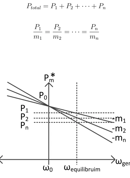
Using this simple control, a single generator and load will achieve generation-load balance.

In a system with multiple generators, when an equilibrium is reached, all generators

on the system be rotating at the same frequency and the system load will be shared

among generators proportional to their droop coefficients as in Eq. 2.6 and Eq. 2.7 [5].

A sample equilibrium from a 3-generator system is illustrated in Figure 2.3 where the

system frequency is ωequilibrium. This frequency acts as a global variable describing the

system’s state. The dynamics described in the single generator and load scenario are

present between all generators in a multi-generator system. For an equilibrium to be

reached, the frequency must be uniform in all generators, otherwise the relative angles

would not be constant in a steady-state.

Ptotal=P1 +P2 +· · ·+Pn (2.6)

P1

m1

= P2

m2

=· · ·= Pn

mn

(2.7)

0 0

1 m

gen 2 n

equilibruim 1

2 n

(29)

Researchers have expanded the application of droop control to islanded micro-grids

[17], [21], [18], parallel operation of uninterruptable power supplies (UPS) [7], and

dis-tributed active filters [9]. In the case of islanded micro-grids and parallel UPS, the

gen-eration in the system is often comprised entirely of inverters connected to batteries or

renewable energy sources rather than synchronous generators. When the load on an

in-verter varies, the inin-verter can supply the necessary power without any change in its

frequency, since the frequency is generated by the local controller and does not depend

on a rotating inertia. Therefore, to achieve the same power sharing in inverters in a

micro-grid as with traditional droop control in synchronous generators, a relationship

between power and inverter frequency is artificially implemented in control as in Eq. 2.8.

ω_inv∗ =ω0−m(Pinv−P0) (2.8)

Droop control in inverters is achieved by making the frequency a function of the electrical

power output, contrary to droop control in synchronous generators, where the mechanical

power is a function of the rotor frequency (Eq. 2.4). In both cases, the system frequency

reaches equilibrium and the power output from each source can be found according to

either Eq. 2.8 or Eq. 2.5. Figure 2.4 is shows the closed loop block diagram of the droop

controller along with the plant for an inverter controlled by droop. The frequency of the

system is represented as a disturbance input here. For a relatively a small angle (δ) the

dynamics are approximately linear and first order.

Further research has been done to study the stability of droop control in a micro-grid

[20], [27], and to find methods to improve the dynamic performance of droop control [23].

Researchers have used a variation of droop control for active filters to ensure that the

(30)

in-+_

P

0

P

m

ω

0

++

ω

system

+_

1 S

*

sin

E V

L





δ

ω

P

Figure 2.4: Power-Frequency Droop Closed Loop Block Diagram

crease, harmonic currents on the line increase and can be measured by the total harmonic

distortion (THD) of the line current. The active filters measure the THD and adjust their

conductance according to a predefined droop equation, Eq. 2.9.

G∗_af =G0−b(T HDmeasured−T HD0) (2.9)

The THD is seen by all active filters on the system, thus it is a global variable. The active

filters under the droop control will share the harmonic load proportional to their droop

coefficients. Another variation of droop control is a method of controlling the reactive

power output of inverters in a micro-grid [7]. The reactive power output of a source to

an infinite bus through and inductor, as in Figure 2.1 is given by Eq. 2.10.

Q= E

2

ωL − EV

ωL cos(δ) (2.10)

As a load’s reactive current varies, the voltage magnitudes (E and V) vary and the load

draws reactive power from the source. Under reactive power droop control, the source

(31)

droop control are shown in Figure 2.5.

E_inv∗ =E0−n(Qinv−Q0) (2.11)

+_

Q

0

Q

n

E

0

++

E

inv

Q

2

*

cos

E

E V

L









Figure 2.5: Reactive Power-Magnitude Droop Closed Loop Block Diagram

As the system reaches equilibrium, the reactive power is somewhat shared among

inverters. Reactive power sharing is not completely achieved because the voltage

mag-nitude is the variable used to control the reactive power and it is not uniform across

the system. A voltage gradient across the line is necessary for the transfer of reactive

power. Therefore, there is no global variable. Consequently, inverters closer to loads take

on more of the reactive power load than inverters separated by larger impedances due to

voltage drop across those impedances. In micro-grids, often line impedances have very

low inductances such that resistance of the lines has more of an impact on the power

transfer than the reactance. In this case, the real and reactive power equations given in

Eq. 2.1 and Eq. 2.10 are no longer valid. For low X/R ratios, the power flow

(32)

a function of phase angle. In these cases, researchers have proposed power-voltage and

reactive power-frequency droop [28], [25]. The steady-state error problem exists in this

case but for real power sharing. The power is not shared evenly since the voltage is not a

global variable. This problem was identified in [42] where an analogy was made between

traditional droop control in the main grid and power-voltage droop control in a

micro-grid. In this work, the authors suggest the global variable for power sharing should be

the DC voltage of each inverter. For this variable to be shared among all converters, the

authors suggest communication to be installed to transmit the information.

Lastly, researchers have addressed the problem of lacking a global variable in certain

cases when performing droop control and proposed a solution involving a signal injection.

These researchers studied a predominantly inductive micro-grid system for which

invert-ers share the real power, reactive power, and harmonic current [39], [40]. Here the sharing

of real power was accomplished through traditional power-frequency droop control.

How-ever, for the sharing of both reactive power and harmonic current, the researchers used

AC signals injected into the line at two alternate frequencies to represent the amount

of reactive power and harmonic current sourced by each inverter. The amount of power

transferred in each of these signals is proportional to the variable each one represents.

The researchers achieved uniform sharing of reactive power and harmonic currents by

de-coupling the variable used for communication from the quantity under control. In other

words, for real power sharing, the fundamental voltage frequency both communicates

the state of the system and controls power transfer. For reactive power sharing,

com-munication is achieved through the small injecting a signal, while the act of controlling

reactive power flow is achieved by altering the inverter fundamental voltage magnitude.

(33)

levels transferred at the alternate frequency can be used to control and represent other

quantities in the system. Figure 2.6 shows the closed loop block diagram for this reactive

power droop method.

Plant P-V Controller

Q-ωController Plant

+_ Q0 Pinjected m ωinjected_0 ++ ωinjected_system + 1 S * sin inv V E L   δ ωinjected Qinv + Pinjected_0 n V0

+₊ Vinv Qinv

2

* cos

inv inv

V V E

L L 

  

_ _

Figure 2.6: Reactive Power Sharing with Droop in Injected Signal

The researchers modified the traditional method, as shown in Figure 2.5, to include

frequency droop. The presence of the integrator in the power transfer plant ensures that

the frequency is uniform at steady state, therefore the quantity being controlled is shared

with no error.

2.2 Proposed Technique

The proposed method extends the droop concept by attempting to control distributed

de-vices in the power distribution system (rather than in a micro-grid) as in Figure 2.7. This

method differs from previous applications of droop for inverters because these inverters

are connected to a stiff grid, where local inverters in distribution cannot communicate by

altering the system frequency. Instead a signal is injected at a different frequency whose

scope is local. Power-frequency droop is performed on this superimposed signal, and a

small quantity of power is transferred among the inverters at the alternate frequency. The

(34)

constant to determine the desired power to be transferred from the distributed device at

fundamental frequency. In this way, the injected signal is used to coordinate and control

the distributed devices.

Figure 2.7: Central Control and Distributed Storage on a Feeder

Power sharing occurs at steady state because the injected signal frequency is uniform

across the system. The same closed loop dynamics that occur in droop control of inverters

in a micro-grid (Eq. 2.8 and Figure 2.4) apply to ripple droop control. The power

trans-ferred in the ripple signal is controlled in a closed loop manner, while the fundamental

power to be transferred is simply an output variable. This is illustrated in Figure 2.8.

An important distinction of ripple droop control from previous droop methods is the

ability to command a specific quantity of power rather than just reacting to changes in

the system (load, reactive load, harmonics, etc.). In other words, there is a controllable

input to the system. In ripple droop control, the input is received by the central inverter

from an external source. All distributed inverters react to the frequency of the injected

(35)

+_

P

ripple_0

_m

P

ripple

ω

ripple_0

++

ω

ripple_system

+_ 1

S

* sin

E V

L 



δ

ω

ripple

P

ripple

P

fund

/

P

ripple

P

fund

*

P

fund

LPF

Figure 2.8: Real Power Sharing with Droop in Injected Signal

Figure 2.8 shows the distributed controller’s function of adjusting its frequency in

re-sponse to the power drawn in the injected signal.Pripple0 is a constant control parameter

although it is placed where an input is commonly placed in a closed loop block diagram.

A rearrangement of this block diagram in Figure 2.9 places ωripple system as the input.

This illustrates how the power in the injected signal can be altered by changes in the

system frequency.

In ripple droop control the system frequency is set by the central controller, whereas

in traditional droop control the system frequency is set as a function of the load on the

system. The central controller is able to command a specific quantity of power (positive

or negative) from the injected signal by altering its frequency. The central inverter is

controlled according to Eq. 2.12. Its closed loop dynamics are shown in Figure 2.10.

(36)

+_

P

ripple_0

P

ripple

m

ω

ripple_0 -+

ω

ripple_system

1 S

*

E V

L



δ

ω

ripple

ω

ripple

++

Figure 2.9: Closed Loop Block Diagram with Frequency as Input

k P

ω0 +

ωsystem

+_ 1

S 2 ripple V L  δ ω P + +_ P* 1 S ωoffset

Figure 2.10: Central Inverter Closed Loop Block Diagram

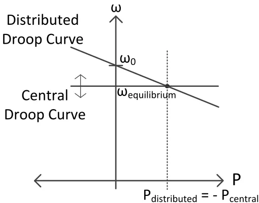
A plot of the droop curve of a distributed controller and that of the central controller

is illustrated in Figure 2.11. The central inverter frequency has been shifted downward

fromω0 such that its angle lags the distributed inverter’s angle. Consequently, the central

inverter draws power from the injected signal. The distributed inverter senses that power

is drawn and adjusts its frequency according to its droop slope until an equilibrium is

reached. In a system with multiple distributed inverters, the inverters share the power

drawn by the central inverter according to their droop slopes, as with traditional droop

control (Eq. 2.7).

(37)

ω

P

Distributed

Droop Curve

Central

Droop Curve

ω

equilibrium

P

distributed

= - P

central

ω

0

Figure 2.11: Adjustable offset droop slope

The distributed controllers have only a droop slope and the central controller has an

integrator coefficient. The integrator coefficient in the central controller determines the

damping of the system, while the droop slope constant determines the system response

time. A system model is developed and the dynamics and stability of the system are

analyzed in Chapter 4. In the following chapter, a specific application of ripple droop

control is described and system specifications are given for control of EV chargers on a

distribution feeder. In Chapter 6, various design considerations for ripple droop control

are investigated including filtering the signal from going upstream into transmission and

identifying and compensating for the signal power that is dissipated in loads on the

(38)

Chapter 3 Application Specifications

To illustrate the usefulness and practicality of the proposed ripple droop control method,

we have targeted the application of aggregating electric vehicle chargers on a distribution

system to provide frequency support to the grid. Frequency support is traditionally

pro-vided by fast-responding natural gas generators. However, energy storage and demand

response are becoming increasingly economical for this application [10]. As plug-in

elec-tric vehicles (EV) become more widespread, the storage capacity added to the grid will

be a valuable asset in providing stability and inertia [38].

Controlling distributed EVs for frequency support is an ideal application of ripple

droop control. EV chargers contain the necessary power electronics devices and controllers

to implement ripple droop control. The distributed storage on the feeder will respond

to the frequency of the injected signal. Through ripple droop control, the capacity of

the distributed storage is aggregated and controllable by a single central inverter. The

reference power command must be communicated to the central inverter by an outside

(39)

3.1 IEEE 13 Bus Feeder

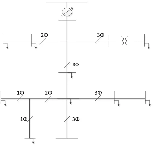
The IEEE 13 bus test feeder is used as the base system. All specifications for this feeder

are detailed in [37]. This feeder was selected as the base for our application because it

provides typical values for a distribution feeder. The feeder includes a variety of line sizes

and configurations as well as both balanced and unbalanced and both delta and wye

connected loads. A one-line diagram for the feeder is given in Figure 3.1.

1Φ

2Φ

3Φ

3Φ 3Φ

3Φ 2Φ

Figure 3.1: IEEE 13 Bus Feeder

Parameters for the feeder are shown in Table 3.1. The feeder has a neutral wire,

and, since the phases are not balanced, the neutral wire carries current under normal

conditions. The line impedances are given in the specification document in terms of self

(40)

Table 3.1: IEEE 13 Bus Feeder Parameters

Total Load 3.97 KVA p.f. 0.9

Line Voltage 4.16 kV (phase-phase rms)

Phase A 593.3 A p.f. 0.88

Phase B 435.6 A p.f. 0.93

Phase C 626.9 A p.f. 0.90

wire is included in the impedance values and it should be modeled as an ideal conductor.

The voltage regulator steps up the voltage to 1.0625 V, 1.05 V, and 1.06875 V per

unit on phases A, B, and C respectively. This is done so that all loads on the system

are subject to 1±0.05 V p.u. The generation and transmission system upstream of the

feeder is modeled as an infinite bus.

3.2 Electric Vehicle Storage

In this application, the distributed storage on the feeder that exists in the batteries of

plug-in electric vehicles can be aggregated to act as a single utility-scale energy storage

system. Utility-scale energy storage systems supply mega-watts of power to the grid and

can go from sourcing rated power to sinking rated power in less than a second [43], [4].

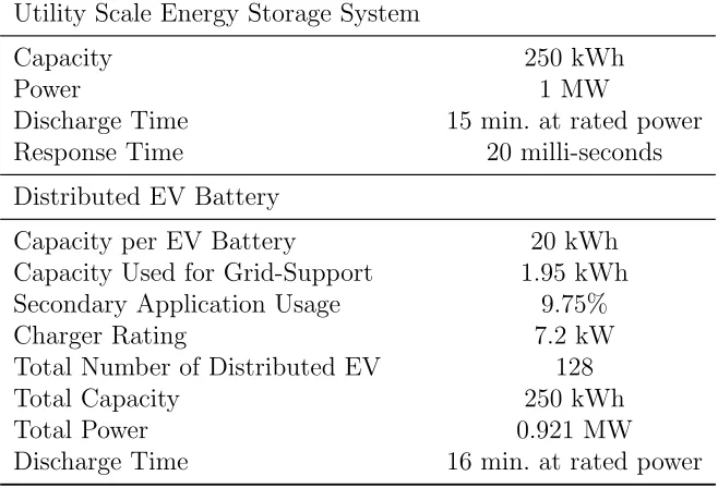
Typical values for such a system are given in the top section of Table 3.2.

The number of EV plugged into the feeder is taken to be 128 for this application.

The EV chargers were placed throughout the feeder, four on each bus on each phase,

according to Figure 3.2.

(41)

Table 3.2: Comparison of Utility-Scale and Secondary-Use EV Energy Storage

Utility Scale Energy Storage System

Capacity 250 kWh

Power 1 MW

Discharge Time 15 min. at rated power

Response Time 20 milli-seconds

Distributed EV Battery

Capacity per EV Battery 20 kWh

Capacity Used for Grid-Support 1.95 kWh

Secondary Application Usage 9.75%

Charger Rating 7.2 kW

Total Number of Distributed EV 128

Total Capacity 250 kWh

Total Power 0.921 MW

Discharge Time 16 min. at rated power

battery used for grid-support is a small fraction of the overall battery capacity (9.75%

in this application). The power rating for each EV is selected such that a single-phase

level 2 charger is easily capable of supplying it. The bottom half of Table 3.2 gives the

specifications for the individual EV battery and charger capacity and power rating. The

sum of the capacities and power ratings for the distributed chargers approximately equal

a single utility-scale energy storage system. To verify that the EV battery and charger

power ratings are practical, several common EV battery capacities and charger sizes for

level 2 chargers are given in Table 3.3 [2]. The proposed ripple droop control method

can be implemented for both single-phase and three-phase systems. We assume the EV

chargers are single-phase for this application because three-phase level-3 chargers not

economically practical for household use.

(42)

~

Central

Storage

~

~ ~

~

x12

_x12

x8

x12

x8

x4

x12

Figure 3.2: IEEE 13 Bus Feeder with 500 EV Chargers

communication technology such as the GE DuraStation ($4,500) and the Siemens Smart

Grid EVSE charger are significantly more expensive than basic chargers such as the

Schneider charger ($800). This illustrates the cost of communication equipment. To

im-plement ripple droop control, the chargers need no additional hardware. The chargers all

have a requisite micro-controller and current and voltage sensors necessary to perform

(43)

Table 3.3: Common PHEV/EV Battery and Charger Sizes [2]

Plug-in Hybrid Electric Vehicle (PHEV) Battery Capacity

Toyota Prius 4.4 kWh

Honda Accord 6.6 kWh

Volkswagen TwinDrive 12 kWh

Chevrolet Volt 16.5 kWh

Electric Vehicle (EV) Battery Capacity

Chevrolet Spark 20 kWh

Ford Focus Electric 23 kWh

Nissan Leaf 24 kWh

Mercedes BlueZero 35 kWh

Tesla Roadster 56 kWh

Level 2 Charger (240 V/1Φ) Power (Current)

GE, Schneider, Siemens 7.2 kW (30 A)

Ford 7.68 kW (32 A)

Eaton 16.8 kW (70 A)

3.3 Charger Specifications

The chargers considered in this application are off-board, bi-directional, conductive level

2 chargers. A comprehensive review of EV chargers is given in [45], and bi-directional

chargers are examined specifically in [11]. The charger considered is a two-stage converter.

The AC-DC stage is a single-phase half-bridge configuration. This stage converts the 240

V AC voltage to 400 V at DC. The DC-DC stage is chosen to be a bi-directional buck

converter. This topology is chosen for its simplicity. If isolation is required, a dual active

bridge topology could be selected instead. The DC-DC stage converts the 400 V DC bus

voltage to the battery voltage of 300 V. For our control method, the AC-DC stage controls

(44)

the AC-DC stage regulates the DC bus voltage. The battery and dc-dc converter are later

modeled as an ideal DC source, while they are shown here for completeness. A detailed

description of the power electronics control is given in chapter 5. The overall charger

schematic and list of parameters, including the distribution transformer, are given in

Figure 3.3 and in Table 3.4.

Table 3.4: Bi-directional EV Charger Specifications

EV Charger

Transformer Ratio 2.4 kV:240 V

Transformer Z 0.02 + j0.03 p.u.(50 kVA, 60 Hz)

Lleakage 91.7 µH (secondary)

AC Voltage 240 Vrms

Switching Frequency 10 kHz

Lac 2.2 mH

Cac 20 µF

Vdc bus 400 V

Vdc_bus

Lac

Vdist

2.4 kV: 240 V Distribution Transformer

Cdc_bus

Vbattery

Lbuck

AC-DC H-Bridge

DC-DC Bi-directional Buck

Lleakage

Cac

(45)

3.4 Ripple Droop Control Parameters

As mentioned in the previous section, for the target application 128 distributed EV

chargers and batteries are added to the IEEE 13 bus feeder to constitute an aggregate

capacity of 250 kWh and power of nearly 1 MW. In this section, the remaining parameters

for the system and its control are presented. The design and selection criteria for several

of the parameters presented here are explained in next couple chapters. The purpose of

this section is to present the information concisely in a single location. The parameters

are given in Table 3.5.

Table 3.5: Ripple Droop Control Parameters

Injected Signal

Voltage Magnitude 3%

Frequency 90 Hz

Signal Range (Central Inverter) 3.46 kW

Power per Charger (Distributed Inverter) 27 W

Fundamental Power/Signal Power Ratio 267

Response Time 2.5 seconds

Droop Slope 0.00343 radians/s/W

The injected signal voltage magnitude is selected to be 3% of the nominal voltage,

which complies with the harmonic voltage standard’s recommendation of 3% for

indi-vidual voltage harmonics [31]. The frequency selection and power range that the central

inverter can pull from or put into the injected signal are a function of the line and filter

impedance, injected signal voltage, and amount of load on the system and are derived

(46)

The response time is related to the speed of the controller, including the extraction

filter that separates the injection signal measurements from the fundamental frequency

signal and its harmonics. It is shown that the droop slopes can be set to achieve an

arbitrarily fast system response, however the response time for filtering the injected

signal from the line is the limiting factor. Due to the delay associated with the filtering,

the system response time is limited. The central integrator gain term controls damping

(47)

Chapter 4 System Model

The purpose of this chapter is to model and analyze the system dynamics. By describing

the system in terms of a mathematical model, we are able to quantitatively examine the

stability and performance of the system. In addition, with the model we are able properly

select values for the droop slope and the central inverter integrator gain term. Lastly, we

examine the effects of of changing the number of distributed chargers on the system.

4.1 Model Development

In the development of the system model, a few approximations are made for simplicity

and linearization. For each of the four approximations (ideal power measurement, time

invariant system, inductive line, small angle), a justification is given.

Approximation 1: Ideal Power Measurement.The first approximation is that we have an ideal measurement of the magnitudes of the injected signal voltage and

current. The power in the injected signal is an input to the droop controller. Ideal

(48)

injected signal. Therefore, this approximation states that only power in the ripple signal

is included and fundamental frequency components can be ignored. Furthermore, ideal

measurement means there is no delay from changes in the actual magnitude and changes

in the measured magnitude. In the extraction filter design section in the next chapter,

the rejection capability and the speed of the extraction filter are examined. The speed

of the filter does not have a significant effect on the dynamics of ripple droop control

system if its speed is at least an order of magnitude faster than the system speed. The

simple example in Figure 4.1 and Figure 4.2 illustrates a feedback loop with a delay in

the feedback path.

+_

input

S



output

1

delay

S

 

(49)

Figure 4.2: Step Response of the System with Various Delay Magnitudes

The step response of the system for delays of different values (fractions of the system

time constant, τ) are shown. The results show that the diminishing effect of the delay

as its time constant becomes a small fraction of the overall time constant. In the ripple

droop control system, for this approximation to be accurate, the speed of the system

(magnitudes of the dominant eigenvalues) should be at least an order of magnitude less

than the speed of the extraction filter.

Approximation 2: System Time Invariance.The second approximation is that the system parameters in the model remain constant. The two cases in which the system

model changes under normal operation is in the line reactance value and in the number

and location of EV on the feeder. The line reactance seen by the injected signal is a

function of the frequency of the injected signal. This approximation is accurate as long

as the variations in the signal frequency are small. The system frequency varies less than

1 Hz under nominal conditions.

(50)

not valid. The system model changes significantly as the number and location of EV on

the system changes. We desire to design a system which can accommodate the addition

and removal of EV’s. Therefore, we generate several models of the system under varying

numbers of EV chargers in this chapter.

To describe the system, we first develop a nonlinear state-space model, then linearize

the model. The states of the system are the angles of the chargers,δ1, δ2, . . . , δn. We will

use the central inverter angle as the reference angle. The quantities of the central inverter

have the subscript c in the notation. For a system with n total distributed chargers and

one central inverter, there are n+1 states. The central inverter angle is not a state (since

it is the reference), however, there is an integrator in the controller of the central inverter

which adds a state to the system. This integrator which is used to adjust the central

inverter frequency in order to meet the commanded reference power. The next-state

equations are given in Eq. 4.1. In the following equations, Px is the power supplied by

charger x, P∗ is reference power command, and K is gain in central inverter controller.

            ˙ δ1 ˙ δ2 .. . ˙ δn ˙

ωc of f set             =            

ω1−ωc

ω2−ωc

.. .

ω2−ωc

K(P∗−Pc)             (4.1)

The frequencies of each charger, ω1, ω2, . . . , ωn, ωc, are determined by the droop

con-trollers in each charger. The central inverter frequency is the nominal frequency plus the

offset term. These equation are shown in Eq. 4.2, where m is the droop slope and ω0 is

(51)

            ω1 ω2 .. . ωn ωc             =            

ω0−mP1

ω0−mP2

.. .

ω0−mPn

ω0+ωc of f set             (4.2)

The power supplied by each charger (Px) can be computed as a function of the state

variables, system parameters, and inputs to the system. Its computation is derived in the

next several equations. The power supplied by an AC source is given in phasor notation

in Eq. 4.3.

Pi =real[Ve_iIe_i∗] (4.3)

The voltage magnitude is a constant parameter and its angle is a state variable,

thus the voltage phasor can be computed simply. However, to find the current phasor,

Kirchoff’s Voltage Law must be used. For an arbitrary system with ground-connected

voltage sources and loads, as in Figure 4.3 where all possible paths from the source to

ground are shown, the current from any inverter, i, can be found by summing the currents

along all paths as in Eq. 4.4. In this equation,Zij is the total impedance between voltage

sourceiandj, andZload i is the equivalent impedance from the voltage sourceito ground

through all loads on the system.

e

Ii = e

Vi−Ve1

Zi1

+ Vei−Ve2

Zi2

+. . .+ Vei−Ven

Zin

+ Vei−Vec

Zic

+ Vei

Zload i

(4.4)

Using Eq. 4.3 and Eq. 4.4, the power from voltage source i to source j due to the current

(52)

V1

Vn

...

V2 Vc

load Vi

load

Figure 4.3: Arbitrary System with Multiple Voltage Sources and Loads

magnitude for all voltage sources.

Pij =real[|V|(cosδi+jsinδi)

|V|(cosδi−jsinδi)− |V|(cosδj−jsinδj)

Zij

] (4.5)

Multiplying the terms through gives Eq. 4.6.

Pij =rea[ V2

(

cos2_δ

i + sin2δi+ cosδicosδj+ sinδisinδj

Zij

+j(sinδicosδj −cosδisinδj)

Zij

)] (4.6)

Lastly, using the trigonometric identities (cos2_δ_+sin2_δ _{= 1) and (sin}_δ

(53)

sin(δi−δ1)), the equation can be simplified to Eq. 4.7

Pij =real[ V2

1 + cosδicosδj + sinδisinδj +jsin(δi−δj)

Zij

] (4.7)

Approximation 3: Purely Reactive Line Impedance. Given that the impedance between any two sources is purely reactive, the power transfer equation simplifies to the

easily recognizable form of Eq. 4.8. The approximate total power from inverter i is given

in Eq. 4.9.

Pij = V2

sin(δi−δj)

Xij

(4.8)

Pi = V2

(

sin(δi−δ1)

Xi1

+ sin(δi−δ2)

Xi2

+. . .+sin(δi−δn)

Xin

+sinδi

Xic

+ 1

Rload i

) (4.9)

For this application, the approximation that the line impedance is purely reactive is

fairly accurate. The impedance between two sources in the system is made up of the

transformer impedance and the line impedance. The equivalent low voltage impedance

for the line impedance is found by dividing by the square of the transformer turns ratio

(10 in this case). For this system, the transformer impedance is 23 mΩ + 92 µH and

the typical line impedance low voltage equivalent is 1.73 mΩ + 13.5 µH. At the selected

injection frequency of 90 Hz, the typical total reactance between chargers is about 118

mΩ and the total resistance is about 25 mΩ.

The impedances between all of the distributed chargers on the system are found

through simulation in the next section. With the impedance values, the voltage

magni-tude, and control parameters (m and K), all of the information is known for the next-state

equations. The final step in the development of the model is to linearize the equations

for the state variables (δ1, δ2, . . . , δn).

(54)

necessary for the linearization of the system. Eq. 4.8 is non-linear with respect to the

state variables, δ. A common solution is to approximate the sinusoidal function as in

Eq. 4.10. This approximation is accurate for low values of δ1−δ2. In the next chapter,

we define and determine the proper range of operation of the system such that all of the

angles of the distributed chargers are within 60◦ of the central inverter angle. With this

approximation, the power transfer equation reduces to Eq. 4.11.

sin(δ1−δ2)≈(δ1−δ2) (4.10)

Pi = V2

(

δi −δ1

Xi1

+ δi−δ2

Xi2

+. . .+ δi−δn

Xin

+ δi

Xic

+ 1

Rload i

) (4.11)

Collecting the equations and arranging them in matrix form gives the linearized

next-state equations in Eq. 4.12, whereCij =|V2|/Xij. In these equations, the system load is a

disturbance input and the power reference command is the control input. In the following

section, we will use the state-model to analyze the stability and dynamic performance of

(55)

            ˙ δ1 ˙ δ2 .. . ˙ δn ˙

ωc of f set             =                −mP i6=1

C1i mC12 . . . mC1n −1

mC21 −m

P

i6=2

C2i . . . mC2n −1

..

. ... . .. ... ...

mCn1 mCn2 . . . −mP

i6=n

Cni −1

KCc1 KCc2 . . . KCcn 0                            δ1 δ2 .. . δn

ωc of f set             +            

|V2_|_/R

load1

|V2_|_/R

load2

.. .

|V2_|_/R

load n 0             +             0 0 .. . 0 K            

P∗ (4.12)

4.2 Stability and Performance Analysis

The system stability depends on the eigenvalues of the state transition matrix. If all

eigenvalues of the state transition matrix are negative and the approximations are valid,

the system is asymptotically stable. In an asymptotically stable system, the system will

always return to an equilibrium unless one of the inputs causes an approximation to

become invalid. One of our approximations can become invalid if the system changes

configuration significantly or if the load power or the power reference command causes

the small angle approximation to become invalid. If an angle in the system goes above

90◦ then the system becomes unstable altogether.

In this system, the states are the angles of the distributed chargers relative to the

Ripple Droop Control: Control of Distributed Storage Devices with Droop Control using AC Voltage Injection.

ABSTRACT

DEDICATION

BIOGRAPHY

ACKNOWLEDGEMENTS

TABLE OF CONTENTS

LIST OF TABLES

LIST OF FIGURES

Chapter 1

Introduction

1.1

Background

1.2

Proposed Technique

1.3

Organization

Chapter 2