ABSTRACT
PUCKETT, PAIGE ROLLINS. The Rock Cross Vane: A Comprehensive Study of an In-Stream Structure. (Under the direction of Gregory D. Jennings.)
The rock cross vane, an in-stream boulder structure, consists of a U-shaped weir with the apex upstream at bed elevation and upward sloping arms that tie into downstream banks. The structure provides grade control, bank protection and scour pool development via a protected drop and arms that turn flow away from the banks. A physical model was used to measure the velocity distribution changes caused by a range of geometric configurations of the structure. Results showed linear and
THE ROCK CROSS VANE:
A COMPREHENSIVE STUDY OF AN IN-STREAM STRUCTURE
by
PAIGE ROLLINS PUCKETT
A dissertation submitted to the Graduate Faculty of North Carolina State University
in partial fulfillment of the requirements for the Degree of
Doctor of Philosophy
BIOLOGICAL AND AGRICULTURAL ENGINEERING
Raleigh, North Carolina 2007
APPROVED BY:
Dr. Gregory D. Jennings Chair of Advisory Committee
Dedication
For Joe.
What has been will be again, what has been done will be done again; there is nothing new under the sun.
Biography
Acknowledgements
This research was funded by the National Science Foundation Graduate Research Fellowship program and Department of Biological and Agricultural Engineering at North Carolina State University.
I would also like to recognize:
Joe Puckett, Greg Jennings, Mike Boyette, Garry Grabow, Jim Gregory, John
Table of Contents
List of Tables... vii
List of Figures ... x
Chapter 1:
History of the use of hydraulic structures related to the rock cross vane ... 1 Literature Cited ... 21
Chapter 2:
Effects of Rock Cross Vane Geometry on Velocity Distribution ... 24 Literature Cited ... 64
Chapter 3:
Rock Cross Vane Rapid Assessment Tool and Failure Guidebook ... 65 Literature Cited ... 107
Chapter 4:
Occurrence, Probability and Risk of Rock Cross Vane Failures in North
Carolina Stream Restoration Projects ... 108 Literature Cited ... 169
Chapter 5:
Restoration and Cross Vane Impacts on Benthos... 170 Literature Cited ... 190
Chapter 6:
Literature Cited ... 202
Appendix A:
Tables and Figures ... 204 Appendix B
List of Figures
Chapter 1
Figure 1.1 Profile View of Cross Vane Arm... 2
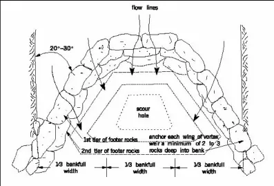
Figure 1.2 Plan View of Rock Cross Vane ... 3
Figure 1.3 Salmon weir at Quamichan Village on the Cowichan River, Vancouver Island... 5
Figure 1.4 Stone Fish Weir on Menai Strait ... 6
Figure 1.5 Chester Weir on the Dee River ... 10
Figure 1.6 Plan View of Rock Vortex Weir ... 12
Figure 1.7 Plan View of Rootwad Revetment... 13
Figure 1.8 Bendway Weir Theory ... 14
Figure 1.9 Installation of Concrete Iowa Vanes at Low Flow ... 16
Figure 1.10 Plan View of Rock Vane and J-Hook ... 17
Figure 1.11 Plan Views of Three Types of Long Crested Weirs ... 17
Figure 1.12 Formation of a Waterfall ... 19
Chapter 2 Figure 2.1 Plan View of the Velocity Distributions at Rock Cross Vane... 28
Figure 2.2 Diagram of a Step in a Channel ... 29
Figure 2.3 Hydraulic Jump... 31
Figure 2.4 Length of Jump for a Rectangular Channel ... 32
Figure 2.5 Site Layout ... 34
Figure 2.6 Observed Stage vs. Time of Storage Pond Drawdown ... 36
Figure 2.7 Plan View of Test Flume ... 38
Figure 2.8 Profile View of Rock Cross Vane Model ... 40
Figure 2.9 Profile View of Flume Stilling Basin and Baffle Outlet – Baffle Combination ... 41
Figure 2.10 Baffle Oulet – Baffle Combination ... 41
Figure 2.11 Test Run with the Pygmy Meter and AquaCount Calculator... 42
Figure 2.12 Flume test of drop ratio = 1, angle = 20˚, slope = 3% ... 43
Figure 2.13 Predicted and Actual Velocity Ratio for Drop, Angle, and Slope for Cross Section C... 50
Figure 2.15 Predicted Velocity Ratio versus Drop Ratio and Arm Slope for Cross Section C... 52
Figure 2.16 Residuals at Cross Section A... 53
Figure 2.17 Residuals at Cross Section B... 54
Figure 2.18 Residuals at Cross Section C ... 55
Chapter 3 Figure 3.1 Arm Washout... 76
Figure 3.2 Cross vane with a portion of the sill shifted or missing ... 77
Figure 3.3 Head cut at rock cross vane looking downstream ... 78
Figure 3.4 Bank erosion at cross vane leading to side cutting and headcut ... 80
Figure 3.5 Flow Expansion with Downstream Erosion ... 81
Figure 3.6 Shallow Pool with Vegetation... 82
Figure 3.7 Diagram of Drag and Lift ... 84
Figure 3.8 Constricted Rock Cross Vane ... 86
Figure 3.9 Piping caused by boulder spacing and poor backfill ... 87
Figure 3.10 Cross vane with improper alignment... 91
Figure 3.11 Cross vane backed into a pool... 91
Figure 3.12 Undersized Cross Vane in Bend ... 92
Figure 3.13 Vane on Bedrock... 93
Figure 3.14 Downstream scour from short steep arms ... 94
Figure 3.15 Steep Arm on Right Bank... 95
Figure 3.16 Cross vane sill installed too high... 96
Figure 3.17 Sill and backfill shifted downstream to pool ... 97
Figure 3.18 Poor Boulder Spacing ... 97
Figure 3.19 Boulders placed in pool to protect drop... 98
Figure 3.20 Undersized Boulders ... 99
Figure 3.21 Lack of vegetative bank protection... 100
Figure 3.22 Evidence of piping caused by insufficient backfill ... 101
Figure 3.23 Undercut Banks at Arms from insufficient footers... 101
Figure 3.24 Oversized rock cross vane ... 102
Figure 3.25 Bank erosion and head cut caused by an undersized vane ... 103
Chapter 4 Figure 4.1 Boulder of a Cross Sill in Assumed Conditions... 115
Figure 4.2 Free Body Diagram of Assumed Cross Sill Conditions... 115
Figure 4.4 Cross Sill with Head cut ... 117
Figure 4.5 Free Body Diagram of Cross Sill with Head cut ... 117
Figure 4.6 Cross Still Prime Conditions for Tipping... 118
Figure 4.7 Free Body Diagram for Tipping Conditions ... 118
Figure 4.8 Projects by County ... 125
Figure 4.9 Example Fault Tree for Sill Washout... 132
Appendix A Figure A-1 Profile View of Cross Vane Arm ... 206
List of Tables
Chapter 1
Table 1.1 Citations of Fish Weirs and Related Structures in North Carolina ... 7
Chapter 2 Table 2.1 Pipe Elevation, Length, and Slope ... 35
Table 2.2 Time Discharge Calculation ... 35
Table 2.3 Predicted Normal Depth and Observed Depth... 39
Table 2.4 Velocity Ratio for Three Test Runs at each Cross Section ... 44
Table 2.5 Factor Levels and Values ... 45
Table 2.6 Velocity Ratio for Cross Section by Test Run ... 48
Table 7 LSMEANS for Class Effects of Cross Section... 49
Table 2.8 Analysis of Variance for Response Surface Regression Model at Cross Section A... 53
Table 2.9 Analysis of Variance for Response Surface Regression Model at Cross Section B... 54
Table 2.10 Analysis of Variance for Response Surface Regression Model at Cross Section C ... 55
Table 2.11 SAS output for Parameters of Response surface Regression Model at Cross Section C... 56
Table 2.12 Flow Regime Calculations for Cross Section ... 58
Table 2.13 Area Ratio at Critical Depth and Brink Depth for 7.2 cfs ... 60
Chapter 3 Table 3.1 Rock Cross Vane Rapid Assessment Tool ... 74
Table 3.2 Failures and Major Indicators ... 75
Table 3.3 Types of Side cutting ... 88
Table 3.4 Potential Failure Paths ... 103
Chapter 4 Table 4.1 Failure and Major Indicators ... 122
Table 4.2 Projects and Site Data... 124
Table 4.4 Median rating of failure indicators by project... 135
Table 4.5 Frequency of Failure Indicators ... 136
Table 4.6 Frequency of Primary Causes of Failure... 138
Table 4.7 Frequency of Secondary Causes of Failure ... 139
Table 4.8 Occurrences of Failure Paths ... 141
Table 4.9 Correlation of Project Variable ... 143
Table 4.10 Effects of Project Variables on F1: Arm Washout ... 145
Table 4.11 Effects of Project Variables on F2: Sill Washout... 146
Table 4.12 Effects of Project Variables on F3: Head Cut... 147
Table 4.13 Effects of Project Variables on F4: Bank Erosion at the Structure... 148
Table 4.14 Effects of Project Variables on F5: Downstream Bank Erosion ... 149
Table 4.15 Effects of Project Variables on F6: Insufficient Scour Pool Development... 150
Table 4.16 Class Effects of Project on F1: Arm Washout ... 151
Table 4.17 Class Effects of Project on F2: Sill Washout ... 152
Table 4.18 Class Effects of Project on F3: Head Cut... 153
Table 4.19 Class Effects of Project on F4: Bank Erosion at the Structure... 154
Table 4.20 Class Effects of Project on F5: Bank Erosion Downstream of Structure ... 155
Table 4.21 Class Effects of Project on F6: Lack of Scour Pool Development ... 156
Table 4.22 Partial Correlation Matrix for Failure Indicators ... 157
Table 4.23 Failure Modes... 160
Table 4.24 Consequence Categories ... 162
Table 4.25 Detection Rating ... 163
Table 4.26 FMEA of a Rock Cross Vane, General Stream Restoration Usage... 164
Chapter 5 Table 5.1 Summary of Effects on Benthic Macroinvertebrates ... 176
Table 5.2 Restoration Priority Levels... 185
Appendix A Table A-1 Fractional Factorial Design Test Points ... 205
Table A-2 Velocity (ft/s) at Given Point for Test Run... 206
Table A-3 Velocity Ratio for Cross Section by Test Run... 210
Chapter 1:
Introduction
The rock cross vane is a structure used to maintain stream grade and to turn flow away from banks. It also provides a drop structure that creates a downstream pool for habitat and allows for a drop in bed elevation thereby allowing energy dissipation and lower bed slopes upstream and downstream where sinuosity is restricted. It is unique in that it acts as a weir, vane, and drop structure all in one. The upward sloping arms of the rock vane are similar to those of single arm vanes used to protect the outer stream bank of a curve where velocities increase. Figures 1.1 and 1.2 are profile and plan views of the rock cross vane.
Figure 1.2 Plan View of Rock Cross Vane Source: Rosgen 2001
If the current solution in stream restoration stability is the rock cross vane we must know what the initial question was? What was or is the problem that warranted the development of this structure? What are its roots and what was it intended for? Are there examples in history that might shed light on its strengths and short comings or provide an alternate practice? As researchers develop current stream restoration practices, it is vital that science is coupled with modeling and with historical
the watersheds. The most recent trend in surface water system modification is stream restoration. Others may call it stream reconstruction or stream rehabilitation, but the common purpose is to attempt to fix what humans have harmed in their disregard and misuse of nature’s water systems. Urbanization and agriculture have often left streams straightened, eroded and cut off from their natural flood planes. Physical functions have been altered, and the quality of water is unable to support the level of richness and diversity in aquatic flora and fauna that once could be found in pristine streams. Past damage and the concern of continued degradation of
streams has led many scientists and engineers to search for solutions within the watershed and within the stream. This chapter traces some of the earliest forms of stream and river modification to the current practice of stream restoration and specifically the rock cross vane.
Early Structures
While stream restoration is often deemed the newest and latest practice in stream and river research, there is nothing new under the sun. Technologies used in stream restoration quite possibly date back to ancient ancestors’ fishing practices. The rock cross vane is used for grade control and to direct flow away from the banks. It borrows objectives and practices from several structures in history. One of the earliest known of such structures is the Native American fish weir.
The fish weir
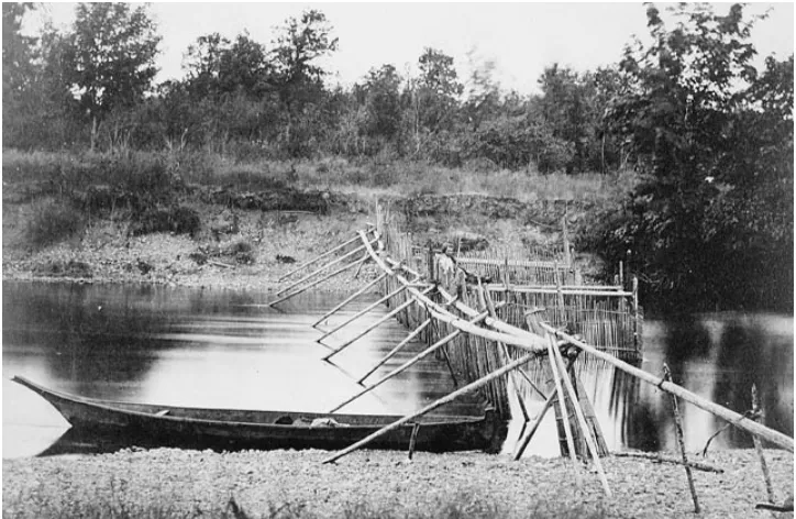
downstream. In Nevada, streams are small and snow fed, and thus, the stake and net method was employed by the Early Necada Paiute Indians. The fisherman would sit and wait at the center of the weir with a net. As the fish came to the weir, they would travel upstream towards the apex to find a way through. There, the fisherman could catch multiple fish with a net (Gilmore 1953). Salmon weir at
Quamichan Village on the Cowichan River, Vancouver Island, circa 1866 is shown in Figure 1.3.
Figure 1.3 Salmon weir at Quamichan Village on the Cowichan River, Vancouver Island Source: “Fishing Weir” 2007
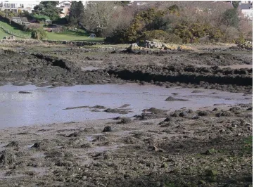
Figure 1.4 Stone Fish Weir on Menai Strait Source: “Fishing Weir” 2007”
While those seen in North Carolina tend to have upstream apexes, the apexes of many riverine fish weirs found in the literature are downstream (Lutins 1992). Weirs with the apex downstream would be better suited for catching fish migrating
downstream that were carried downstream by the current (such as eel as cited by Lutins 1992) or herded downstream into the gap at the apex. Fish weirs with the apex downstream would also direct flows outwards thus create a current that would carry the fish towards the banks. Weirs with the upstream apex would be better suited to catch fish migrating upstream. In these cases, fish could be trapped in the center with a net or basket, otherwise, they would be caught along the banks. It would be easier to spear them from the banks than to take out canoes to the center to catch the game.
folklore. “How Coyote Destroyed the Fish Dam at the Cascades: Distributing
Salmon in the Rivers” was recorded in October 1916. This particular story told how a coyote destroyed a fish trap at Celilo Falls, Oregon so that people upstream would also be able to fish (Trafzer 2005). Another story told by the Snoqualime Indians of Washington State described how the moon turned a fish trap into a waterfall to establish order among the people saying, “’Game of every kind shall be found by the people for their sustenance’” (Tollefson 1993).
There have been very few fish weirs researched and mapped in North Carolina (Lutins 1992). However, there are several documentations of such structures on historic sites as well as paddlers’ guides and archeological surveys. These are listed in Table 1.1.
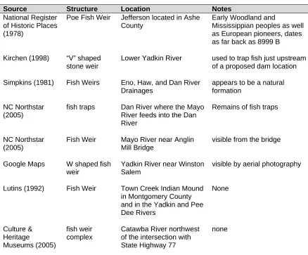
Table 1.1 Citations of Fish Weirs and Related Structures in North Carolina
Source Structure Location Notes
National Register of Historic Places (1978)
Poe Fish Weir Jefferson located in Ashe County
Early Woodland and
Mississippian peoples as well as European pioneers, dates as far back as 8999 B
Kirchen (1998) “V” shaped stone weir
Lower Yadkin River used to trap fish just upstream of a proposed dam location
Simpkins (1981) Fish Weirs Eno, Haw, and Dan River Drainages
appears to be a natural formation
NC Northstar (2005)
fish traps Dan River where the Mayo River feeds into the Dan River
Remains of fish traps
NC Northstar (2005)
Fish Weir Mayo River near Anglin Mill Bridge
visible from the bridge
Google Maps W shaped fish
weir
Yadkin River near Winston Salem
visible by aerial photography
Lutins (1992) Fish Weir Town Creek Indian Mound
in Montgomery County and in the Yadkin and Pee Dee Rivers None Culture & Heritage Museums (2005) fish weir complex
Catawba River northwest of the intersection with State Highway 77
While many stone fish weirs have been washed out or destroyed, many are still intact. It has been nearly 200 years since the early 1800’s Trail of Tears and the movement of Native Americans to reservations which leaves nearly two centuries of nature’s forces tearing at the structures since the last of the Native Americans would have been able to make repairs and adjustments to the structure. Not all of the remaining fish weirs are fully intact. It is possible to make out the general shape of a weir without having all the stones present. Lacking historical documentation, it is be difficult to determine the original height of the weirs. That aside, there must be a reason why they are not all completely washed out. One explanation is these fish weirs were constructed in fairly shallow waters, with the stones visible to barely visible during base flow. Base flow does not likely have the power to move these stones. The stress acting on the bed is related to the water depth and water surface slope. Because the stream is shallow, during high floods, the flow spills over onto the flood plain. This prevents very deep fast flows that might easily move large stones.
While the stone fish weir is functional either with the apex upstream or downstream, the rock cross vane would lose a major function by being inverted. The arms are able to protect the banks at low flow by forcing flow towards the center as the overflow surface of the arms angle the water inwards, away from the banks. At higher flows, the rock protects the bank as a barricade and by directing flow over the vane towards the center as with lower flows. The fish weir, from observation of photographs, does not appear to have arms that increase in elevation as they extend downstream. The fish weir does have a slight opening at the apex, but otherwise is partially above the water surface for the rest of the vane with water flowing through the cracks between stones. Instead of constricting flow and directing flow away from the banks causing a concentrated flow in the center, the vane
and have less of a hydraulic impact than the cross vane. However, there is striking similarity in shape and the use of vanes to turn water at the higher flows. While the Native American tribes that built fish weirs may not have been focused on bank protection in the development of their structures, they understood the concept of harnessing flow to serve a human purpose.
Dujiangyan Irrigation Scheme of ancient China
Another culture with a deep history with flow manipulation is the Chinese culture. The oldest know irrigation system is the Dujiangyan Irrigation Scheme of ancient China in the Sichuan Province. It was constructed in 256 BC by Li Bing, the governor of Shu. The three major parts of the Dujiangyan Irrigation Scheme
headworks are: Dujiang Yuzui (fish mouth), Feishayan, and Baopingkou, consist of a 1) diversion dam, 2) a spillway and 3) an intake which work to, respectively, 1) divide the river in two, 2) control silt and sediment during floods and 3) provide a steady flow (Li 2006). According to Li and Xu (2006), “It is a model of harmonious
coexistence between mankind and nature, and is also included as a World Heritage Site by the United Nations Educational, Scientific and Cultural Organization
(UNESCO) as the first water project in the world”.
Horseshoe Weirs
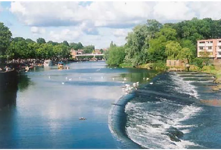
Figure 1.5 Chester Weir on the Dee River Source: “River Dee, Wales” 2007
Chester Weir was rebuilt in 1281 after damage from a flood. Horseshoe Falls also on the Dee River of Wales is a horseshoe weir constructed in 1808 by civil engineer Thomas Telford (Cragg 1997).
Evolution of the Rock Cross Vane
In the United States, river work and maintenance began in the late 1800’s to early 1900’s. In 1887, Congress established the Mississippi River Commission to address the needs for improvement as a result of highly damaging floods in 1849 and 1850 (USACE 2007). In the Western United States, around 1925 stream maintenance effort continued with the development with levee systems and dams on the Colorado River in Yuma, Arizona (LCRMSCP 2004). The term “stream and river restoration” is not in reference to manipulation of waters for public use, but rather to water quality and habitat improvements. White (1996) attributes the first American stream
moved to the west where wood and boulder structures were implemented to reverse the effects of logging, soil cultivation, and grazing (White 1996). It is hard to
determine exactly when this work began in the United States, especially as it relates to in-stream structures; however, Duff and Banks (1988) conducted a
comprehensive literature review as a means of documenting the history of stream restoration as it relates to improving fish habitat. They classify in-channel structures as habitat management, which were second to bank stabilization practices.
In-channel structures were mentioned in 68% of articles since 1970 and 46% of articles since 1980 (Duff and Banks 1988).
Design guidelines for rock cross vanes were first documented by Dave Rosgen in 1996 and arose out of a need for softer forms of bank protection (Rosgen 2001). Soft typically refers to banks that have not been hardened by the application of rip-rap or similar practices. Efforts from the Army Corps of Engineers and researchers and practitioners such as Richard Hey and Dave Rosgen have explored a variety of measures which have included hardening of the banks with boulder structures and flow redirection as well as combinations of the two.
1980’s Rock Vortex Weirs and Rootwads
Figure 1.6 Plan View of Rock Vortex Weir Source: Stormwater Manager’s Resource Center 2007
Figure 1.7 Plan View of Rootwad Revetment Source: Stormwater Manager’s Resource Center 2007
Rosgen (1996) states that after fifteen years of monitoring, rootwads actually lead to worse bank erosion during high flows due to eddies. While eddies provided nice areas of scour for fish, the associated scour became problematic when it lead to bank instabilities. Root wads are still commonly used and are often installed in combination with other structures as a way to increase woody debris in the stream and protect banks.
1988 The Bendway Weir
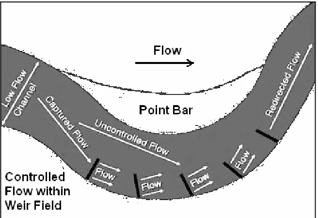
The United States Army Corps of Engineers (USACE) warns against the angle approaching parallel to flow lest it is behaves more as a flow divider. This is a problem commonly seen at the arms of rock cross vanes placed in a bend, where the flow attempts to bypass the arm and scours out the adjacent bank. Figure 1.8 is a diagram that demonstrates the concept of the bendway weir.
Figure 1.8 Bendway Weir Theory Source: Adapted from USACE 2006
Mr. Thomas J. Pokrefke Jr. initially conceived the bendway weir for use in a model of the Mississippi River. According to a publication produced by the USACE Costal Hydraulics Laboratory, the model addressed the following problems via subsequent solutions:
2. Constricted navigation channel via a widened channel through the bend and downstream of the bend
3. High velocities via controlled flow and increased weir effectiveness at high flow and high energy conditions
4. Damaging high-flow current patterns via increased uniformity of surface velocities
5. Insufficient navigation channel widths in the crossing downstream of the bend via the widening mentioned earlier and a flow path moved towards the inside bend
6. The loss of Least Tern nesting areas via improvements to aquatic habitat and bank stabilization (USACE 2006).
1987- 1989 Iowa Vanes and Submerged Concrete Vanes
Figure 1.9 Installation of Concrete Iowa Vanes at Low Flow Source: “How to Control Streambank Erosion” 2006
Several years after the initial theoretical designs were made, Paice and Hey (1989) introduced the use of submerged concrete vanes which would not only control the secondary circulations to protect the banks but provide much needed fish habitat (Rosgen 2001). The supplemental function of fish habitat was one of the driving factors that would later appear in the goals of the rock cross vane.
1990’s Rock Cross Vane
The rock cross vane is best applied to stream restorations where flood plane restrictions limit increasing stream sinuosity to decrease bed slope. The drop
Figure 1.10 Plan View of Rock Vane and J-Hook Source: Stormwater Manager’s Resource Center 2007
The arms protect banks by turning water towards the center of the stream which results in scour pool development. Ironically, the rock cross vane was observed to carry a high risk of bank erosion both at the arms of the structure and downstream of the structure in Chapter 4 of this study. Bank erosion was primarily attributed to side cutting as a result of alignment, placement, and undersized rock cross vanes.
The rock cross vane is both a weir and a vane. It is somewhat similar to a duckbill weir and a labyrinth weir, which are both long-crested weirs. Long crested weirs are those that have a longer overfall length than the actual width of the channel. Figure 1.10 is of three types of long crested weirs.
The labyrinth weir is the only weir in Figure 1.11 that is not contracted. A difference between the three long crested weirs above and the rock cross vane is that the weirs have a constant crest elevation. Rock cross vane arms increase in elevation in the downstream direction. The flow area over the rock cross vane is shaped most like a Cipolletti weir. This is deceptive because the water is not only flowing in one
direction and the overflow surface is much longer than in the front view of the vane. These inclined arms are what give the rock cross vane the “vane” part of its name.
Present-day Challenges
The focus on restoring streams and rivers to a “natural” state has resulting in the development of small structures that can blend in with the environment. Structures are built with materials that could be found in proximity to the stream such as logs and boulders (as opposed to steel and concrete). Boulder vanes (cross vanes, j-hooks, single arm vanes, rock vortex weirs, etc) provide a measure of stability dependent on the design of the structure, the placement and construction, and largely on the experience of the designers and construction contractors as well as chance – not the most preferential tool to work with. Streams and rivers migrate slowly over time. Sometimes they migrate rapidly in cases of severe environmental events and changes.
The evolution of structures used for stream stability has not necessarily led to more durable or effective practices. Many structures are altered on a trial and error basis and lack a methodical approach is not used due to a poor of understanding of stream functions. Rosgen (2001) states,” Structures in river engineering are designed to help stabilize channel boundaries. However, monitoring their
effectiveness have indicated that many structures, contrary to the intended design, caused river instability. Structures are often selected and installed without an
Rock cross vanes are designed according to a standard plan and are sized
according to bankfull width. The standard range of slopes and arm angles are used to provide flexibility in tying arms to bankfull when possible. Monitoring has shown that these structures can cause a variety of problems around the vane which may influence stream and river instability (Rosgen 2001). Highly eroding banks around structures disturb the sediment balance downstream and change the geometry of the channel at the structure.
Rock cross vanes are designed to mimic natural rock outcroppings. The formation of a waterfall occurs in a similar fashion to the upstream migration head cut past a failed rock cross vane. Figure 1.12 is a diagram of the formation of a waterfall.
Figure 1.12 Formation of a Waterfall Source: Mann 2006
layer of hard rock results in slower upstream migration of the headcut. Because the sill is usually only one boulder thick along the bed, once the sill is bypassed, headcut migration occurs more rapidly. Rock structures “harden” banks and actually
accelerate bank erosion as they begin to fail (Rosgen 2001).
In nature, drop structures change over time. In pristine systems where there is little human presence, watersheds are mostly stable, and change occurs slowly. Stream restoration is conducted in regions of minor to severe human intrusion where the watershed can be rapidly changing. Researchers should expect and design for, at the least, the changes that occur in nature. There should be efforts to develop in-stream structures that tolerate change over time. Streams are dynamic systems and should include structures that are dynamic as well. It is unreasonable to expect hard fixed structures to remain intact and functional in an unstable environment.
The following chapters explored the nature of the rock cross vane – how it
redistributes the velocity profile, its most common paths of failures, and its design inadequacies – in an effort to improve upon and advance the technology. The
Literature Cited
“Bendway Weirs.” Coastal and Hydraulics Laboratory - Engineer Research and Development Center. USACE. Available at:
http://chl.erdc.usace.army.mil/chl.aspx?p=s&a=ARTICLES;109. Accessed 28 November 2006.
Cragg, Roger. 1997. Civil engineering heritage: Wales and west central England.
London: Thomas Telford Ltd for Institution of Civil Engineers.
Gilmore, H. W. 1953 . “Hunting Habits of the Early Nevada Pauites.” American Anthropologist, New Series, 55(1): 148-153.
“Fishing Weir.” Available: http://en.wikipedia.org/wiki/Fish-weir. Accessed 19 March 2007.
Hatcher, R. D., Howell, D. E., and Talwani, P. 1977. “Eastern Piedmont fault system: Speculations on its extent.” Geology. 5: 636-640
“How to Control Streambank Erosion.” Iowa Department of Natural Resources. 2006. Available at:
http://www.iowadnr.com/water/stormwater/forms/streambank_man.pdf. Accessed 19 March 2007.
Kirchen, R. W. 1998. “Archeological Survey and Testing of the Yadkin Intake Dam Project Area, Prepared for the City/County Utilities Commission, Forsyth County, North Carolina.” Wake Forest Archeology Laboratories.
Li, K. and Xu, Z. 2005. “Overview of Dujiangyan Irrigation Scheme of ancient China with current theory.” Irrigation and Drainage. 19th ICID International
Congress, Beijing, 55(3):291-298.
Lutins, A. H. 1992. “Prehistoric Fish Weirs in Eastern North America.” Unpublished Masters thesis, State University of New York, Binghamton.
Lutins, A. H., DeCondo, A. P. 1999. “The Fair Lawn/Paterson Fish Weir” Bulletin of the Archaeological Society of New Jersey, 54.
National Register of Historic Places (NRHP) 2005. Available:
www.nationalregisterofhistoricplaces.com. Accessed 20 August 2005. “Natural & Cultural Features of the McColl Property” Culture & Heritage Museums.
Odgaard, A. J. “Iowa Vanes – An Inexpensive Sediment Management Strategy.” The University of Iowa. Available at:
http://www.iihr.uiowa.edu/projects/IowaVanes/index.html. Accessed 28 November 2006.
Odgaard, A. J., and Kennedy, J.F. 1983. “River-bend bank protection by submerged vanes.” J. Hydr. Engrg., ASCE, 109 (8): 1161-1173.
Odgaard, A. J., and Spoljaric, A. 1986. “Sediment control by submerged vanes.” J. Hydr. Engrg., ASCE, 112 (12): 1164-1181.
“River Dee, Wales.” Available at: http://en.wikipedia.org/wiki/River_Dee%2C_Wales. Accessed 19 March 2007.
“Rockingham County River Country” NC Northstar. Available at:
http://www.ncnorthstar.com/rc_rwebsections.shtml. Accessed 18 July 2005. Rosgen, D. L. 2001. “The Cross-Vane, W-Weir and J-Hook Vane Structures...Their
Description, Design and Application for Stream Stabilization and River Restoration.” Wildland Hydrology, Inc. 22 pp.
Simpkins, D. L. and Petherick , G. L. 1986. “Second Phase Investigations of Late Aboriginal Settlement Systems in the Eno, Haw, and Dan River Drainages, North Carolina” Research Report No. 6. Research Laboratories of
Anthropology, The University of North Carolina at Chapel Hill. Stormwater Manager’s Resource Center. Available at:
http://www.stormwatercenter.net. Accessed 19 March 2007. “The Mississippi River and Tributaries Project.” USACE. Available at:
http://www.mvn.usace.army.mil/pao/bro/misstrib.htm. Accessed 19 March 2007.
Tollefson, K. D. and Abbott, M. L. 1993. “From fish weir to waterfall. (Snoqualmie Falls' significance to Snoqualmie Tribe)” The American Indian Quarterly. Trafzer, C. E., ed. 1998. “Grandmother, Grandfather, and Old Wolf: tamánwit ku
súkat and traditional Native American narratives from the Columbia Plateau.” Michigan State University Press.
Mann, J. C. “Formation of a Waterfall.” Wikipedia. Available at:
http://en.wikipedia.org/wiki/Waterfall. Accessed 28 November 2006.
University of Wyoming, May 1993. Available at:
Chapter 2:
Effects of Rock Cross Vane Geometry on Velocity
Distribution
Abstract
This flume study assessed the velocity ratio (average center velocity to average outer velocity) influenced by a range of rock cross vane geometric variables implemented in practice. A stream segment was modeled with a rectangular channel. A fractional factorial design of three geometric variables the cross vane was tested in a flume study at North Carolina State University. Results showed linear and quadratic effects of drop ratio (drop depth to bankfull depth), and interaction effects of arm angle and drop ratio, arm slope and drop ratio, and arm slope and arm angle on the velocity ratio. The area of flow at the overfall of the structure was calculated and compared to the area of the drop without the structure. This area ratio (flow at structure to flow of simple drop) was used to predict whether constriction or overtopping of bankfull conditions was occurring. Calculations of flow area at the overfall predicted flow constriction over the structure at a high arm slope within the prescribed ranges of arm slope (0.03 – 0.07) and arm angle (20 – 30 degrees). Results of the flume study and area calculations imply that sufficient drop is essential to creating the higher velocity ratios necessary for scour pool
Introduction
Functions of the Rock Cross Vane
The main function of vanes in rivers and streams is to change the direction of the flow of water. The rock cross vane combines 1) flow redirection, 2) grade control, and 3) scour pool development. The vertical drop and vane-like arms direct the water towards the center of the channel causing flow to be slowed near the banks and a pool to be scoured just downstream of the rock cross vane.
Geometric Variables of the Rock Cross Vane
There are four main geometric components of the rock cross vane: arm angle, arm slope, drop, and width ratio of arms to center of the vane. The first three are
accompanied by accepted ranges. The fourth is fixed. Referring to Appendix A and Figures A-1 and A-2, the following definitions and recommendations of arm angle and arm slope are given:
1. Arm angle is measured where the arm projects from the downstream bank. The range prescribed by most designers is a 20 to 30 degree angle.
2. Arm slope is measured as the rise from the horizontal over run of the top surface of the arm. The upstream end of the arms of the vane is at a lower elevation than the downstream end. The arm slope range prescribed by most designers is 3 to 7%. Ideally, the arms of the vane tie in at bankfull; however, a low slope vane will tie in at a lower level than a high slope vane for a fixed arm angle.
drop is a term used to describe the drop and the pool depth. Effective drop is not used in this study.
Rock cross vanes are designed such that both arm and sill comprise one-third of the bankfull width of the channel. This study addresses the first three components of cross vane geometry which are varied in practice.
The Current Problem with Rock Cross Vane Design Recommendations
The effects of the given ranges of the geometric variables of the rock cross vane on velocity distributions of flow have not been modeled. Dave Rosgen, the first to publish design recommendations and diagrams for rock cross vanes and other structures, has updated some of his rock cross vane designs (Rosgen 2004). His diagrams of the cross vane design in his 2001 publication are commonly used in North Carolina streams and are the focus of this study (Figure A-1 and Figure A-2 of Appendix A). Recommendations for rock cross vanes are constantly changing, and the design of the rock cross vane will continue to evolve. Currently, design
judgments in practice are made based on a combination of required durability and function. Changes to the design are made when observations show that the rock cross vane is not performing as expected. Rather than develop the structure based on trial and error, it would be better to determine the optimum design for the rock cross vane through careful testing. This study focused on one aspect of rock cross vane performance: the effects of the design variables on the velocity distributions upstream and downstream of the structure.
Hypothesis and Study Goals
It was observed in this study and by other practitioners that higher arm angles tended to be coupled with more sediment deposition at the end of the arms.
by increased eddies at higher arm angles. Rock cross vanes with higher arm slopes have been observed to form deeper pools, leading to the inference that they too cause greater flow concentration in the center of the stream. It has been observed that higher drops form deeper pools, and it was hypothesized that the effects of drop height on the velocity ratio could be due to a stronger impingement jet and a
changed flow distribution. It was hypothesized that the design variables of the rock cross vane have significant effects on the upstream and downstream velocity distributions. It was also hypothesized that there are potential values of these variables that would have adverse effects on rock cross vane performance due to reduction of flow area over the structure. These values were estimated, but negative effects such as bank erosion were better observed by visual inspection of actual structures in streams.
There were two main goals of this study:
1. To explore and quantify the effects of the design variables arm angle, arm slope and drop ratio on the flow distributions up and downstream of the rock cross vane with a physical model.
2. To apply the knowledge gained about the effects of geometry with recommended improvements to the design of the rock cross vane and recommend future research.
Effects of Geometric Change on Velocity Distribution
Bank protection occurs downstream because the flow near the banks is slowed down. Scour pool development occurs because of the jet impingement and
Figure 2.1 Plan View of the Velocity Distributions at Rock Cross Vane
One way to quantify the resulting shape of the velocity distribution is to compare the center velocity to the outer velocity. The term velocity ratio is used to quantify the comparison of the two velocity regions. Velocity ratio is the ratio of the average center velocity to the average outer velocity. In Figure 2.1, this translates to the average of the velocity at points 2, 3, and 4 to the average of points 1 and 5. The averages account for a lack of symmetry in the velocity distribution.
By knowing the relationship of the rock cross vane’s arm angle, arm slope, and drop ratio, a designer may use the predicted mean velocity to calculate the velocities near the banks and in the center of the stream. This would allow the designer to predict potential bank erosion and scour pool development. This study sought to find the optimum arm slope, arm angle, and drop ratio combinations to maximize the velocity ratio.
Potential Adverse Effects of the Rock Cross Vane on Flow
slopes reduces the flow area over the structure for a fixed depth. For this study, area ratio was defined as flow area at the overfall of the rock cross vane to the flow area at the overfall of a simple drop without the structure. When this ratio is less than one, there are two possible conditions: (A) the flow is constricted, or (B) the water surface elevation has increased and flow has overtopped the structure, depending on the flow and channel conditions. A simple impediment of a step in the channel can be used to simplify what is occurring with the rock cross vane. Figure 2.2 is a diagram of a step in a channel.
Figure 2.2 Diagram of a Step in a Channel
constriction over the arms of the rock cross vane is increased velocities against the adjacent banks and the bed of the boulders causing scour and erosion. There were cases in the flume study where constriction was likely occurring. The risk of the structure overtopping, which is expected for larger storm events that the bankfull (1.5 year return interval), is that upon re-entry scour occurs on the banks at the ends of the arms of the structure. If this is frequently occurring, it can eventually lead to side cutting and a decrease in structure durability.
Hydraulic Jump at the Rock Cross Vane
Hydraulic jumps have been observed downstream of rock cross vanes. The jump helps dissipate energy and create the scour pool.
Chow (1959) developed methods for developing a drop number DN and depths
surrounding the hydraulic jumps based on the following equations:
3 2
gh q
DN = (1)
Where,
q = Unit discharge, cfs/ft h = Effective height of drop, ft.
From the drop number, drop length, pool depth under nappe, depth of upstream of the hydraulic jump and downstream depth can be determined.
27 . 0 30 . 4 N D D h L
= (2)
22 . 0 00 . 1 N D D h y
= (3)
425 . 0 1 0.54
N
D h
y
27 . 0 2
66 .
1 DN
h y =
(5)
Where,
LD = Jump length, ft
yD = Pool depth under nappe, ft
y1 = Depth upstream of the hydraulic jump, ft
y2 = Subcritical subsequent depth, ft.
Figure 2.3 is a schematic of a hydraulic jump. In the physical model, there was no pool under the nappe, so yD is not depicted.
Figure 2.3 Hydraulic Jump
The length of the drop can be calculated from Equation 2 or from the Froude number and Figure 2.2
1 1
v Fr
gy
= (6)
Where,
Figure 2.2 is used to estimate the length of the hydraulic jump.
Figure 2.4 Length of Jump for a Rectangular Channel Source: FHWA 2007
The drop over the rock cross vane is not rectangular as it is assumed to be in Chow’s equations. Flow dropping from the length of the arms is directed inward towards the center of the channel. It is possible that the jump may be experienced further downstream than that which is calculated for a rectangular drop as flow may drop off the full length of the arm. This complicates the calculations of the expected depths and length of the hydraulic jump.
Related Studies
the relationship between the vane geometry and the resulting downstream pool length, depth and location. This study is observational (Lawrence 2006). A graduate student from New York, Margaret M. Soulman, recently studied 12 cross vanes constructed on the Batavia Kill in the Catskills. Soulman studied the cross vane geometries and the greater stream context to better understand the variability in the pools depths below the cross vanes. She found connections between the arm slopes and the pools’ width/depth ratios and an even stronger connection between the arm width – center width ratios and the width/depth ratios (Soulman Email correspondence 2 June 2005).
A structure similar in function to the rock cross vane, the bendway weir, is used on the outside of bends to reduce outer bank velocity and push flow back towards the centerline. This results in deepened channels and stabilized bank erosion. Thornton et al. conducted a flume study to test how different designs of the weir affected the outer bank velocity to center velocity ratio. They modeled two bends on the Middle Rio Grand reach with Froude similitude at a 1:12 scale. A Sontek Acoustic Doppler velocimeter was used to measure the point velocities (Thornton et. al. 2005). Their measure of velocity ratio was used in this study as a good way of quantifying the shape of the velocity distribution. They used three ratios: 1) the maximum outer bank velocity to the maximum center baseline velocity, 2) the maximum inner bank
velocity to the maximum center baseline velocity, and 3) the maximum center velocity to the maximum center baseline velocity.
Materials and Methods
Site Layout and Flow Source
The test site was located at the NCSU Lake Wheeler Road Field Laboratory in Raleigh, NC. The flume received flow from a storage pond located uphill of the flume. The flume testing site is shown in Figure 2.5.
The inflow pipe for the flume had a one foot diameter. Table 2.2.1 gives the slope and length of the inflow pipe and the initial water elevation in the pond for tests.
Table 2.1 Pipe Elevation, Length, and Slope
96.13 Pipe elevation in pond, ft 83.65 Upper pipe length, ft 94.95 Pipe elevation at juncture, ft 83.74 Lower pipe length, ft 92.99 Pipe outlet elevation , top, ft 0.0141 Upper pipe slope, ft/ft 3.14 Total Drop, ft 0.0234 Lower pipe slope. ft/ft
167.39 Length of pipe, ft 99.78 Initial water elevation in pond, ft
The storage pond was surveyed and Malcom’s (1989) methods were used to
calculate the stage-storage of the pond and to model the expected discharge coming out of the pipe using Malcom’s Chainsaw Method (1989) in Table 2.2. The
coefficient of discharge used for the pipe was 0.6 and the weir coefficient, Cw, was 3.33.
Table 2.2 Time Discharge Calculation
T, min Qin, cfs S, cu.ft. Z, ft. Qout, cfs
0 0 6776 3.65 6.70
1 0 6374 3.51 6.55
2 0 5981 3.36 6.39
3 0 5598 3.22 6.23
4 0 5225 3.08 6.06
5 0 4861 2.93 5.89
6 0 4508 2.79 5.72
7 0 4165 2.65 5.54
8 0 3833 2.51 5.35
9 0 3511 2.37 5.16
10 0 3202 2.23 4.96
11 0 2904 2.09 4.76
12 0 2618 1.95 4.55
13 0 2345 1.82 4.33
14 0 2085 1.68 4.10
15 0 1839 1.55 3.86
1.5 2 2.5 3 3.5 4
0.0 5.0 10.0 15.0
time (min)
st
ag
e (
ft
)
observed calculated
Figure 2.6 Observed Stage vs. Time of Storage Pond Drawdown
The slightly flattened portion of the observed stage-time relationship at time zero to ten seconds was caused by the opening of the electro-mechanical actuated valve (refer to Figure 2.4). Drawdown was slower than predicted which could have been caused by algal blockages at the outlet or friction losses through the valve.
Flume Design
The flume design and testing methods provided a physical model that was a
simplified model of a stream of equal size with a length ratio of 1:1. All the variables (arm angle, arm slope, and drop ratio) were dimensionless. The response variable, velocity ratio, was also dimensionless. This eliminated scale effects and made the model applicable to streams of a similar width/depth ratio and flow regime. A rectangular flume was chosen for construction purposes.
lowered by jacks to change the height and therefore drop ratio. The upper segment was 20 ft long, and the lower segment was 24 ft long. Bed slopes were constant throughout the study, while the drop between them varied.
The chosen bankfull width/depth ratio was 14:1, which fell into the C channel
Figure 2.7 Plan View of Test Flume
walls and bed. The installation of marine carpet resulted in a relatively low Manning’s n value that fell between the planed wood Manning’s n of .012 and the short grass value in a dredged channel of 0.022 (Chow 1959). In order to check the chosen Manning’s n, the normal depth ranges in the upper and lower flume were calculated by using the Manning’s n range (.012 - .022). Normal depth was calculated for the given slopes and channel dimensions under the assumption that the flume segments were hydraulically long enough to achieve normal depth conditions. The upper
segment average depth was taken at Cross Section A during base conditions. The lower segment average depth was taken at Cross Sections B and C during base conditions. Base conditions were the running of the model with the drop without arms. This is shown in Table 2.3.
Table 2.3 Predicted Normal Depth and Observed Depth
Predicted Depth
Flume segment n=.012 n=.022 Observed average Depth upper 0.20 ft 0.29 ft 0.43 ft
lower 0.22 ft 0.32 ft 0.30 ft
In the upper flume, flow was deeper than the predicted values of depth for Manning’s n. This can be attributed to sagging in the upper flume. Although not planned, the sagging was appropriate for the physical model because oftentimes, rock cross vanes are installed at the ends of pools. In the lower flume, the average observed depth fell within the predicted depth range given the Manning’s n between 0.012 and 0.022. The best guess for Manning’s n in the flume is 0.02, interpolated from the lower flume average depth and the predicted depths for the range of Manning’s n.
positioned on the bed of the downstream segment. Arm slope was fine-tuned by adding shims and blocks. Figure 2.8 is the profile view of the location of the arms between the upper and lower flumes.
Figure 2.8 Profile View of Rock Cross Vane Model
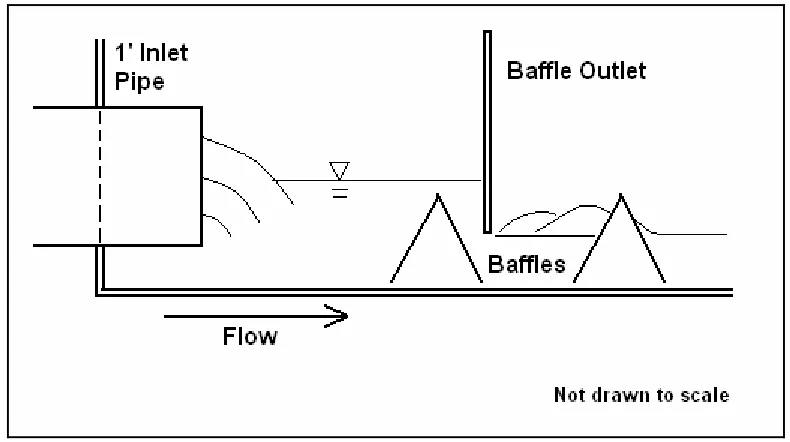
Another component of the flume was added at the head of the flume:
1) A baffle outlet to help reduce the effects of head changes in the basin due to flow rate changes.
2) Triangular flow baffles or dissipaters, which helped create a uniform velocity distribution at the head of the flume.
Figure 2.9 Profile View of Flume Stilling Basin and Baffle Outlet – Baffle Combination
Velocity Test Points Locations and Methods
Velocity was measured with a USGS Pygmy Meter Model 6205 and an AquaCount Calculator shown in Figure 2.11. Figure 2.6, indicates where test points were taken.
Figure 2.11 Test Run with the Pygmy Meter and AquaCount Calculator
Velocity was measured over 20 second intervals at each of the five points across each of the three cross sections. The cross sections were located as follows: (A) one bankfull width (6.5 ft) upstream of the beginning of the vane, (B) one bankfull width downstream of the beginning of the vane, and (C) two bankfull widths
downstream of the beginning of the vane. The points were located so that each was in the center of five equally spaced segments across the width of the flume: 0.66 ft, 1.98 ft, 3.30 ft, 4.62 ft, and 5.64 ft.
this measurement the elevation survey taken at each point across the cross sections to account for minor elevation changes across each cross section. Flow rate was calculated from the average velocity and depth. There were hydraulic jumps coming off the sill and both arms which collided in the middle of the structure or expected pool region. The shape of and distance to the hydraulic jump varied with the drops and arms widths and slopes and were not measured.
Figure 2.12 shows the cross vane with water flowing from the bottom of the picture to the top.
Figure 2.12 Flume test of drop ratio = 1, angle = 20˚, slope = 3%
Testing for Effects of Time Variations during Velocity Measurements
The ideal flume test would have lasted under six minutes with initial and final discharges of 6.7 cfs and 5.7 cfs respectively, as estimated from Table 2.2.
distribution of a cross section was not done at the same time point during the pond draw down, flow distributions would not be represented accurately because the flow coming from the inlet pipe would be less, and there would be a lower energy head. The velocity distribution at each cross section was measured three times over a pond drawdown. This was replicated three times for a total of nine test runs. These tests showed that velocity ratios at the cross sections were unaffected by the stage-time effects during a run. See Table 2.4 below.
Table 2.4 Velocity Ratio for Three Test Runs at each Cross Section
For each test run at the cross sections, velocity ratio was measured three times. Velocity Ratio was measured as the average center velocity – points 2, 3, and 4 - divided by the average outer velocity – points 1 and 5.
Cross Section – Test Run
Velocity Ratio Measurement 1
Velocity Ratio Measurement 2
Velocity Ratio Measurement 3
A – Test Run 1 1.21 1.25 1.17
A – Test Run 2 1.29 1.29 1.34
A – Test Run 3 1.26 1.26 1.34
B – Test Run 4 1.20 1.07 1.14
B – Test Run 5 0.98 1.02 0.97
B – Test Run 6 1.02 0.99 1.00
C – Test Run 7 1.32 1.30 1.44
C – Test Run 8 1.53 1.42 1.48
C – Test Run 9 1.40 1.33 1.39
B. Minor leakages occurred during the length of the lower flume which accounts for the minor difference in flow rate between cross section B and C.
Experimental Design
The experimental design was a factorial analysis where each variable was tested at three values. Table 2.5 lists the values for each of the three levels of each variable in the study.
Table 2.5 Factor Levels and Values
Factor Level
Arm Angle (deg)
Arm Slope (ft/ft)
Drop Ratio (ft/ft)
1 15 0.01 0.25
2 25 0.05 0.75
3 35 0.09 1.25
This resulted in a total of 27 combinations of variables tested in the flume with three test runs each which acted as replications for statistical purposes. Also tested were the velocity distributions across the three cross sections at each drop without the arms attached. This was referred to as base condition. This was included so that the effects of the inclusion of arms on the depth of flow could be observed. All test points are included in Table A-1 of Appendix A.
Calculation of Flow Area of over the Rock Cross Vane
The area over the arms is calculated as twice the average depth over one arm multiplied by the water surface length over one arm. The average depth of water on the arms is the average of the depth over the end of the arm and the depth of flow where the arm connects at the sill. The depth at the end of the arm is the difference between the depth of flow and the elevation of the arm at that point which can be calculated by the given arm slope, angle and width, shown in the first part of Equation 7. The length of the overflow surface is the horizontal projection of the length along the diagonal of the arm, which is the water surface length over the arm. This is calculated from the given arm slope and arm angle as shown in the second part of Equation 7, which assumes arms are fully inundated.
2 2 ) tan( ) cos( ) tan( ) sin( 2 ⎟⎟ ⎠ ⎞ ⎜⎜ ⎝ ⎛ + ⎥ ⎦ ⎤ ⎢ ⎣ ⎡ − = α α s W W s W h A arm arm arm arm
arms (7)
Where,
harm = depth of flow over the arms, ft
α = angle of the arm from the bank, degrees
s = slope of the arm from the horizontal, degrees
Warm = width of arm laterally across the stream, ft
Equation 8 gives the adjusted lateral arm width for conditions when the arm is not fully inundated. ) sin( ) tan( s h W sill new α
= (8)
Where,
hsill = depth of flow over the sill
Flow area over the sill is calculated as the depth of flow multiplied by the width of the sill.
sill sill sill h W
Where,
Wsill = width of sill, ft
Total area at the overflow surface of the rock cross vane is:
sill arms total A A
A = + (10)
The depth of flow at the overfall is actually shallower than the upstream depth. As water flows over the rock cross vane, two different depths can occur. When there is a free overfall, water flows over a brink at a depth known as brink depth. When the drop is low enough that the tail water depth prevents a free-overfall, the structure’s arms behave as broad crested weirs and flow is at critical depth.
Critical depth, yc is calculated from Henderson (1966) as:
3 2 g q
yc = (11)
Brink depth is estimated as:
c brink y
y =0.7 (12)
Plugging this estimated for depth over the arms and sill gives an estimate of the flow area over the rock cross vane. Expected flow area without the structure is simply the multiplication of the brink depth and channel width. These equations were used to predict potential constriction through the rock cross vane at a drop ratio of 0.75.
Results and Discussion
Velocity Ratios Observed
Table 2.6 Velocity Ratio for Cross Section by Test Run
VRA is the velocity ratio at cross section A. VRB is the velocity ratio at cross section B. VRC is the velocity distribution at cross section C. D = drop ratio. A = arm angle. S = arm slope. 1,2,3, indicate factor levels (see Table 2.5). VRA = velocity ratio at cross section A. VRB = velocity ratio at cross section B. VRC = velocity ratio at cross section C.
Test Run VRA VRB VRC Test Run VRA VRB VRC
Statistical Modeling
PROC GLM LSMEANS was run to determine whether the cross sections were statistically different shown in Table 7. Pdiff with Tukey test showed that the cross sections had significantly different means (p<0.0001).
Table 7 LSMEANS for Class Effects of Cross Section
Cross Section LSMEANS 1 – Cross Section B 2.66575 2 – Cross Section C 1.77396 0 – Cross Section A 1.18826
PROC RSREG was run to model the linear, quadratic and interactive effects of the variables on the velocity ratio. Equation 13 is the response surface regression model of velocity ratio.
Slope Slope Angle Slope Drop Slope Angle Angle Drop Angle Drop Drop Slope Angle Drop Ratio Velocity 9 8 7 6 5 4 3 2 1 0 × + × + × + × + × + × + + + + = β β β β β β β β β β (13) Where,
Velocity Ratio = as defined in the introduction, ft/s / ft/s drop = drop ratio as defined in the introduction, ft/ft
angle = arm angle as defined in the introduction, degrees slope = arm slope as defined in the introduction, ft/ft
Figures 14 and 15 present the predicted velocity ratios by paired combinations of the three factors, drop, angle and slope. Drop effects were maximized just over 100% drop and begin to diminish.
15 20
25 30
35
Angl e 25
50 75
100 125
Dr op 1. 24
1. 52 1. 80 2. 08 2. 36 pr edi ct ed
Figure 2.14 Predicted Velocity Ratio versus Arm Angle and Drop Ratio for Cross Section C
25 50
75 100
125
Dr op 1
3 5
7 9
Sl ope 1. 24
1. 52 1. 80 2. 08 2. 36 pr edi ct ed
Figure 2.15 Predicted Velocity Ratio versus Drop Ratio and Arm Slope for Cross Section C Fit of Model
The model was run for all data by cross section. Based on the residuals plots, cross section C was the only model that was deemed to have a strong fit. The models for cross sections A and B did show significant effects of several variables, but the model cannot be used to accurately predict velocity ratio for these cross sections. While the model for cross section A seemed strong (R2 = 0.8749), the plot of
Figure 2.16 Residuals at Cross Section A
Table 2.8 presents the Analysis of Variance for the Response Surface Equation Model at Cross Section A.
Table 2.8 Analysis of Variance for Response Surface Regression Model at Cross Section A
Regression DF
Type I Sum
of Squares R-Square F Value Pr > F Linear 3 0.676991 0.6473 122.42 <.0001 Quadratic 3 0.203805 0.1949 36.85 <.0001 Crossproduct 3 0.034247 0.0327 6.19 0.0008 Total Model 9 0.915043 0.8749 55.16 <.0001
Vr at i o = 1. 8068 +0. 0101 Dr op - 0. 0241 Angl e +0. 0623 Sl ope - 0. 0001 dr op2 - 0. 0001 angl e2 +0. 0084 sl ope2 - 0. 0004 sd - 0. 0037 sa +0. 001 da
N 81 Rsq 0. 6537 Adj Rsq 0. 6098
RMSE
0. 4904
- 1. 00 - 0. 75 - 0. 50 - 0. 25 0. 00 0. 25 0. 50 0. 75 1. 00 1. 25
Pr edi ct ed Val ue
1. 50 1. 75 2. 00 2. 25 2. 50 2. 75 3. 00 3. 25 3. 50 3. 75 4. 00
Figure 2.17 Residuals at Cross Section B
Table 2.9 presents the Analysis of Variance for the Response Surface Equation Model at Cross Section B.
Table 2.9 Analysis of Variance for Response Surface Regression Model at Cross Section B
Regression DF
Type I Sum
of Squares R-Square F Value Pr > F Linear 3 19.86432 0.4029 27.54 <.0001 Quadratic 3 2.694427 0.0547 3.74 0.0149 Crossproduct 3 9.66647 0.1961 13.4 <.0001 Total Model 9 32.22521 0.6537 14.89 <.0001
Vr at i o = 0. 919 +0. 0223 Dr op - 0. 0189 Angl e - 0. 0031 Sl ope - 0. 0001 dr op2 +0. 0002 angl e2 +0. 0012 sl ope2 - 0. 0004 sd +0. 0011 sa +0. 0003 da
N 81 Rsq 0. 9139 Adj Rsq 0. 9030
RMSE
0. 1127
- 0. 3 - 0. 2 - 0. 1 0. 0 0. 1 0. 2 0. 3 0. 4
Pr edi ct ed Val ue
1. 2 1. 3 1. 4 1. 5 1. 6 1. 7 1. 8 1. 9 2. 0 2. 1 2. 2 2. 3
Figure 2.18 Residuals at Cross Section C
Table 2.10 presents the Analysis of Variance for the Response Surface Equation Model at Cross Section C.
Table 2.10 Analysis of Variance for Response Surface Regression Model at Cross Section C
Regression DF
Type 1 Sum
of Squares R-Square F Value Pr > F
Linear 3 6.598780 0.6295 173.05 <.0001
Quadratic 3 2.168167 0.2068 56.86 <.0001
Cross product 3 0.813994 0.0776 21.35 <.0001 Total Model 9 9.580941 0.9139 83.75 <.0001
Model and Parameter Estimates for Cross Section C
From this point on, the results discussed will be for cross section C only because of the strength of fit of the model. Table 2.11 presents the SAS output for the
Table 2.11 SAS output for Parameters of Response surface Regression Model at Cross Section C
Parameter DF Estimate
Standard
Error t Value Pr > |t| Intercept 1 0.918961 0.191127 4.81 <.0001 Drop 1 0.022325 0.001934 11.54 <.0001 Angle 1 -0.018873 0.013869 -1.36 0.1779 Slope 1 -0.003078 0.021866 -0.14 0.8885 Drop*Drop 1 -0.000138 0.000010629 -13.01 <.0001 Angle*Drop 1 0.000250 0.000037580 6.66 <.0001 Angle*Angle 1 0.000234 0.000266 0.88 0.3806 Slope*Drop 1 -0.000356 0.000093951 -3.79 0.0003 Slope*Angle 1 .001076 0.000470 2.29 0.0249 Slope*Slope 1 0.001219 0.001661 0.73 0.4655
Significant Effects on Velocity Ratio
Significant effects on velocity distribution were:
1. Positively correlated linear effects of drop ratio 2. Negatively correlated quadratic effects of drop ratio
3. Positively correlated cross product effects of arm angle and drop ratio
4. Negatively correlated cross product effects of arm slope and drop ratio 5. Positively correlated cross product effects of slope and angle.
the water more as the tailwater depth decreased. Increasing the arm angle resulted in more defined eddy regions which subsequently lead to higher velocity ratios. Increasing arm angle also prevented a decrease in flow area from the rectangular upstream portion to the overflow surface of the arms and sill for a. given flow rate. As drop ratio decreased, arm slope effects became greater. As the tailwater depth began to flood the structure, increasing the slope of the arms served as resistance to flow of the sides forcing more water through the center. At higher drop ratios, these effects became negligible as the effects of drop ratio and arm angle were dominant. The positively correlated cross product effect of arm slope and arm reflected in interactive effects of drop ratio and arm slope and arm angle.
Sources of Error
The model for cross section C had a close fit to the observed data (R2 = 0.9030), but there were potential sources of error found in the physical model. The first was
human error in the construction of the flume and inadequate control of boundary conditions. Blocks were used to support the arms of the vane. When possible, blocks were laid parallel with the overflow surface underneath the arms along the entire length. At the lowest drop, concrete blocks could not fit underneath the arms so small wood blocks were used. Rebar was used to keep the arms from floating up. As the arm angle decreased, the sharp angle with the bank did not allow room for the blocks to fit without protruding out from under the arms. The blocks did not prevent water from circulating underneath the arms. These may have caused slight changes to flow pattern.
Environmental conditions were another possible source of error. The flume was exposed to the elements and subject to extreme conditions. Shortly after
standing over night. The icy conditions may have lead to variations in roughness of the flume.
A third source of error was variation in the flume setup at each new drop level. The storage pond had an algae bloom during the months of testing which began to clog the outlet pipe that led to the flume. This may have affected flow rates. The plywood was subject to warping which may have caused slight changes in flow direction in the flume. Finally, leakages in the flume may have led to decreased flow rates downstream.
Flow Regimes Observed in the Flume
The Froude number was calculated from Equation 6 for each channel segment (upper section and lower section). According to Table 2.12, during base conditions (no arms), flow was transitional coming out of the drop as calculated from the average depths observed.
Table 2.12 Flow Regime Calculations for Cross Section
Cross Section mean depth, in mean Q, cfs Fr Flow Regime
A, base 5.11 7.29 0.71 Subcritical
B, base 3.67 6.20 0.99 Transitional
C, base 3.43 5.80 1.03 Transitional
A, with arms 5.28 6.74 0.63 Subcritical
B, with arms 4.02 5.25 0.73 Subcritical
C, with arms 3.47 5.22 0.91 Subcritical
Transitional flow is difficult to maintain, and the visual observation of rapid
the arms was supported by a calculation of the length of the hydraulic jump by equations 1 - 6.
Using a drop ratio of 0.75 and a bankfull depth of 0.46 ft, the effective drop is 0.34 ft. There was no pool in the channel model to add to the drop height. Using a flow rate of 5 cfs and channel width of 6.5 ft, the unit discharge is 0.770 cfs/ft. The resulting drop number is 0.47 and y1 (the depth of the subcritical flow coming off the drop) is
0.13 ft. Using Equation 2, the length of the hydraulic jump is calculated as 1.2 ft. According to these calculations, the jump was complete before Cross Section B which is located 6.5 ft downstream of the drop. As mentioned previously, because the overflow surface of the rock cross vane is three dimensional, this was not an accurate calculation of the length of the jump but gives an estimation of the jump coming over the sill.
Estimated Flow Area over the Rock Cross Vane during Tests