ABSTRACT
MORGAN, CLAYTON. A Sample-Path Optimization Approach for Optimal Resource Allocation in Stochastic Projects. (Under the direction of Dr. Salah E. Elmaghraby.)
The purpose of this research has been to develop an optimization method that can be
utilized to determine optimal resource allocations for projects in an uncertain (stochastic)
environment. The project under consideration is modeled as a stochastic activity network (SAN)
where the workload requirements for each activity are assumed to be random with some
specified distribution. Our concern is the time/cost tradeoff problem where the project manager
can affect the duration of each activity in the project by allocating more or less of a scarce
resource to the competing activities (at some cost). The objective is therefore to minimize the
total expected cost of the project by assigning the resource to the various activities while
simultaneously respecting precedence relationships among the activities and constraints on the
total resource available. In particular we would like to analyze stochastic projects of reasonable
size (>100 activities) and provide an optimization tool that achieves results in sufficiently small
A SAMPLE-PATH OPTIMIZATION APPROACH FOR OPTIMAL RESOURCE ALLOCATION IN STOCHASTIC PROJECTS
by
CLAYTON DAVID MORGAN
A thesis submitted to the Graduate Faculty of North Carolina State University
in partial fulfillment of the requirements for the Degree of
Master of Science
INDUSTRIAL ENGINEERING Raleigh, North Carolina
2006
APPROVED BY:
_________________________ _________________________
Dr. Shu-Cherng Fang Dr. Xiuli Chao
________________________________
BIOGRAPHY
I arrived at North Carolina State University in August of 1992 to pursue a Bachelors degree in Engineering. Upon arrival I was not sure what kind of engineer I wanted to be, so I went to school part time during the day and worked at night until the fall of 1996 when I finally matriculated into the school of Industrial Engineering. I was very interested in IE and began school full time while simultaneously working for IBM in RTP as an intern.
In May of 1999 I received my B.S. in IE and accepted a full-time position working as an Industrial Engineer on the computer manufacturing line at IBM. I liked school so much, that I could not fully leave it behind, so I applied and was accepted into the MSIE program at NCSU in the fall of 1999. Since then I have been working full-time while taking a few classes each year until slowly nipping away at the course
requirements. Now that I have almost finished I can hardly believe it – there have been many difficulties along the way, but I would not trade my time at NCSU for anything. I have learned more than I know and have improved myself both intellectually and
TABLE OF CONTENTS
LIST OF FIGURES ……… iv
LIST OF TABLES ……….……….. v
CHAPTER 1: INTRODUCTION AND MOTIVATIONS ……….… 1
1.1 INTRODUCTION ……….……….. 1
1.2 MOTIVATIONS FOR RESEARCH ……….……….. 1
1.3 REVIEW OF LITERATURE ……….………. 3
1.4 PROJECT REPRESENTATION AND NOTATION ……….……… 8
CHAPTER 2: SINGLE STAGE STATIC RCPSP ……….………… 12
2.1 DEFINITIONS AND DISCUSSION ……….………. 12
2.2 WORK-CONTENT, DURATION AND RESOURCE COST …….…..…. 14
2.3 DETERMINISTIC ACTIVITY NETWORK MODEL …….………..……. 17
2.4 A GEOMETRIC PROGRAMMING MODEL ………….……….. 21
2.5 DAN EXPERIMENTAL RESULTS ………..………. 24
2.6 STOCHASTIC ACTIVITY NETWORK MODEL ……….... 25
2.7 SAMPLE PATH OPTIMIZATION ……….……….……… 27
2.8 SPO APPLIED TO THE SAN PROBLEM ………..……… 28
2.9 SPO RESULTS AND COMPARISON TO EMA …….……….. 34
2.10 CONCLUSIONS AND AREAS FOR FUTURE RESEARCH …..……….. 37
CHAPTER 3: MULTI-STAGE DYNAMIC RCPSP ……….……….. 40
3.1 DEFINITIONS AND DISCUSSION ……….. 40
3.2 CALCULATION OF BOUNDS ………. 44
3.3 EXAMPLE CALCULATIONS …..…...……….………...46
BIBLIOGRAPHY ……… 51
APPENDICES ……….…. 53
APPENDIX A: STAGE BY STAGE CALCULATIONS ……….…. 54
LIST OF FIGURES
Figure 1. Sample project using the interdictive graph (IG) ……….……… 10
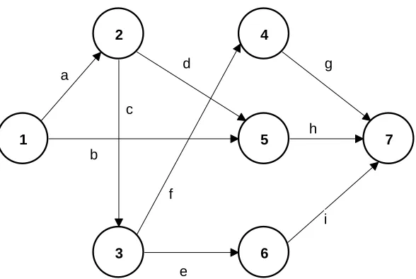
Figure 2. Sample project of 7 nodes and 9 activities solved via SPO ……… 47
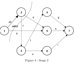
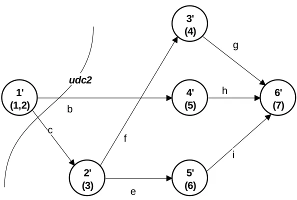
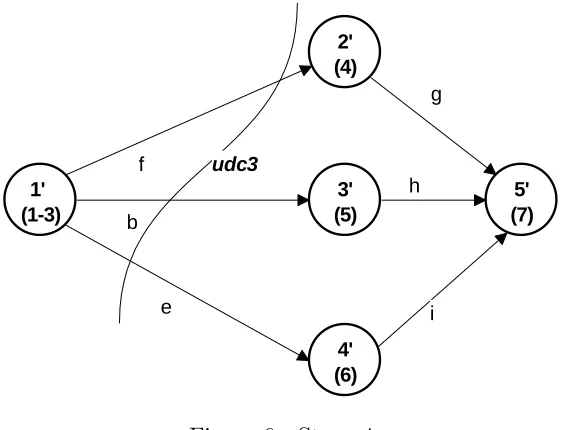
Figure 3. Sample project graph at stage 1 ……….…..……… 55
Figure 4. Sample project graph at stage 2 ……….…..……… 56
Figure 5. Sample project graph at stage 3 ……….…..……… 57
Figure 6. Sample project graph at stage 4 ……….…..……… 58
Figure 7. Sample project graph at stage 5 ……….…..……… 59
Figure 8. Sample project graph at stage 6 ……….…..……… 60
Figure 9. Sample project graph at stage 7 ……….…..……… 61
Figure 10. Sample project graph at stage 8 ……….…..……….. 62
LIST OF TABLES
1
Introduction and Motivations
1.1
Introduction
This thesis is concerned with the optimal allocation of resources to activities in projects in order to optimize an economic objective function. The latter is com-posed of the cost of the resources used and the penalty incurred (or reward accrued) if the project is completed later (earlier) than its promised delivery date. The context of our concern is projects in stochastic environments, where activities are related by ‘ordinary’precedence relations (as opposed to ‘generalized’precedence relations, see Elmaghraby and Kamburowski [7]) and require resources for their execution.
Project management, which we take to mean “project planning and control”, under stochastic conditions is a complex and challenging task. While it may be easy to simply ignore the inherent randomness in the process and appeal to deterministic methods of optimization, in doing so, one clearly risks committing several serious errors; the most common of which is the (sometimes) severe underestimation of the expected project cost and completion time as well as the misallocation of resources leading to sub-optimal outcomes.
The di¢ culty with analysis of stochastic activity networks (SAN’s) is that few purely analytical methods exist for optimization of such networks. Further adding to the di¢ culty is that the methods that do exist are tractable for only the smallest of problems. In order to be of practical utility for mid-size (50 to 150 activities) and large projects (over 150 activities), which is our concern, new methods must be developed, which is the subject matter of this thesis.
1.2
Motivations
clear that a project manger is primarily faced with a sequential (multi-stage) deci-sion problem –the manager’s world is a dynamic world in which favorable as well as adverse conditions may prevail, necessitating continuous adaptation to the new envi-ronment. A project starts with some resources, the resources are assigned, activities seize the resources for some random amount of time until they are complete, then the resources are released calling for a new decision on reallocation to the next set of activities. This process repeats until the project is completed.
The points of departure of this thesis from the conventional view of project plan-ning and control are two: (1) …rstly, thatmanagers manage resources, hence the de-cision variable is the amount of resource(s) allocated to each activity in the project. (2) secondly, thatuncertainty resides in the work-content of the activity not, as com-monly viewed, in its duration. The duration of the activity is the consequence of the resource(s) allocation, not its prime factor.
What would be useful is a ‘black box’ (BB) that takes in as input the current state of the project at a given stage (a point where a (re)allocation decision of the resource(s) is required) and outputs the optimal resource allocation decision based on the current state. In this way the problem may be viewed as a multi-stage control problem where the BB functions as the controller. The primary goal herein will be to propose a design for an e¤ective BB to solve this "What do I do now?" problem. This problem referred to as the ‘single stage’or ‘static’problem will be the subject of chapter 2.
to estimate the distribution of the project cost subject to a given control strategy. This problem referred to as the ‘multi-stage’or ‘dynamic’problem will be the subject of chapter 3.
1.3
Review of Literature
In some sense it is possible to view this thesis as work on a modi…ed version of the well studied ‘resource constrained project scheduling problem’(RCPSP). The RCPSP may be stated simply as the problem of ‘how to schedule the activities while respecting the precedence relations and the resource availability?’ For a comprehensive review of the gamut of problems under the rubric of RCPSP, the reader should see the books by Demeulemeester and Herroelen [5] and Neumann, Schwindt and Zimmermann [11]. As mentioned in the opening, the departure of our optic from the conventional view of project planning and control resides in two points, which we elaborate next.
First, our insistence that managers manage resources, not schedules and timeta-bles. In our view the project is a dynamic environment where many (or at least a few) opportunities will arise for the manger to intervene by reallocating resources. Hence the decision variable is the amount of resource(s) allocated to each activity in the project. The duration of an activity is the consequence of the resource(s) allocated to it, not its prime factor, as is commonly viewed. The intimate relationship between the resource allocation and the activity duration (and thus the project duration) was recognized early in the development of the …eld, see chapter 2 of the book by El-maghraby [8] for a comprehensive review of the early attempts at ‘time/cost trade-o¤ optimization’. We model time/cost trade-o¤ by using the concept of ‘work-content’ of an activity (more on this in §2.2) .
resource. The exact functional relationship will be discussed in detail in §2.2. The addition of this stochastic element gives rise to a stochastic optimization problem that is not trivial to solve (see §2.6). Our goal in chapter 2 will be to e¢ ciently solve this problem.
The literature dealing with stochastic optimization is quite broad and beyond the scope of this thesis, but we will brie‡y mention the methods we have explored in the course of our research.
Stochastic Approximation, a method originally introduced by Robbins and Monro [13] and later studied by Wolfowitz [17] was investigated but later abandoned because of its di¢ culty dealing with constraints. In particular Stochastic Approximation has trouble with the non-linear inequality constraints that are required in our model to enforce precedence relations among the activities. See §2.3 for a description of the model. Furthermore Stochastic Approximation, although possessing interesting theoretical convergence properties, did not perform well in practice even for simple examples of our model.
value at the rate O(1=pn) where n is the number of independent samples taken in the MCS. In order to make a reasonable comparison between two candidate solutions, the sample size must be su¢ ciently large to achieve acceptable convergence. What constitutes ‘acceptable’is a matter for the investigator to decide, but in our exam-ples it seemed thatn 200 was required, which led to unacceptably long computing times. Another problem with GA is that it lacks theoretical convergence properties, so it can be di¢ cult to determine stopping criteria.
In spite of these di¢ culties, Chu and Yao [3] proposed a GA methodology for the solution of the stochastic RCPSP which uses MCS. Later, Chu, Yao, and Tseng [4] proposed modi…cations to their original method that appear to increase computa-tional e¢ ciency by an order of magnitude. In both cases the graphs tested range from 11 to 22 activities and thus can be considered ‘small’by our classi…cation. To date no further results have been published exhibiting the application of their method on mid-size (50-150 arcs) or large (>150 arcs) size graphs.
Azeron, Perkgoz, and Sagawa [1] cast the problem as an optimal control problem which they readily admit can not be solved analytically. Instead, a GA is proposed for the solution of the apparently intractable control problem. As with the aforemen-tioned GA papers, the size of networks optimized by Azeron et. al. are smaller than 50 activities. Our goal is to solve mid-size and large networks, so GA was evaluated and deemed to be un…t for our purpose.
Dynamic Programming (DP) is yet another method that has been applied to the solution of the stochastic RCPSP. The reader may consult Tereso, Araujo, and El-maghraby [14],[15] for a concise description of the solution procedure via DP and the subsequent results using the procedure on a series of test networks. Although DP is elegant theoretically in the way it models the dynamic nature of the project manage-ment process, it su¤ers from severe problems computationally which are documanage-mented by the authors. For this reason DP is not practical for large projects.
alternate approach using the novel Electromagnetism Algorithm (EMA) optimization method of Birbil and Fang [2]. Using EMA they were able to get results far superior to the earlier DP results. For example they solved for the optimal resource allocation for a project of 76 (stochastic) activities in less than 8 hours using EMA, whereas with DP they were forced to abort their program after one week without obtaining results.
Based on our research, it would seem that the EMA approach is the ‘state of the art’for the stochastic RCPSP in that it is one of only two methods we came across that demonstrated actual numerical results for the optimization of stochastic projects with more than 50 activities. It is the sole method we found in the literature that reported computing times to achieve solutions as a measure of practical e¢ ciency. For these reasons we chose to use the EMA results as a benchmark for the performance of our proposed method. We compare our results with respect to both numerical accuracy and computational speed to the results of Tereso, Araujo, and Elmaghraby [16] in §2.9.
Based on our research we decided that Sample Path Optimization (SPO) was the most promising choice for the solution of the stochastic RCPSP. For a comprehensive review of SPO see Gurkan, Ozge, and Robinson [10] . Our interest in SPO was originally sparked by an insightful paper by Plambeck et al [12] in which the method of SPO was applied to solve the stochastic RCPSP. In their paper, networks of up to 110 activities were solved; however no results were published indicating the computing time required to achieve solutions. We suspect that the results in their paper would have served as a good benchmark (along with the EMA method mentioned above), but there are several material di¤erences between our model and Plambeck’s that make such comparison di¢ cult.
of the underlying (activity duration) distributions. Because of the terms of the form
kizi 1 in their objective function, there is the desired time/cost trade-o¤. In contrast,
our model uses an objective which is the expected value of a cost function, where the decision variables are kept separate from the parameters of the underlying (work-content) distributions. Section 2.2 will discuss our cost function in detail and give our rationale for choosing to model time/cost trade-o¤ in this manner.
A second di¤erence in Plambeck et al’s model is that they specify either triangular or uniform distributions to represent the durations of the activities. In the case where uniform distributions are used, the mean of the activity duration zi is taken
as the decision variable for activity i. The assumption is that the expected duration of an activity may be perturbed at some cost, however there is nothing that can be done about the variance. In the case of triangular distributions, the authors suggest a common scaling factor for the minimum, the maximum, and the mode of each activity duration distribution. In other words, activity i has a duration that is randomly distributed as a triangular distribution with parameters azi; bzi; czi where
the common factorzi is the decision variable anda; b; care the minimum, mode, and
maximum; respectively. The use of the triangular distribution in this fashion allows the expected duration and the variance to be perturbed at some cost. In contrast our model allows for the use of any distribution to represent work-content (see §2.10 for a more detailed discussion of this aspect), and because our distribution parameters are not imbedded in the objective as decision variables, we have more freedom to modify our cost function as needed without requiring a speci…c form for the input distributions.
not able to use the results of Plambeck et al as a direct benchmark for our method, the paper was of signi…cant interest to our problem, because it motivated the seed that eventually grew into our solution procedure.
An outline for the main body of this thesis is as follows: Chapter 2 de…nes the single stage (static) problem in §2.1. The particular model of the RCPSP that we used will be discussed in both its deterministic (§2.3) and stochastic (§2.6) forms along with a discussion of the cost function (§2.2). In §2.7 we will review the basics of SPO then apply the method to the solution of our SAN problem in §2.8. Chapter 2 will conclude with a comparison of the results achieved using both SPO and EMA on the same test project (§2.9), and …nally conclusions and suggestions for future research (§2.10).
Chapter 3 opens with a discussion of the multi-stage (dynamic) problem and suggests a procedure for analyzing the problem using MCS in §3.1 . Section 3.2 discusses some methods for bounding the optimal expected cost of the multi-stage problem using Jensen’s inequality to …nd a lower bound, and the single stage solution via SPO to …nd an upper bound. A numerical example of the MCS procedure from §3.1 is presented in §3.3. Finally Chapter 3 concludes with summary and directions for future research in this area; §3.4.
1.4
Project Representation and Notation
and terminal nodes written as an ordered pair such as(i; j). Thestart node (source) of the entire project will always be designated as node1 and theterminal node (sink) as noden, where n is the largest numbered node in the set N. A node is considered to be realized (or activated) when all of the activities terminating in the node have completed processing. At the time of realization of a node, all activities emanating from it may begin immediately and are referred to as ‘sequence-feasible’(sf) activities. By convention, the realization time of node1 is taken to be zero and the realization time of noden represents the makespan (total duration) of the project.
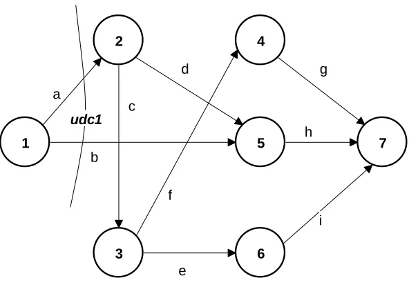
Before beginning chapter 2 we have to introduce one more concept, that of a ‘uniformly directed cutset’(udc). As the name indicates, it is a ‘cutset’that partitions the set of nodes in the graph into two subsets, call them V and V = N V; such that the start node1 is inV and the terminal noden inV ; with the property that all the arrows in the cutset are in the direction from V into V’. Theudc’s of a graph represent sets of activities that can possibly occur simultaneously (in parallel). We will denote the udcs of a graph by C1; C2; :::; Ck with C1 always designated as the
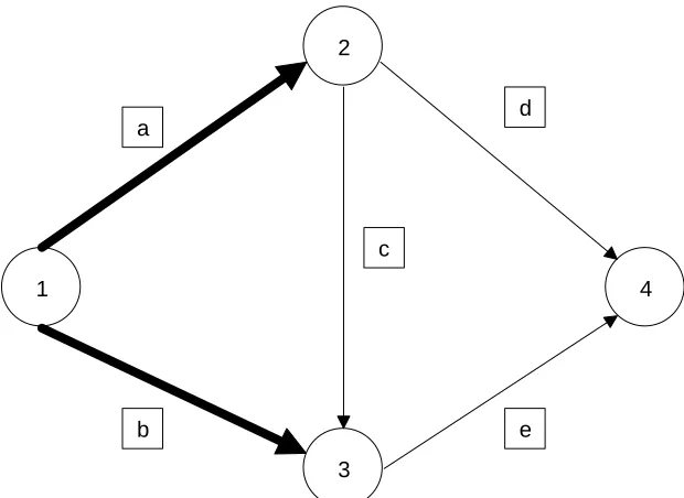
startingudc (the set of activities emanating from node1). Example 1 below gives the parameters of a simple graph that is displayed in Figure 1 (the so-called ‘interdictive graph’). In this graph the activities in the …rst udc are highlighted in boldface since they play an important role in the mathematical model to be developed; see §2.3 below.
Example 1 (the IG):
N = {1,2,3,4}
M = 2 6 6 6 6 6 6 6 6 6 4 1 2 1 3 2 3 2 4 3 4 3 7 7 7 7 7 7 7 7 7 5 1 2 3 4 d c b a e
In addition to the graphG ,we need to de…ne the following vectors, all of which are indexed on the set A:
r : resource costs per unit
W : work-contents (a random possibly correlated vector)
w : work-contents (a particular random sample ofW or a constant vector )
x : resource allocations (the decision variables)
d : activity durations : lower bounds on x
: upper bounds onx s : start times
f : completion times
Other parameters of the project are:
[W] : sample path matrix where each row is an independent sample ofW T : due date of the project
: cost of tardiness per unit time
ti : realization time of nodei
KT: portion of project cost due to tardiness
KR: portion of project cost due to resource requirements K: total project cost KR+KT
Kn : sample mean project cost derived from a sample of sizen
2
The Single Stage Stochastic RCPSP
2.1
De…nition and Discussion
A project manager is faced with a sequential (multi-stage) decision problem. In order to analyze the multi-stage process, we begin by breaking it down into its constituent parts (single stages) and determine how to optimize these stages individually. How to analyze the multi-stage (or dynamic) problem as a whole will be considered in chapter 3. In this chapter our concern will be to propose a ‘black box’(BB) solution procedure that can determine the optimal static policy that should be followed for a given stage. By ‘stage’ we mean a point in time at which a resource allocation decision is required by the manager. In order for the BB to function, it must be provided with the necessary information to completely de…ne the state of the project at the beginning of the stage in question. In our case the information that is required is the project graph and all of its parameters (precedence relationships, activity work-content distributions, etc. ). Given this information, the BB calculates the optimal resource allocation vector x 2 X RjAj which is the optimal static policy to be carried out throughout the project. In other words, the resource(s) will be assigned to the set of activities and remain static in the sense that no future reallocations of resource will be permitted. Therefore there is only one decision for the manager to make at the onset of the project, then he/she becomes an observer locked into the allocations made at time zero. Thus the optimal static policy may be stated as the vector of resource allocations x that results in the minimum expected project cost
K under the static conditions described above.
processing at the time when the resource allocation decision is made. In large projects it will usually be the case that the set of starting activities (those activities that may begin at time zero) will be very small when compared to the number of total activities in the project. This is like forcing a tennis player to specify right now the exact position on the court where his/her feet will be to return serve for some future point. Obviously it is possible to hazard a guess as to where your feet should be based on facts you know about the strategy of your opponent, but a skilled player places themselves in a likely position, then reacts and adapts at the actual moment when the ball is served. The same is true of a skilled project manager who tentatively earmarks resource allocations for future activities and then waits to see how the uncertainty of the project manifests itself before adaptively choosing the …nal allocation. In large projects with many uncertain events it will almost always be the case that the tentative guess made at the start of the project will not match up with the actual allocation that is eventually made.
project is just a single activity. The mechanisms for transition from one stage to the next and updating the state variables (project parameters) will be discussed in chapter 3, but for now we wish to propose a method that solves the single stage (static) problem optimally. We will install this procedure as our BB when we analyze the multi-stage (dynamic) problem later in chapter 3. We begin chapter 2 by introducing the concept of ‘work-content’in the context of our basic model for resource cost.
2.2
Work-Content, Activity Duration, and Resource Cost
We begin our analysis of the resource cost function with the obvious question: what is work-content? Just from looking at the name, one could guess that work-content is a property of an activity that somehow measures the amount of ‘work’the activity requires. In our context ‘work’is a quantity measured in units of resource times units of duration (e.g. man-hours). From previous discussions we know that there must be a functional relationship between work-contentw(i;j), duration d(i;j), and resource
allocationx(i;j) for each activity (i; j)2A . In addition we know that as the resource
allocation is increased, the duration of the activity decreases (within certain bounds). Therefore we may take the following as a general model for this relationship (dropping the subscripts),
d = w
xk
Rewriting the terms and taking 0< k 1gives:
w=dxk
Based on the analysis above there will be an in…nite number of modes of execution for an activity (x is assumed to be continuous), but we know that for every mode (x; d); the product dxk is always equal to the constant w. This fact suggests that if the project manager can give us just one mode of execution, then the work content
w is de…ned across all modes of execution.
The …rst assumption we make is that a manager can determine a priori for a particular activity (i; j)2A how the allocation x(i;j) should be bounded from above
and below. In other words the manager knows how to de…ne an interval (i;j); (i;j)
of the values that x(i;j) can assume. We claim that somewhere on this interval there
exists an allocation xm that will be referred to as the ‘neutral’ resource allocation
for activity(i; j). We de…ne ‘neutral’as the situation where there is neither pressure to crash the activity by allocating maximum resource (x(i;j) = (i;j)) nor lag in the
execution of the activity by applying minimal resource (x(i;j) = (i;j));instead we are
faced with the ‘usual’or ‘neutral’situation. Assume that the manager can provide us with the mode(xm; dm)corresponding to an allocationxm that is considered ‘neutral’.
We further assume that the experienced manager can determine the duration dm of
an activity given that the ‘neutral’ level of resource xm is applied. Since we have
taken w as a constant, it may be expressed in terms of the ‘neutral’ mode by the following:
w=dmxkm
level (in the opinion of the contractor) that will get the job done at a reasonable, but not extreme pace. Therefore the ‘neutral’mode of execution is given by (xm = 2
machines, dm = 5 days) and the work-content w = 10 machine days (we let the
parameter k= 1 for this example).
Next we turn our attention to the resource cost cR given on a per time unit
of duration basis. We model the resource cost cR as an increasing function of the
resource allocation x:
cR=rxp; p > 0
Putting everything together we de…ne the total resource cost KR incurred to
complete a particular activity by the following:
KR=cRd= (rxp)d=rwxp k =rdmxkmx p k
The DAN model that will be presented in §2.3 uses k = 1 and p= 2 re‡ecting a hyperbolic relationship between duration and allocation (w = dx), and a quadratic relationship between cost and allocation (cR =rx2). In general we require thatp > k,
because we desire KR to be an increasing function of the allocation x. Consider the
following example:
Example 2 w= 10 man-hours, k = 0:5; p= 2; and r= 1: x d= p10
x cR =x
2 KR =cRd
1 10 1 10
2 7.07 4 28.28
3 5.77 9 51.96
4 5 16 80
returns would be this dramatic in practice, but it gives the general idea. It can be seen
that ‘crashing’this activity (allocating maximum resource) gets the job done twice as
fast (5 hours vs. 10 hours) at a total cost that is eight times greater ($10 vs. $80). An
activity that has a similar resource cost function would have to pay a high premium
to reduce duration and thus could become very costly if it lies on the critical path in
the deterministic case or has high likelihood of being on the critical path (criticality
index near 1) in the stochastic case.
2.3
The Deterministic Activity Network Model (DAN)
In the deterministic case, the work-content vectorwis known with certainty. The de-cision facing the manager is how to allocate resources among the competing activities in such a way as to minimize the total cost of the project. Our model assumes that there is a single in…nitely divisible resource required by all activities (e.g. man-hours). This model can be easily enriched by the addition of more resources (e.g. trucks and man-hours), with appropriate changes in the constraining relations, but for the sake of simplicity we initially consider one resource only . The supply of the resource is limited and the permissible allocation to each activity is bounded from above and below. The project has no …nancial incentive for …nishing before the due date T, however a cost of is incurred per time unit of tardiness. The cost of resource uti-lization for a particular activity (i; j)2A is assumed to be quadratic in the amount of the resource allocation for the duration of the activity, KR x2(i;j); with the
con-stant of proportionality denoted by r(i;j), per unit per unit time of duration of the
activity. Let the latter (the activity duration) be denoted by d(i;j). The duration of
an activity also must be a function of the resource allocation. Obviously the resource cost for a particular activity is an increasing function of its allocated resource. To model time/cost trade-o¤ a method must be adopted to relate the duration and the allocation. For simplicity assume d(i;j) = w(i;j)x(i;j1) 8(i; j) 2 A. This choice is not
half, but it is a reasonable approximation provided that the bounds on the allocations are not too loose. Thus the resource costKR of activity(i; j)with work contentw(i;j)
and resource allocation x(i;j) may be stated as
KR =r(i;j)x2(i;j)
w(i;j)
x(i;j)
=r(i;j)x(i;j)w(i;j):
It can be seen that the particular form of KR we have selected results in a linear
function inwfor any …xedx. This model can also be easily extended to more realistic resource-duration functional relations, such asd=w=pxwhich implies that doubling the resource allocation would reduce the duration by only1=p2'0:7instead of 0.5. This would render the model more realistic, but would complicate the analysis with little addition in insight.
To complete the project cost functionK(x; w) =KR+KT, we de…ne the tardiness
cost KT by the following:
KT = max (0; tn T)
This function re‡ects our model which incurs a cost of per unit time if the project …nishes past the due date T (i.e. tn T > 0), but o¤ers no …nancial incentive for
early completion of the project .
This structure motivates the following optimization problem which shall be re-ferred to as the ‘deterministic activity network’(DAN) problem:
min
x K(x; w) =
X
(i;j)2A
r(i;j)w(i;j)x(i;j)+ max (0; tn T); (1)
s.t.
ti tj +w(i;j)x(i;j1) 0 (2)
X
a2C1
xa R; (4)
8(i; j)2A; all variables non-negative: (5) Equivalently, by replacing the ‘max’ function with a new variable y and adding constraints
y tn T; y 0 (6)
the objective function changes to
min
x K(x; w) =
X
(i;j)2A
r(i;j)w(i;j)x(i;j)+ y; (7)
s.t. constraints (2)-(6).
In the DAN model presented above, we have a total jAj+jNj variables. For the sake of exposition, we separate the variables into 3 groups: decision, temporal, and tardiness. There is a decision variable x(i;j) corresponding to the resource allocation
to activity(i; j). There is a temporal variableti corresponding to the realization time
of each nodei = 2;3; : : : ;jNj (node 1 is omitted because it is assumed to be realized at time zero). In addition there is a single variable y that represents the tardiness. The variables are categorized using this nomenclature to stress that resource decisions made by the manager result in temporal and tardiness consequences. It is important to realize that in seeking the optimal solution to this DAN model there arejAj+jNj
structural variables (not just jAj for ‘decision’variables).
Focusing on the objective function, it can be seen that there are two separate cost components. The summation term
KR = X
(i;j)2A
r(i;j)w(i;j)x(i;j)
The …nal term in the objective function represents the cost due to tardinessKT = y. If the project …nishes early or on-time, the tardiness cost will be zero, otherwise the tardiness cost is a linear function of the tardiness L = tn T. Many other
possible objectives exist such as minimizing project makespan tn or maximizing the
NPV (net present value) of the project cash ‡ows, but the focus of this thesis will be the objective of cost minimization.
The constraints can be divided into four categories: temporal, tardiness, aggregate resource, and ‘box’constraints. There is a temporal constraint associated with each activity (i; j)2A of the form ti tj +w(i;j)x(i;j1) 0. Temporal constraints ensure
that the precedence structure de…ned by the graph G is respected. To see why this is true, notice that a temporal constraint may be rewritten as tj ti d(i;j) which
indicates that the time elapsed between the node realization times of the start and terminal nodes of activity(i; j) must be at least as large as its duration. The single tardiness constraint: y tn T is required to replace the nonlinear ‘max’function
in the …rst version of the objective function. This gives the desired result of a non-negative linear tardiness cost function. The ‘box’ type constraints are upper and lower bounds on the resource allocation vector x. The aggregate resource constraint P
a2C1xa Rrestricts the combined resource allocated to the activities in the starting
udc C1 to no more than the total amount of resource available R. It is important to
of resource R: If R is large, then there will be very little di¤erence, but if R is relatively small the di¤erence can be signi…cant. In this thesis we temporarily avoid this problem by assuming thatRwill be set su¢ ciently large to ensure that the lower bound on optimal cost produced by the DAN model is a good approximation of the true optimal cost under the assumption of …nite resource availability. Dealing with the problem directly is a topic of on-going research that will be dealt with in future papers.
2.4
A Geometric Programming Model (GP)
The mathematical program presented for the DAN is a non-linear program (NLP). It may be solved with varying degrees of accuracy by many commercially available solvers. However there are several problems involved with using general NLP routines to solve the DAN optimization problem. The highly non-linear structure of the problem can lead to poor performance for Newton type NLP routines (bogging down in steep valleys or very ‡at plateaus). Secondly, for large problems involving hundreds of activities, NLP routines run unacceptably slow. As will be discussed later in §2.8, we are usually interested in solving not just the DAN optimization problem, but a much larger related problem which we label EDAN. It is therefore a must that an extremely e¢ cient method for solving the DAN problem be selected. Thirdly, almost all NLP routines known to us are sensitive to the ‘seed solution’–change the initial point of iteration and you may get a di¤erent result –so that one is never sure that the solution in hand is the true global optimum.
The DAN problem stated above can be transformed into a standard GP form by some elementary algebraic manipulations applied to the original DAN model. The goal is to get the objective function and all the constraints to be the sum of posynomial terms (i.e., each is of the form a j x
nj
j ; a > 0; nj rational for all j), and all the
constraints of the form 1: After applying the required algebraic manipulations we have the GP standard form of the DAN model given by the following:
min
x K(x; w) =
X
(i;j)2A
r(i;j)w(i;j)x(i;j)+ y+ (a constant) (8)
s.t.
titj1+w(i;j)x(i;j1)tj1 1 (9)
tny 1 1 (10)
T y 1 1 (11)
1
(i;j)x(i;j) 1 (12)
(i;j)x(i;j1) 1 (13)
1
KR
X
a2C(1)
xa 1 (14)
8(i; j) 2 A and 82 i < j n; t1 = 0; (15)
all variables strictly > 0: (16)
the optimum and must be accounted for eventually. It is the result of the following necessary conversion:
max(tn T;0) = [max(tn; T) T] = max(tn; T) T
) y T
given that y tn and y T. Such a conversion was required because the original
form calls for a constraint y tn T which is not possible to get into the required
posynomial 1form.
The …nal GP form is obtained by a logarithmic change of variables; put
z(i;j) = ln(x(i;j)) ; 8(i; j)2A
zy = ln(y)
qv = ln(tv) ; 8(v)2N f1g:
Substitution in the GP model above yields:
min
z K(z; w) =
X
(i;j)2A
r(i;j)w(i;j) exp(z(i;j)) + exp(zy) + (a constant) (17)
s.t.
exp(qi) exp(qj) 1+w(i;j)exp(z(i;j)) 1exp(qj) 1 1 (18)
exp(qn) exp(zy) 1 1 (19)
Texp(zy) 1 1 (20)
1
(i;j)exp(z(i;j)) 1 (21)
1
KR
X
a2C(1)
exp (za) 1 (23)
8(i; j)2A: (24)
The model of (17)-(24) is the model used in the implementation detailed in §2.5 below. The solver chosen to run the experiments is ‘Mosek’ (www.mosek.com), a commercially available solver that interfaces seamlessly with Matlab. The GP algo-rithms employed by Mosek are based on interior point methods closely resembling those used with great success to solve linear programs.
2.5
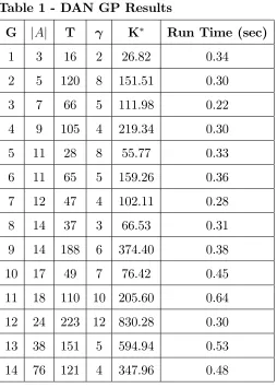
DAN Experimental Results
The GP model detailed in §2.4 was implemented on 14 networks of varying num-ber of activities ranging between 3 and 76 activities. The detailed speci…cations of the networks are given in Appendix B. Our eventual goal is to handle stochastic work-contents, however we begin with the deterministic case …rst, then extend the methodology to the stochastic case. Therefore initially we consider these 14 graphs as having known work-contents given along the row designated as “mu”. Later in §2.9 when we experiment with these graphs as stochastic projects this row in Appendix B will give the mean = 1= for the exponentially distributed work-contents. The resource cost r(i;j) was normalized at one 8(i; j) 2 A for all projects. The due date
Table 1 - DAN GP Results
G jAj T K Run Time (sec)
1 3 16 2 26.82 0.34
2 5 120 8 151.51 0.30
3 7 66 5 111.98 0.22
4 9 105 4 219.34 0.30
5 11 28 8 55.77 0.33
6 11 65 5 159.26 0.36
7 12 47 4 102.11 0.28
8 14 37 3 66.53 0.31
9 14 188 6 374.40 0.38
10 17 49 7 76.42 0.45
11 18 110 10 205.60 0.64 12 24 223 12 830.28 0.30 13 38 151 5 594.94 0.53 14 76 121 4 347.96 0.48
2.6
The Stochastic Activity Network Model (SAN)
Our ultimate goal is to solve the stochastic optimization problem given by (25) be-low. Note that from this point forward we will refer to our version of the stochastic RCPSP as the ‘stochastic activity network’problem or the ‘SAN’problem. The main di¤erence between the SAN and DAN problems resides in the recognition that the work content of activity(i; j)is a r.v., denoted byW(i;j):The formal statement of the
min
x EW [K(x; W)] = EW[
X
(i;j)2A
r(i;j)W(i;j)x(i;j)+ max (0; n(x; W) T)]; (25)
s.t.
(i;j) x(i;j) (i;j) X
a2C1
xa R
8(i; j) 2 A
all the variables are non-negative.
in whichW is the random work-content vector, nis the project makespan (a function
of W; hence a r.v.).
Stated in words, we wish to minimize the expected value of the cost function
K(x; W) subject to the bounding constraints on the resource allocation x and an aggregate resource constraint placed on the starting udc C1: The random nature
of the cost function K(x; W) is a consequence of its dependence on the randomly distributed work-contents of the activities W. In addition the project makespan n
is itself also a r.v. that depends on both the allocation x and the random work content W. The expression for the tardiness cost KT = max (0; n(x; W) T)
via the method of Sample Path Optimization (SPO), which we brie‡y introduce in the next section. Note that our explanation of SPO is paraphrased from [10] (adopting similar notation).
2.7
Sample Path Optimization (SPO)
A general model for many problems in the area of stochastic (or simulation) opti-mization is as follows: we have an extended real-valued stochastic processfZn jn=
1;2; :::g, where the Zn are random variables (functions) depending on parameters
2Rk. For eachnand each ;we have a random variableZ
n( )de…ned on the
prob-ability space ( ;F; P) which may take either real values or the value +1: When a particular sample! 2 is …xed, we writeZn(!; )to indicate the dependence on the
…xed sample !.
In certain stochastic optimization problems, we have a priori knowledge that there exists a deterministic function Z1( ) such that the functions Zn almost surely
converge point-wise to Z1 as n ! 1. For example in the case of a static system like our SAN problem, the strong law of large numbers ensures convergence when Zn
is the average ofn independent replications (project cost realizations). In the case of dynamic systems such as queues, if we take Zn as the output of a simulation run of
lengthn (e.g., nservice completions), the existence of Z1 can often be inferred from regeneration theorems. In this thesis we will deal strictly with the optimization of SAN’s via Monte Carlo sampling (MCS) and therefore can be certain thatZ1exists. In particular we are interested in …nding the in…mum of Z1 and, if possible, a value of at which the in…mum is achieved (a minimizer of Z1).
Then indeed we should have solved the problem posed.
In general it will be the case that we cannot observe Z1; but instead we have to be content with the estimator Zn( ) for a given (…nite) n and particular : We
will use observations ofZn( )to approximate the minimizer and minimum value that
we are seeking. The method under consideration, namely Sample Path Optimization (SPO), is described simply as follows. We …x n and take a sample ! of size n, then we apply deterministic optimization methods to determine the minimizer n of the
(deterministic) function Zn(!; ). We will assume that this minimizer exists in our
application to SAN’s, however the reader should see [10] for a discussion of conditions under which the minimizer exists. We simply take nas an estimate of the minimizer of Z1. SPO is very attractive because, in many cases, very powerful methods (in particular, GP) can be applied to minimizeZn(!; ), even when numerous complicated
constraints on are present. Applied to our concern, n is ourxn which will serve as
the estimate of ; and Z1 is our EW[K(x; W)]:
2.8
SPO Applied to the SAN Problem
SPO is applied to the solution of the SAN problem by observing the following: In our case the stochastic process under consideration is a series of sample mean project costs fKn(x)jn = 1;2; :::g derived for a particular resource allocation x2X RjAj
for a sample size n. The sample mean project cost Kn(x) for a given allocation x
and sample size n may be expressed as follows:
Kn(x; w1; w2; : : : ; wn) =
1
n n
X
i=1
K(x; wi)
Where w1; w2; : : : ; wn (vectors) represent a series of n independently and
lim
n!1
1
n n
X
i=1
K(x; wi) =EW[K(x; W)]
This result implies that we may use SPO to approximate the optimal solution to the SAN problem presented in §2.6. The quality of the approximation improves as the sample sizen ! 1. An interesting question which shall be dealt with presently is how small cann be and still achieve ‘close enough’results?
When the number of samples (project realizations) is …xed at size n ( 1), we refer to the set ofn project realizations as a ‘sample-path’of length n. To make our notation more compact we shall compose a sample path matrix[W]using the vectors
w1; w2; : : : ; wn row-wise. Since each project realization wi is a sample of the vector W; wi will have jAj elements. Therefore our sample path is a matrix [W] comprised
of n rows and jAj columns where each row represents an independent sample ofW. In order to use SPO to solve the SAN problem, we must …rst construct a determin-istic function Kn(x;[W]), that utilizes the sample path information (now constant
matrix [W]) and has as its domain the feasible decision space of resource allocations
X RjAj\(bounds). Furthermore the function Kn(x;[W]) will almost surely
con-verge point-wise toEW[K(x; W)]asn! 1 where the notationEW means taking the
expected value of the random project cost function K(x; W) by integrating over the sample space of the random work content vectorW. As mentioned previously, if we chooseKn(x;[W])to be the sample mean project cost over thenindependent project
realizations, then by invoking the strong law of large numbers, the requirements for SPO are met.
that produces the minimum costK for a particular realizationwof the project. Our goal in using SPO is to …nd a minimizer that produces the minimum cost ‘on average’ when that allocation is implemented to all possible realizations of the project.
In order to accomplish this objective, we extend the DAN model through the addition of new variables and constraints. This ‘extended’model will be referred to as the ‘extended deterministic activity network’ or EDAN for short. We desire the optimizer x that produces the minimal average cost over all possible realizations of the project. Of course we can not test an in…nite number of realizations to evaluate the quality of a given candidate solutionx2X (recall that we had assumed the work contentW(i;j) to be a continuous r.v. , but even when it is a discrete r.v. the number
of combinations are usually too large to enumerate). So, instead, we determine the optimal allocation for a sample of sizen, and denote it byex:We maintain thatxeis an approximation to x , and that the approximation improves asn increases so that in the limitxe!x :Our sample path[W]representsn independent project realizations, so our functionKn(x;[W])is calculated by summing upnproject costs (and dividing
the sum by n) where each individual cost is derived using the allocation x and the row of [W] corresponding to the realization in question.
Continuing toward our goal we must construct a mathematical program that min-imizes the approximating function Kn(x;[W]) subject to constraints ensuring that
the precedence structure de…ned by the project graph G is respected independently for each sample (realization). Recall that the sample path[W](and thus the function
Kn(x;[W]) ) is composed of n independent samples of the work-content vector W.
Since every sample can (and usually will) be di¤erent, the activity durations which depend on the work-contents will also vary for di¤erent realizations. In turn, the node realization timesfti :i2Ngand tardinessywill also di¤er. Therefore a separate set
therth row (r = 1;2; :::; n)of the sample path matrix [W] ast(r)
i : In addition denote
the tardiness incurred in realization r as y(r) = max
f0; t(nr) T g and [W]((ri;j)) as the
element of the sample path matrix contained at the rth row , activity(i; j) column.
We now have the necessary information to write our objective explicitly:
min
x2X K(x;[W]) =
1
n n
X
r=1 X
(i;j)2A
r(i;j) [W] (r)
(i;j)x(i;j)+ y (r);
in which the space of feasible decision vectorx is speci…ed by the constraints on the individual activity allocations.
min
x2XK(x;[W]) =
1
n n
X
r=1 X
(i;j)2A
r((ri;j)) [W]((ri;j))x(i;j)+ y(r);
s.t.
t(ir) t(jr)+ [W]((ri;j))x(i;j1) 0
y(r) t(nr) T
(i;j) x(i;j) (i;j) X
a2C1
xa R
8(i; j) 2 A; r = 1;2; :::; n;
and all variables non-negative.
We denote by ex(i;j) the optimal resource allocation to activity (i; j) derived from
the above model.
As in the case of the DAN problem, the constraints for the EDAN can be divided into four categories: temporal, tardiness, aggregate resource, and ‘box’ constraints. There is a temporal constraint associated with each activity (i; j) under realization
r of the form t(ir) t(jr) + [W]((ri;j))x(i;j1) 0. Temporal constraints ensure that the precedence structure de…ned by the graph G is respected independently in each realization. There is a single tardiness constraint: y(r) t(nr) T for each realizationr
that is required to replace the functionmaxf0; t(nr) T gused to model the tardiness as
a non-negative linear function. Since we are minimizing over the resource allocation vector x; which will be applied to all realizations identically, we require only one aggregate resource constraint on the starting udc C1 and a single set of jAj upper
The use of the term ‘extended’ to describe the program should now be clear. Notice that the number of variables and constraints have been increased for the EDAN as compared to the DAN. The number of variables has been expanded from jAj+jNj for the DAN to jAj+njNj variables for the EDAN. In a similar fashion, the number of temporal constraints has increased from jAj for the DAN to njAj for the EDAN, and the number of tardiness constraints for the EDAN is n whereas the DAN used only one. The common thread here is that the size of the program has been extended by roughly a factor of n due to the fact that the EDAN considers n
project realizations simultaneously as opposed to just one.
Like the DAN model, the EDAN model will be formulated and solved as a geo-metric program. See §2.4 for the rationale behind this choice and the procedure for converting the model to a GP standard form.
The question now becomes just how large does n have to be until ‘closeness’to the exact value is reached? In other words how fast does the sample mean cost (and sample optimal policy) approach the true expected project cost (and exact optimal allocation vector)? The answer is of course problem speci…c, but if acceptable con-vergence can be achieved for a reasonably small value ofn (say less than 1000), then the EDAN may be converted into a GP that can be solved globally in an acceptable amount of time.
A simple procedure for determining if n is appropriately large is to generate a series ofm independent sample paths f[W]1;[W]2; ::;[W]mg each of sizen rows. For each of themsample paths solve the EDAN problem resulting in a data set of optimal sample mean costsKs=fK1; K2; ::; Kmg. Calculate the sample meanbK and sample
standard deviationsK for the datasetKs:Finally compute the coe¢ cient of variation
for the data set cvK = sK=bK: If cvK < " where " is a tolerance speci…ed by the
2.9
SPO Results and Comparison to EMA
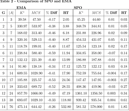
The spreadsheet in Appendix B gives the speci…cations for a series of 14 test projects that we optimized via SPO. Since we are now viewing these graphs as stochastic projects, the row in the spreadsheet labeled "mu" gives the mean = 1= for the exponentially distributed work-contents of each activity. In this section we focus on the (largest) project of 76 activities labeled ‘Graph 14’in Appendix B. This project was originally studied by Tereso et. al. [15] in their paper using EMA. In the section below we compare our results using SPO for Graph 14 to the results reported using EMA on the same project.
Examination of Appendix B (Graph 14) reveals that the results obtained using our SPO procedure di¤er from those obtained through the use of EMA for the same project (see the summary data at the very bottom of the sheet). In particular the optimal expected cost for EMA is reported as 475:14; compared to 581:52 for SPO. We also observe a di¤erence in the optimal resource allocations nx(i;j)o where the optimal allocations for EMA are almost always smaller than the corresponding opti-mal allocations for SPO. Since the optiopti-mal expected cost for EMA is sopti-maller and the optimal solutions di¤er considerably, we certainly can not claim that both SPO and EMA are appropriate optimizing approaches, and further validation of the results are required.
is very di¢ cult to demonstrate through numerical experimentation that x is the optimizer, it is relatively easy to check by MCS whether or not the adoption of the static policy x actually results in a mean cost of K . The application of MCS to carry out this check is simple: we …x the allocation at x , then take a sample path of project realizations[W] of very long length (n 50;000) and simply evaluate the sample mean cost K using x and [W] (call the resulting evaluation KM CS). Thus
we have KM CS = K(x ;[W] ) where the function K is de…ned as in §2.8. If there
is a signi…cant di¤erence betweenKM CS and the reported optimal expected cost K
then it becomes very di¢ cult to claim optimality (in value) without …rst being able to claim accuracy (in allocation). In other words, how can an optimization procedure possibly iterate to the optimal allocation if it is not able to evaluate the quality of each candidate solution along the way accurately?
respective problems are roughly the same; so it seems reasonable to conclude that SPO is more e¢ cient than EMA while also being more accurate. To reinforce this conclusion we carried out the same analysis on all 14 graphs tested by Tereso et. al. [15]. The results appear in Table 2 below. Note that for the SPO experiments summarized in Table 2 we required cvK 0:03 for all projects tested (see §2.8 for
explanation). The due dates (T) and tardiness costs ( ) for each graph are given in Table 1 from §2.6.
Table 2 - Comparison of SPO and EMA
EMA SPO
G jAj K M CS % Di¤ RT K M CS % Di¤ RT
2.10
Conclusions and Areas for Future Research
Our goal in this chapter was to propose a method that e¢ ciently solves the single stage stochastic RCPSP. From the research we have conducted, it appears that SPO accomplishes this goal quite well. To conclude this chapter we shall summarize the contributions made by our analysis and also point out some areas of future research The ‘single stage’or ‘static’problem has been solved to a high degree of accuracy in a very e¢ cient manner using GP. To our knowledge there is no published work where GP has been applied to the optimization of activity networks. Furthermore a method (SPO) has been utilized that possesses theoretical convergence properties indicating that as the lengthn of the sample path[W]approaches in…nity, the optimal solution to the EDAN program (§2.8) approaches the optimal solution to the SAN problem (§2.6). The SPO method (implemented through the EDAN) has been formulated as a GP to bolster computational e¢ ciency and ensure unambiguous global optimality. Another signi…cant achievement that is unprecedented in the literature is the ability of the SPO method to e¢ ciently optimize stochastic networks in the hundreds (and possibly even thousands) of activities. As mentioned previously in the review of literature (§1.3), the largest successfully solved project that we encountered in our research of the stochastic RCPSP was the 110 activity graph solved in Plambeck et. al. [12]. In the course of our experiments, we have successfully optimized graphs with up to 1000 stochastic arcs. The results obtained from SPO experiments on stochastic graphs of 250, 500, and 1000 activities respectively can be obtained from the author by request (in spreadsheet format).
speci…ed by the user. As long as the speci…cation for W allows for random sampling via MCS, it is permissible. Therefore W is free to be continuous, discrete, mixed, empirical, and even correlated, provided that we know how to randomly sample it and can easily determine the probability distribution of any ‘residual work-content’. (Recall that the assumption of exponentially distributed work content rendered this latter caveat unnecessary, thanks to the ‘memory-less’ property of the exponential distribution.) The problem of calculating residual work-contents only becomes an issue in the muti-stage case (see chapter 3), therefore the single stage problem de-scribed in chapter 2 is unfettered by this concern. In order for this ‡exibility in the form ofW to be possible, we have intentionally separated the parameters of the input distributions from the objective function. In other words the decision variables (the allocation vectorx) in the cost function are unrelated to the parameters of W (e.g,. mean, variance, etc.).
Another nice feature of our model is the output data it produces. In addition to producing the optimal allocation x and associated minimum average cost K , the optimal structural variables solution for the EDAN program also provides sample data for the optimal realization times of all the nodes of the project nt(ir)o
r=1::n ; i 2 f2;3; :::;jNjg, the optimal tardiness amount y(r)
r=1::n , and its cost. Using
this data, output analysis can be carried out to estimate the distributions of the makespan n; as well as every node realization time i : i 2 f2;3; :::;jNj 1g under
the optimal static policy x . The complicated random expression for tardinessKT =
max (0; n(x; W) T) may be analyzed using the output data supplied by the
EDAN. Therefore it is possible to investigate the relative importance of the tardiness cost versus resource cost for a particular project.
be taken as any posynomial function of the allocation x. The investigation of more realistic posynomial resource cost functions is an important area for future empirical research.
In this thesis we de…ne tardiness in terms of the makespan of the project; but in general it is possible to use any tardiness cost function desired, provided that the function is posynomial in the allocation x and the node realization times ti.
For example if a project is subdivided into phases, it may be desirable to place …nancial incentives (in the form of penalties and/or bonuses) which occur at certain milestone events designating the completion of a particular phase. Actually the model presented in this thesis is a special case of this more general situation having just a single phase and a single milestone event (project completion). In any case there is de…nite opportunity to enrich the model by investigating ways to improve the temporal aspects.
3
The Multistage Stochastic RCPSP
3.1
De…nitions and Discussion
As we discussed in chapter 2, a project may be viewed as a sequence of resource allocation decisions. As the name ‘multi-stage’ implies, we are dealing with more than one decision separated by time intervals. Instead of restricting the manager to a single binding decision at the beginning of the project, we now allow the manager to change his/her mind at several decision points or ‘stages’through the course of the project. This has the obvious bene…t of allowing new information to be taken into account prior to making the …nal resource allocation choices. Recall that since we are dealing with a stochastic environment, the project may evolve in many di¤erent ways. Considering that we only need to make ‘…nal’ allocation decisions at time tnow for
those activities of immediate concern (udc C1; whichever it may be at the moment),
allocations made to all other future activities really don’t have much meaning since by the time the future is realized, it is likely that the random evolution of the project will give us cause to change our mind anyway.
One of the nicest features of the multi-stage decision procedure outlined here is that it emulates the adaptive and dynamic nature of real life decision making. Suppose that we can easily solve the SAN optimization problem analytically (we have a perfect BB). We then report to the project manager that “your optimal allocations are x and the expected cost is v”. The manager dutifully …xes all allocations at these values as instructed and goes on vacation until the project is …nished. Such a method (referred to as ‘static’) is obviously ‡awed because an e¤ective manager will take advantage of any and all information available as the project evolves. Based on this information, there will be an opportunity to re-optimize at every stage, invariably leading to modi…cations in the original x as the project evolves and changes in the project cost (lower).
being considered in this thesis.
The …rst question is: once we …nd ourselves at a certain stage and the project is in a particular state, how do we proceed? The entirety of chapter 2 was devoted to developing a ‘black box’ (BB) that answers this question of ‘optimization’. We use the word ‘optimization’ loosely, because the optimal static policy that our BB produces can only be considered perfectly optimal (for the multi-stage problem) if there are in…nite number of re-optimization points (stages). Considering that our BB will be reasonably close to optimal if the time interval between stages is su¢ ciently small combined with the fact that no other method we encountered in the literature adequately considers the multi-stage problem, we consider approximate optimality to be an achievement.
The second question is: given that a certain management strategy (in our case BB) will be followed throughout the (random) course of a project, what will the dis-tribution of the project cost look like? This is a question of estimation that depends on the management strategy (the BB) that we choose to employ. Once the man-agement strategy is de…ned it is possible to estimate the distribution of the project cost via Monte Carlo simulation (MCS). De…ning and implementing the estimation procedure using MCS will be the primary goal of this chapter.
the lifetime of the project into stages, and then de…ne what information constitutes the ‘state’and how to obtain such information.
Given an activity network, the project is initiated at time zero where all of the activities in the initial uniformly directed cutset (udc)C1require allocation decisions.
At the onset of the project, the initialudcC1represents the set of activities emanating
from the start node (node 1). We shall refer to the set of activities requiring an immediate resource allocation decision at time tnow(j) , (start time of stage j) as
‘sequence feasible’(sf). Denote this set asAsf(j). At the start of the project we have Asf(1) =C1. The allocations to the activities in Asf will be denoted byxsf. For the
moment assume the project manager has a BB which takes the current state of the project as input and returns the vectorxsf. The manager then allocates resources as
the BB suggests and waits until another decision is called for.
The event that triggers a new decision depends on the resource re-allocation model chosen. There are two such models.
1. If it is permitted to re-allocate the resource released by a completed activity (or activities) to any or all ongoing activities immediately, then a new decision (stage) will occur whenever an activity is completed.
2. On the other hand if the ‘freed’resources may not be reassigned until all mem-bers of the activeudc have …nished, then a new decision will be required when the next node is realized.
The …rst de…nition of stage transition has been selected for this thesis, implying that jAj stages are required (j = 1;2; ::;jAj).
The procedure we describe involves two sampling ‘loops’, call them ‘outer’ and ‘inner’loops for ease of identi…cation.
We start by describing the ‘inner loop’.
allocationx obtained for the current stage and state from the BB, the next (earliest) completion time of an activity is easily determined, and the project advances to a new stage where the start time of the new stage tnow is equal to the completion time
of the activity that just …nished. Note that the completion of the last of the activities terminating in a particular node causes the node to be realized (moving into a new udc), requiring an allocation decision for all activities emanating from the node in
question. Otherwise the completion of an activity releases the resources assigned to that activity for redistribution to the other ongoing activities in the currently active udc.
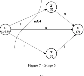
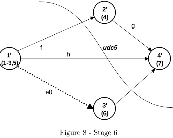
By the de…nitions we have adopted, arriving at a new stage means that an activity has been completed. The completed activity must be removed from the graph along with any nodes that are no longer linked to any un…nished activities. In some cases it will be necessary to substitute a dummy arc of zero duration for a completed activity (instead of removing the arc) because it is required that each activity be represented uniquely by its start and terminal node pair. (In other words, we do not allow for multigraphs where two or more arcs have identical start and terminal nodes.) Also the distribution of the remaining work-content (residual) must be determined for any activities that are in-progress (i.e., active) at the time a new stage begins. In general, determining the residual distribution for an arbitrary random variable is not a trivial task. This di¢ culty is avoided in this thesis by assuming that the work-contents of all the activities are exponentially distributed. Due to the ‘memoryless’property of the exponential, the distribution of the residual work-contents of the ongoing activities are identical to the original distributions. Once the aforementioned changes to the graph have been made, we re-sample the work content w of the residual graph and appeal again to the BB, setting the start time to tnow. (One may use the original
point we have a value of the project cost based on a single (random) realization of the project.
We now describe the ‘outer loop’.
The ultimate goal is to obtain the distribution of the total cost of the project, so the procedure to obtain a single point described in the ‘inner loop’is repeatedK times, each time securing a value for the optimal costv(k):
The ensemble of K values would give a fairly good idea about the distribution of the optimal project cost, on the basis of which management can make rational bidding/performance evaluation decisions.
Following this logic, if it is recognized that re-optimization whenever possible will only improve the outcome as compared to the static situation where re-optimization is disallowed, then the exact solution to the single stage (static) problem can be taken as an upper bound on the actual expected cost of the multi-stage (dynamic) problem. In cases where the project is very large it may be more practical to calculate bounds on the multi-stage result rather than use MCS to estimate the distribution. The next section discusses how a lower bound may be calculated on the actual expected cost for the multi-stage problem.
3.2
Calculation of Bounds
[$28;000;$30;000] then again there would be no need for formal estimation: the estimate of the project cost may be put at $29,000 since the maximal error committed by such an estimate shall not exceed1=28or 3:6%:In other cases a project may be so large that it may be simply impractical to use the multi-stage procedure outlined in the previous section to estimate the expected cost of the dynamic problem.
Another bene…t of good bounds is they serve as an error check to ensure that a given method is producing logically consistent results. Obviously if an optimiza-tion method produces an optimal soluoptimiza-tion that lies outside of mathematically proven bounds on the objective function, then it is evidence that either the optimization method is ‡awed or an error has been made calculating the bounds.
Fortunately the method applied here to determine a lower bound on the expected cost of the project (the SAN objective) is relatively simple. The basic idea comes from Jensen’s Inequality [18] which tells us that:
K(x; E[W]) EW[K(x; W)]
In words, the optimal cost of the (deterministic) project when the expected work content of each activity is used instead of the r.v. is not larger than the optimal expected cost of the project assuming the work content to be a r.v. for each activity. In our context, Jensen’s Inequality is a mathematical statement of the fact that uncertainty is always more expensive than certainty. Jensen’s Inequality is applicable in our case due to the convexity of the project cost function K(x; ): So putting
LB =K(x; E[W]):
gives us a lower bound on the expected cost for the multi-stage problem. In other words we can be assured that no matter what management strategy (the BB) we choose to employ for the multi-stage problem, the resulting expected project cost will always be larger than or equal to the lower bound given above.