Seismic Analysis and Reliability-based Design of Secondary Systems

ABSTRACT

SAIGAL, RAKESH KUMAR. SEISMIC ANALYSIS AND RELIABILITY-BASED DESIGN OF SECONDARY SYSTEMS. (Under the direction of Abhinav Gupta)

Seismic qualification of secondary systems such as piping is performed using the response spectrum method. Structural responses evaluated using response spectrum method are used for checking the design equations specified by the ASME Section III Boiler and Pressure Vessel (ASME BPV) Code. This dissertation addresses the topics of combining modal responses in response spectrum method and the reliability associated with the ASME design equations. In the method for combining modal responses, the validity of the existing

BIOGRAPHY

Rakesh Kumar Saigal received a Bachelor’s degree in Civil Engineering from Delhi College of Engineering, Delhi, India in May 1997. After that he worked in Larsen & Toubro ECC Construction Group, from July 1997 to April 1998, supervising construction for foundations and chimneys. Thereafter, he joined R.M. Software Solutions Pvt. Ltd., a company working in the field of risk assessment of structures. After working for 2 years in the company, he joined the Civil Engineering Department at North Carolina State University, Raleigh, NC as a doctoral student in August 2000. He is a student member of American Society of Civil Engineers (ASCE).

ACKNOWLEDGEMENTS

This research was supported by the Center for Nuclear Power Plant Structures Equipment and Piping at North Carolina State University. Resources for the center came from the dues paid by member organizations, US Department of Energy, National Science Foundation, Department of Civil, Construction and Environmental Engineering and College of Engineering at NC State University.

I would like to thank Prof. Abhinav Gupta for his constant guidance and inspiration

throughout the course of this research. I would also like to thank committee members: Prof. Ajaya Gupta, Prof Vernon Matzen and Prof. S.M. Rahman.

I would like to express special thanks to my parents Rajinder & Usha Saigal, for their

encouragement, support and love. Their wishes and blessings have been a constant source of inspiration in my studies at the university.

I would like to thank my brother Sanjiv and sister-in-law Archana for their love and support.

My deepest love and thanks to my wife, Deepti for her patience, dedication, love and support.

TABLE OF CONTENTS

Page

LIST OF TABLES... VII

LIST OF FIGURES ...VIII

PART I

INTRODUCTION...1

1. Introduction... 2

2. Rigid Response Coefficient ... 3

3. Reliability-Based Design of Piping Systems ... 5

4. Proposed Research... 6

5. Organization... 9

References... 11

PART II COMBINATION OF MODAL RESPONSES:

A CLOSED-FORM

FORMULATION FOR

RIGID RESPONSE COEFFICIENT...14

Abstract... 15

1. Introduction... 16

2. Rigid Response Coefficient for Floor Motion ... 20

3. Closed-Form Formulation: Frequency Domain Approach ... 23

4. Closed-Form Formulation: Time Domain Approach ... 25

5. Results... 28

6. Summary and Conclusions ... 31

PART III CLOSED-FORM FORMULATION FOR RIGID RESPONSE

COEFFICIENT : APPLICATION TO RESPONSE SPECTRUM

METHOD...43

Abstract... 44

1. Introduction... 45

2. Numerical Evaluation of αi and Closed-form Formulation... 48

3. Application to Response Spectrum Method for Floor Motion ... 51

4. Simplification of Iterative Procedure for Fourier Amplitudes... 54

5. Summary and Conclusions ... 58

References... 59

Appendix A... 71

PART IV RELIABILITY OF ASME DESIGN EQUATIONS FOR

DIFFERENT FAILURE MODES ...74

Abstract... 75

1. Introduction... 76

2. Reliability-Based Design ... 78

3. ASME Design Equations and Failure Criteria... 80

4. Performance Functions for Reliability Evaluations... 84

5. Implicit Reliability Levels: Code Calibration... 86

6. Summary and Conclusions ... 90

References... 91

Appendix A... 102

PART V SUMMARY,

CONCLUSIONS, AND RECOMMENDATIONS

FOR FUTURE RESEARCH... 116

LIST OF TABLES

Page

PART II COMBINATION OF MODAL RESPONSES: A CLOSED-FORM

FORMULATION FOR RIGID RESPONSE COEFFICIENT

1. Characteristics of Dominant Sinusoids in Floor Motion ... 34

PART III CLOSED-FORM FORMULATION FOR RIGID RESPONSE

COEFFICIENT: APPLICATION TO RESPONSE SPECTRUM

METHOD

1. Relative values of Fourier frequencies and amplitudes from time history of floor motion. ... 62 2. Relative values of Fourier frequencies and amplitudes from iterative

procedure of evaluating PSDF from floor response spectrum... 62 3. Relative values of Fourier frequencies and amplitudes from simplified

procedure of evaluating PSDF from response spectrum... 62

PART IV RELIABILITY OF ASME DESIGN EQUATIONS FOR

DIFFERENT FAILURE MODES

1. Types of distributions, mean values and coefficient of variations... 94 2. Coefficient of variations for Pressure and Moment for different service

levels ... 94 3. Diameter and thickness of pipes considered for evaluating reliability using

LIST OF FIGURES

Page

PART II

COMBINATION OF MODAL RESPONSES: A CLOSED-FORM

FORMULATION FOR RIGID RESPONSE COEFFICIENT

1. Rigid Response Coefficient for Pacoima Dam, (S16E, 1971) earthquake

record ... 35

2. Response Spectra for Pacoima Dam, (S16E, 1971) earthquake record.... 35

3. Properties of 3-story structure subjected to Pacoima Dam, (S16, 1971) earthquake record... 36

4. Floor Response Spectra for 3-Story Structure Subjected to Pacoima Dam, (S16E, 1971) earthquake record for 5 % Damping... 37

5. Rigid Response Coefficient for First Floor... 38

6. Rigid Response Coefficient for Second Floor ... 38

7. Rigid Response Coefficient for Third Floor ... 39

8. Ratio Ft for Different Durations of Pacoima Dam, (S16E, 1971) earthquake record... 39

9. Rigid Response Coefficient for Free-Field Ground Motion of Pacoima Dam (S16E, 1971) earthquake record... 40

10.Rigid Response Coefficient for Earthquake Motion at First Floor in 3-Story Structure ... 40

11.Rigid Response Coefficient for Earthquake Motion at Second Floor in 3-Story Structure ... 41

12.Rigid Response Coefficient for Earthquake Motion at Third Floor in 3-Story Structure ... 41

14.Variation of

(

)

PART III CLOSED-FORM FORMULATION OF RIGID RESPONSE

COEFFICIENT: APPLICATION TO RESPONSE SPECTRUM

METHOD

1. Properties of 3 story structure... 63 2. Comparison for Rigid Response Coefficient for Floor Motion of Pacoima

Dam, (S16E, 1971) earthquake record... 64 3. Comparison for Rigid Response Coefficient for Floor Motion of Pacoima

Dam, (S16E, 1971) earthquake record... 65 4. Floor Response Spectra for 3-Story Structure Subjected to Pacoima Dam,

(S16E, 1971) Earthquake record for 5 % damping... 66 5. Comparison of rigid response coefficient... 67 6. Comparison of rigid response coefficient... 68 7. Comparison of PSDF curves using iterative and simplified procedures .. 69 8. Comparison of rigid response coefficient... 70

PART IV RELIABILITY OF ASME DESIGN EQUATIONS FOR

DIFFERENT FAILURE MODES

1. Probabilistic Distribution for S, L and Z ... 96 2. Different conditions of stress distributions for plastic instability in pipe. 96 3. Load deformation curve for determination of collapse moment ... 97 4. Stress-Strain behavior for (a) elastic-perfectly plastic b) bilinear kinematic

6. Reliability index for elastic-perfectly plastic material and Service Level C... 99 7. Reliability index for elastic-perfectly plastic material and Service

Level D... 99 8. Reliability index for bilinear kinematic strain hardening material and

service Level C ... 100 9. Reliability index for bilinear kinematic strain hardening material and

PART I

1. Introduction

Seismic qualification of secondary systems such as piping in nuclear power plants is based on the response spectrum method of analysis. Accuracy of response quantities evaluated using response spectrum method is highly dependent upon the process of combining modal responses. The resultant moments in various pipe components evaluated from such an analysis are then used for evaluating the safety of the design by using the design equations specified by the ASME Boiler, Pressure Vessel and Piping Code, Section III (ASME 2004). This dissertation is aimed at studying two aspects within this process, one that relates to the process of combining modal responses in the response spectrum method, and the other that relates to the ASME Section III design equations. Both these aspects have gained significant attention within the profession in recent years (USNRC 1999, Hahn and Valenti 1997, Ayyub et. al.1995, ASME 2002). Recent research projects in both these areas (USNRC 1999,

ASME 2002) have identified specific limitations in the existing state-of-the-art and have emphasized the need for additional studies to overcome them. With respect to the methods for combining modal responses, this dissertation focuses on evaluating the validity of

consistency in reliability of structural components has been achieved by formally addressing uncertainty and randomness using probabilistic analysis (Galambos et. al. 1982, Rackwitz and Feissler 1978, Ellingwood 1982). While some exploratory studies have been conducted on evaluating the Load and Strength Factors for piping systems, significant work is needed for conducting calibration studies of the existing code equations before target reliabilities for developing load and strength factors are justified. In this dissertation, a calibration study is conducted for performance functions that characterize the design limit-states for various load cases. The following sections provide somewhat detailed discussion on the background of existing work in both these areas.

2. Rigid Response Coefficient

Structural responses evaluated in the response spectrum method of seismic analysis and design are highly dependent upon the process of combining modal responses. Most of the studies conducted on this subject have focused on evaluating the modal correlation coefficient which gives the correlation between modes with closely spaced frequencies (Rosenblueth and Elorduy 1969, Singh and Chu 1976, Der Kiureghian 1980, Gupta 1992, Gupta et. al. 1997, Hahn and Valenti 1997). Modes with closely spaced frequencies are combined according to the following double-sum equation

∑∑

∑

≠ + =

i j i

j i ij i

i RR

R

R2 2 ε

proposed, the Complete Quadratic Combination (CQC) represents one widely popular definition for εij. A key limitation of the double-sum equation is that it cannot account for

correlation between two modes whose frequencies are sufficiently apart and also greater than the rigid frequency of earthquake motion. In such a case, the above equation results in

Square-Root-Sum-of-the-Squares (SRSS) combination because εij→ 0. The response in two

high frequency modes should truly be combined algebraically because the high frequency modes are perfectly correlated with the ground motion and consequently perfectly correlated with each other.

Recently, USNRC (1999) conducted a research study to evaluate various methods of combining modal responses. This study recommends the use of rigid response coefficient in conjunction with modal correlation coefficient. It should be noted that the modal response does not change abruptly from damped periodic to rigid beyond the rigid frequency. Gupta (1992) used free-field earthquake records to numerically evaluate the variation of rigid response coefficient between the low frequency region to the high frequency region. This variation is then represented as linear on a semi-log plot. In addition to the extensive research on rigid response coefficient presented in Gupta (1992), Lindley-Yow’s (1980) method appears to be most rational for modes with frequencies in the vicinity of rigid frequency. However, its primary criticism has been related to its heuristic basis for defining the rigid response coefficient which gives highly incorrect results for low frequency modes (USNRC 1999). More recently Hahn and Valenti (1997) used a frequency domain approach to evaluate an expression for modal correlation coefficient εij. Unlike CQC, which is based on the

implicitly considers the “rigid” and “damped-periodic” parts. In the limit, the expression for εij proposed in their work can be shown to converge towards that for the rigid response

coefficient. The variation of rigid response coefficient evaluated by this expression is linear between low and high frequency region and similar in nature to that proposed by Gupta (1992) and Gupta et al. (1997). All the existing formulations have been developed and evaluated for the case of free-field ground motions. Unlike buildings, the earthquake input at the base of secondary systems such as piping is characterized in terms of floor response spectrum which represents a motion filtered through the building. Applicability of existing rigid response coefficient formulations to the case of floor motion is not explicitly evident because the frequency characteristics of a filtered floor motion are very different from those of a free-field ground motion.

3. Reliability-Based Design of Piping Systems

The current design codes such as Section III of American Society of Mechanical Engineers (ASME) Boiler and Pressure and ASME B31 codes (2004) rely on the traditional Working Stress Design (WSD) format in which safety factors are prescribed deterministically. These deterministic safety factors are based on observations and experience from the test data. Designs based on WSD methodology can lead to excessive conservative designs that can have widely varying reliability of piping components. In recent years, consistency in

nominal values of strength and loads, respectively, which are considered as random

variables. The γi and φ are partial safety factors for load and strength and are determined for a

particular (target) reliability. A reliability-based design provides risk consistency and is likely to result in more economical use of materials, design compatibility for different materials, and permits future modifications due to increase knowledge of failure mechanisms, material characterization, and loading environment.

Probabilistic methodologies such as LRFD have been incorporated in the design codes by several organizations such as American Institute of Steel Construction (AISC) and the American Concrete Institute (ACI). LRFD methodology for ship structures was proposed by Ayyub et. al. (1995) and Assakkaf et. al. (2000), and for reinforced concrete structures by Mirza (1996). An exploratory study on LRFD based piping design was presented by Gupta and Choi (2003). The design rules as specified in the ASME Section III vary according to the failure criteria. In order to develop LRFD based design rules for the ASME piping codes, it is essential to evaluate the reliability levels associated with the existing design equations. This process, called as code calibration, helps in establishing target reliability levels for LRFD based design rules. In this dissertation, we present one such exploratory study that evaluates reliability levels associated with the existing design equations for straight pipe segments.

4. Proposed Research

4.1 Rigid Response Coefficient

This research is divided into two parts – (a) Develop a closed-form formulation for rigid response coefficient, and (b) Further simplification of the closed-form formulation for application to the response spectrum method. The specific sub-tasks needed are: • Evaluate the applicability of existing rigid response coefficient formulations to the

case of floor motions.

a) Generate floor motion for sample structural system.

b) Use the floor motion to evaluate the rigid response coefficient numerically. c) Compare with the values obtained using existing formulations.

• Develop a closed-form formulation for rigid response coefficient using time domain approach.

• Simplify the closed-form formulation to eliminate the effect of earthquake duration. • Compare the results with the numerically evaluated results for ground motion. • Compare the results with the numerically evaluated results for floor motion.

• Use the closed-form expression to explain the nature of variation for rigid response coefficient in case of floor motion.

4.2 Reliability-Based Design of Piping Systems

• Characterize the random variables and their statistical properties that define the loads and strength.

• Define the performance function for class 2 piping in accordance with the Equation 9 of NC 3600, ASME Section III for service levels given below

m e

S Z

M B t PD

B 1.5

2 2

1 + ≤ for Level A

m e

S Z

M B t PD

B 1.8

2 2

1 + ≤ for Level B

m e

S Z

M B t PD

B 2.25

2 2

1 + ≤ for Level C

m e

S Z M B t PD

B 3

2 2

1 + ≤ for Level D

where,

BB1 and B2B are primary stress indices for the specific piping component

P is the design pressure

D is the average diameter of the pipe

t is the thickness of the pipe

Ze elastic section modulus of the pipe

M is the resultant moment due to combination of different loads

• Characterize the performance function for the different failure criteria given below a) Onset of yielding in the pipe

b) Formation of single plastic hinge

c) Plastic Instability as defined by stress in outermost fiber reaching ultimate strength Su, based on a linear elastic analysis.

d) Plastic Instability as defined by the occurrence of collapse moment corresponding to twice-the-elastic slope in a moment-curvature curve as defined in ASME code.

• Develop closed-form expression for moment- curvature relationship.

• Calibration of reliability of existing equations with respect to various failure criteria.

5. Organization

This dissertation consists primarily of three manuscripts which will be submitted for possible publications in peer reviewed journals. The first manuscript, Part II of the dissertation, evaluates the applicability of the existing rigid response coefficient formulations for the case of floor motion. A closed-form formulation is developed and its accuracy is evaluated by comparison with rigid response coefficient values evaluated numerically using time history analysis for both the ground and the floor motions. The second manuscript in this

The third manuscript in this dissertation, Part IV, is an exploratory study on the reliability-based design of piping systems. An attempt is made to evaluate the minimum reliability associated with performance functions corresponding to ASME design equations for a straight pipe. The reliability is evaluated by formulating a moment-curvature

relationship for a straight pipe based on elastic-plastic and bilinear kinematic hardening material models.

References

ASME (2002), “Development of alternative reliability-based load and resistance factor design methods for piping”, A proposal submitted to ASME Center for Research and Technology Development, developed by the ASME working group on piping design, endorsed by ASME code committee and ASME research committee on risk technology. ASME (2004), Rules for construction of nuclear facility components, ASME Boiler and

Pressure Vessel Code, Section III, American Society of Mechanical Engineers. Assakkaf, I.A., Ayyub. B.M., and Mattei, N. J. (2000), “Reliability-Based Load and

Resistance Factor Design (LRFD) of Hull Structural Components of Surface Ships.”

Association of Scientists and Engineers, 37th Annual Technical Symposium, ASE. Ayyub, B.M., Beach J. and Packard, T. (1995), “Methodology for the development of

reliability-based design criteria for surface ship structures”, Naval Engineers Journal, ASNE, 107(1), 45-61.

Der Kiureghian, A. (1980), “A response spectrum method for random vibrations”, Report No. UCB/EERC-80//15, Earthquake Engineering Research Center, University of California, Berkeley, California.

Ellingwood, B. (1982) “Probability based load criteria-load factors and load combinations” ,

Journal of Structural Division, ASCE, 108(5), 978-997.

Gupta, A.K. (1992), Response Spectrum Method in Seismic Analysis and Design of Structures, CRC Press, Boca Rotan, Florida.

Gupta, A. and Choi, B.(2003), “Reliability-based load and resistance factor design for piping: An exploratory case study”, Nuclear Engineering and Design, v 224, n 2, 161-178. Gupta A.K., Hassan T and Gupta A. (1997), “Correlation coefficients for modal response

combination of non-classically damped systems”, Nuclear Engineering and Design,165(1-2), 67-80.

Hahn, G.D. and Valenti, M.C. (1997), “Correlation of seismic responses of structures”,

Journal of Structural Engineering, 123(4), 405-413.

Lindley, D.W. and Yow, J.R. (1980), “Modal response summation for seismic qualification”,

Second ASCE Specialty Conference on Civil Engineering and Nuclear Power, VI, Paper 8-2, Knoxville, TN.

Mirza, S.A. (1996), “Reliability based design of reinforced concrete columns”, Structural Safety, 18, 179-194.

Rackwitz, R. and Fiessler, B. (1978), “Structural stability under combined random load sequences”, Computers and Structures, 9, 489-584.

Rosenblueth, E. and Elorduy, J. (1969), “Response of linear system in certain transient disturbances”, Proceedings, Fourth World Conference in Earthquake Engineering ,

Santiago, Chile, A-1, 185-196.

Part II

COMBINATION OF MODAL RESPONSES:

A CLOSED-FORM FORMULATION FOR

RIGID RESPONSE COEFFICIENT

Rakesh K. Saigal and Abhinav Gupta

Combination of Modal Responses: A Closed-Form Formulation for Rigid

Response Coefficient

Rakesh K. Saigal and Abhinav Gupta

Abstract

Recent studies conducted by US Nuclear Regulatory Commission (USNRC) for combining modal responses in a response spectrum method of seismic analysis and design have

emphasized that each modal response quantity should be separated into damped-periodic and rigid parts before combining the contributions from different modes. The damped periodic parts of modal responses are combined using the double-sum equation whereas the rigid parts are combined algebraically. A particular modal response quantity is separated into damped-periodic and rigid parts using the “rigid response coefficient”. The USNRC sponsored study recommends the calculation of rigid response coefficient by either the Lindley-Yow

of a floor motion are very different from those of a free-field ground motion. In this paper, we study the validity of existing formulations for the case of floor motions and develop a closed-form solution based on a time domain approach to explain the behavior of rigid response coefficient. The formulation is then used to explain the nature of variation in rigid response coefficient for ground and floor motions. It is shown that the proposed formulation and its simplified form gives results that are identical to those evaluated numerically in the complete frequency region of interest.

1. Introduction

Structural responses evaluated in the response spectrum method of seismic analysis and design are highly dependent on the process of combining modal responses. Most of the studies conducted on this subject have focused on evaluating the modal correlation coefficient which gives the correlation between modes with closely spaced frequencies (Rosenblueth and Elorduy 1969, Singh and Chu 1976, Der Kiureghian 1980, Gupta 1992, Gupta et. al. 1997, Hahn and Valenti 1997). Modes with closely spaced frequencies are combined according to the following double-sum equation

(1)

∑∑

∑

≠ + =

i j i

j i ij i

i RR

R

R2 2 ε

in which Ri and Rj are responses in modes i and j, respectively; and εij is the correlation

coefficient between modes i and j. Among the several definitions of εij that have been

for εij. A key limitation of the double-sum equation is that it cannot account for correlation

between two modes whose frequencies are sufficiently apart and also greater than the rigid frequency of earthquake motion. In such a case, the above equation results in Square-Root-Sum-of-the-Squares (SRSS) combination because εij→ 0. The response in two high

frequency modes should truly be combined algebraically because the high frequency modes are perfectly correlated with the ground motion and consequently perfectly correlated with each other.

A few studies have presented rules for combining responses in the high frequency modes (Lindley and Yow 1980, Kennedy 1979, Hadjian 1981, Singh and Mehta 1983, Gupta 1992, Der Kiureghian and Nakamura 1993, Gupta et al. 1997). These studies have proposed an additional correlation coefficient which is referred to as “rigid response coefficient”. The concept of rigid response coefficient αi is related to the observation that, as the ith modal

frequency increases, a greater fraction of the modal response is correlated with the

earthquake motion at the structure’s base. It must be noted that the response in a mode with frequency greater than the rigid frequency of earthquake input at the structure’s base is completely correlated with the base motion. Recently, the USNRC (1999) conducted a research study to evaluate various methods of combining modal responses. This study recommends the use of rigid response coefficient in conjunction with modal correlation coefficient. Existing studies classify the response in low frequency modes as “damped-periodic” p and the response in high frequency modes as “rigid” , where R

i

R r

i

R i is the

i i r

i R

R =α p _{i i}

i R

R _{= 1−α}2 ₍₂₎

For any two modes, the damped periodic responses are combined correctly by the double-sum method and the rigid responses are combined algebraically:

( )

_∑

( )

_∑∑

≠ + =

i j i

p j p i ij i

p i

p _{R R R}

R 2 2 2 ε r

i

r _R

R =

∑

The damped-periodic and the rigid parts are then combined as follows:

( ) ( )

2 _Rp _Rr

R = + . (4)

The above equations can be combined to rewrite Eq.(1) as a modified double-sum equation:

∑∑

∑

≠ + =

i j i

j i ij i

i R R

R

R2 2 2 ε _,

(

)(

)

ij j i

ij α α ε α α

ε = + − − (5)

It should be noted that the modal response does not change abruptly from damped periodic to rigid beyond the rigid frequency. Gupta (1992) used free-field earthquake records to numerically evaluate the variation of rigid response coefficient between the low frequency region to the high frequency region. This variation is then represented linearly on a semi-log plot. In addition to the extensive research on rigid response coefficient presented in Gupta (1992), Lindley-Yow’s (1980) method appears to be most rational for modes with

recently, Hahn and Valenti (1997) used a frequency domain approach to evaluate an expression for modal correlation coefficient εij. Unlike CQC, which is based on the

assumption of white noise excitation, Hahn and Valenti (1997) consider excitations with narrow, intermediate, and wide frequency bandwidths. This formulation implicitly considers the “rigid” and “damped-periodic” parts. In the limit, the expression for εij proposed in their

work converges to that for the rigid response coefficient. The variation of rigid response coefficient evaluated by this expression is linear between low and high frequency region and similar in nature to that proposed by Gupta (1992) and Gupta et al. (1997).

2. Rigid Response Coefficient for Floor Motion

Numerically, the correlation between earthquake input acceleration at the base and the total acceleration response of a Single Degree of Freedom Oscillator (SDOF) having a

b

u

t i

u

frequency fi can be evaluated as:

∫

∫

∫

where Td is the duration of the input earthquake motion. The above definition is based on the

assumption that is a stationary ergodic process (Newland 1993). USNRC (1999) recommends the following definition of α

b

u

i which is based on the work of Gupta (1992).

According to this definition, αi for a SDOF oscillator is defined linearly between two key

frequencies f 1 and f 2on a semi-logarithmic plot and is given by

(

)

(

)

1 / ln / ln f f f f_i i= α , max max 1 2 _V A S S f π

= , _f 2_{= f}r (7)

where, SAmax and SVmax are maximum values of pseudo spectral acceleration and velocity,

respectively. The frequency f r represents the rigid frequency of input motion i.e. the

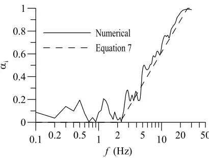
frequency beyond which the acceleration response is independent of damping. Fig. 1 shows the variations of αi with oscillator frequencies fi evaluated numerically using Eq.(6) and

evaluated using Eq.(7) for the Pacoima Dam, (S16E, 1971) earthquake record. The

gives a definition of αi that works well for the case of free field ground motion record. To

understand the definitions of the key frequencies f 1 and f 2 , let us examine the spectral shapes for the input motion. The key frequency f 1 corresponds to the dominant frequency of the input motion and the value of αi below f 1 is taken as zero. The correlation between rigid

parts increases with increasing oscillator frequency such that αi = 1 at fi = f 2 where spectra

becomes independent of damping.

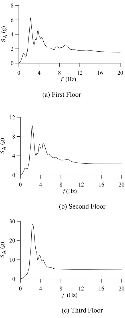
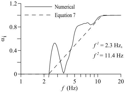
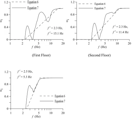
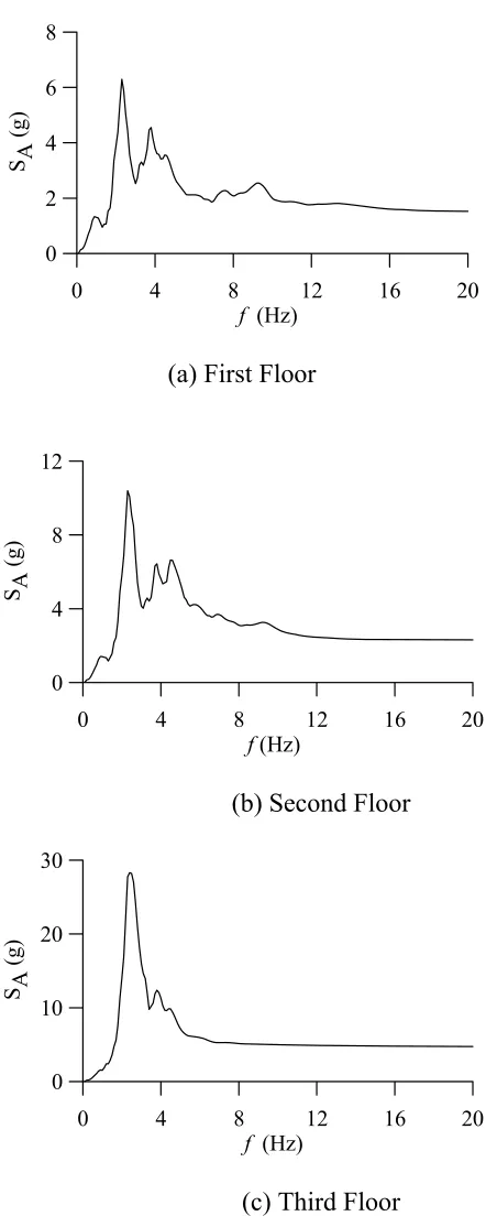
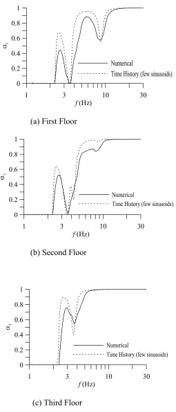
Next, we examine the validity of Eq.(7) for the case of filtered earthquake motion, i.e. floor motion which represents earthquake input at the base of secondary systems. To do so, we consider a 3-story shear building, shown in Fig. 3, that is subjected to Pacoima Dam, (S16E, 1971) earthquake record at its base. The acceleration time histories for floor motion at each of the three floors are obtained from a direct integration of the equations of motion for the 3-story structure which is considered to have 5% damping in all the three modes. The floor response spectrum at each floor is shown in Fig. 4. The floor spectra are characterized by well defined narrow banded peaks that occur in the vicinity of modal frequencies for the 3-story structure. We evaluate the rigid response coefficients for each of the three floor motions numerically using the respective acceleration time histories as well as using the definition given by Eq.(7). The two sets of curves are compared in Figs. 5-7. The key frequencies f 1and f 2 needed for evaluating αi values in Eq.(7) at each floor are specified in

the figures. These figures provide a valuable observation that the straight line variation of αi

In the case of a floor motion, the earthquake record consists primarily of a few sinusoids each of which can have a relatively large amplitude, as is evident from the existence of multiple narrow banded peaks in the response spectra. Some of these peaks occur at frequencies which are much higher than the low frequency region corresponding to the amplified region in the free-field ground response spectra. The response of an oscillator in the vicinity of a spectral peak is dominated by the damped-periodic part resulting in a relatively lower value of αi in that region. The response of an oscillator becomes increasingly

rigid as its frequency becomes further apart from the dominant frequencies of input motion. This behavior is clearly evident in Figs. 5 and 6 in which αi approaches zero in the vicinity of

2.4 Hz and 4.0 Hz, the first two frequencies of the 3-story building. In the vicinity of 8.8 Hz, the αi values becomes relatively low but not zero because the amplitude of the input pulse

associated with the third structural mode is not significant as can be seen from the relative values of the spectral acceleration at these frequencies in Fig. 2. Unlike floor motion, the dominant frequencies in a free-field earthquake motion occur in the low-frequency region as seen in Fig. 2. The free-field motion consists of several sinusoids with frequencies in mid to high frequency region, resulting in relatively broad-banded spectral curve. Therefore, the rigid response coefficient exhibits a gradual increase in its value. The mid to high frequency input pulses simply result in localized peaks and valleys of numerically calculated αi values

between f 1_{and f} 2 _{as seen in Fig. 1. Consequently, Eq.(7) works well for free-field motion}

by representing the overall behavior of αi. Next, we develop a closed-form formulation that

3. Closed-Form Formulation: Frequency Domain Approach

A closed-form solution for rigid response coefficient can be developed using either a time or a frequency domain approach. In frequency domain approach, Eq.(6) can be rewritten in the following form (Price and Bishop 1974)

( )

( )

_∫

( )

∫

∫

where ω is the frequency in rad/s; Srr represents the power spectral density function (PSDF)

for the response of an SDOF system; t S

i

u bb is the PSDF of the earthquake input motion at

the base of the SDOF system; and S

b

u

rb(ω) is the cross power spectral density function between

and , respectively. The power spectral density functions are defined as

t i

u u_b

( )

( ) ( )

rb H S

S = S_rr

( )

( )

( )

in which Hr(ω) is the complex-valued frequency response function for the response . For

an oscillator with frequency ω

t i

u

i and damping ratio ζiwe can write

( )

Closed-form evaluation of integrations in Eq.(8) is quite formidable for excitations that are not white noise. Hahn and Valenti (1997) attempted such a closed-form evaluation for narrow, intermediate, and broad-banded excitation by rewriting Eq.(9) in the following form

H_r

( )

( )

[

(

( )

)

]

where,

( )

( )

( )

( )

( )

( )

( )

( )

1 2 1

i i

i , _ω

ω ω ν ω ω ζ ω ν = = −

However, Hahn and Valenti(1997) substituted simple approximate functions for ν1(ω) and ν2(ω) to facilitate the integration of Eq.(8) . They chose

ν₁

( )

( )

ν₂ 2 1 (12)

The final expression evaluated by such an approximation can be written in the following form

( )

= (13)

in which f 1 and f 2 are two key frequencies similar in nature and definition to those given by Gupta(1992). Eq.(13) results in a variation of αi that is very similar in nature to that given by

Eq.(7). The key difference lies in the consideration of modal damping ζi in the evaluation of αi by Eq.(13). The effect of damping is similar to that given by Gupta et al. (1997) in another

numerical study.

4. Closed-Form Formulation: Time Domain Approach

To avoid the assumptions of Eq.(12) described above, we develop a closed-form solution in the time domain. If the earthquake input time history at a structure’s base can be represented by a Fourier series, a formulation for αi can be developed by using the steady-state response

of a SDOF oscillator and the Fourier series of base motion in Eq.(6). The Fourier series for n

sinusoids in the base input motion can be written as

(

∑

=

+ = n

j

j j bj

b u t

u

1

sin Ω φ

)

)

(14)

where is the absolute base acceleration at time t, is the maximum base acceleration, Ω

b

u u_bj

j is the excitation frequency, andφj is the phase angle of the jth pulse. The steady-state

response of an SDOF oscillator having natural frequency ωi and damping ratio ζi , subjected

to the harmonic input defined by Eq.(14) can be written as

(

∑

=

− + = n

j

ij j j bj

ij t

i u t

u

1

sinΩ φ ψ

where,

(

)

(

) (

)

2 2 1 2 1 ij i ij ij i ij β ζ β β ζ λ + − +

= , βij = Ωj / ωi , _⎟⎟

⎠ ⎞ ⎜ ⎜ ⎝ ⎛ + − = − 2 2 3 1 ) 2 ( ) 1 ( 2 ij ij ij i

ij Tan _{β ζβ}

β ζ

ψ (16)

A closed-form integration of Eq.(6) after substituting Eqs.(14) and (15) can be expressed as

(

)

(

)

(

)

(

)

(

)

( )

(

)

( )

(

)

( )

∑∑

∑

∑∑

Eq.(17) is exact and has been derived without any simplifications or approximations. To simplify the above equation, it is rewritten as

t

i F

CE A

=

α (18)

where,

(

)

(

) (

)

X

F_t = = =

+ + + = , , , 1 1 1

It must be noted that the quantities A, C and E contain terms with duration Td whereas the

quantities B, D and F are purely sinusoidal. For typical values of earthquake duration (Td =

43.8 seconds for Pacoima Dam, S16E, 1971 earthquake record), the ratio Ft is close to unity

as shown in Fig. 8. Therefore, Eq.(18) can be further simplified as

E C

A

i =

The quantities A, C, and E are also dominated by the relatively large values of Td and can be

further simplified for the same reasons as explained above.

( )

_∑

_∑

∑

Such simplification also allows for Td to be factored out of the equation. Therefore, a

simplified form for the rigid response coefficient can be written as

(

)

∑

∑

∑

α (21)

It can be seen that the final expression does not contain any term with phase (φ) of the ground motion.

5. Results

The closed-form equation for rigid response coefficient is now applied to an SDOF system subjected to free-field Pacoima Dam, (S16E, 1971) earthquake record. The Fourier series for the earthquake record is developed using 216 sample points between 0 to 30 Hz. The

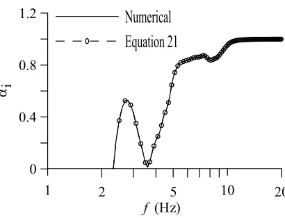
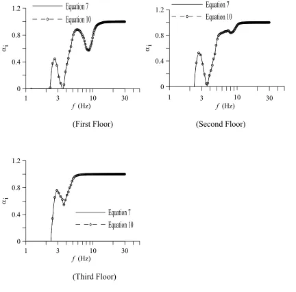
Fig. 3. The rigid response coefficient for each floor is then compared to the numerically evaluated values from Eq.(6). The results are compared in Figs. 10-12 which show that Eq.(21) and numerically evaluated results are almost identical.

The closed-form formulation of Eq.(21) can be used to further explain the observed variation of αi for the case of floor motions. As mentioned earlier, a Fourier series

corresponding to the floor motion consists of only a few dominant sinusoids whose frequencies lie in the vicinity of structural frequencies. For the 3-story shear building

considered in this study, the Fourier amplitudes, the frequencies, and the phase angles for the three predominant sinusoids in the vicinity of structural frequencies are given in Table 1. Let us begin with the motion at first floor for which the sinusoids at 2.3 Hz and 3.7 Hz have relatively larger amplitudes.

• In the vicinity of 2.3 Hz, the response of an oscillator is not in phase with the ground motion as βi≈ 1 and the phase angle ψi≈ π/2 radians. Consequently the αi values in

this region are close to zero. Also note that the key frequency f 1 corresponds to the frequency of the most dominant pulse.

• As the oscillator frequency increases beyond 2.3 Hz, the frequency ratio βi < 1 and

the phase angle ψiapproaches zero. When fi > f r, βi≈ 0 , ψi≈ 0 indicating that the

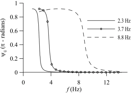
modal maximas always occur at the same time and combine algebraically. • As shown in Fig. 13, for 0 ≤βi≤ 1, the phase ψilies between 0 and π radians,

indicating that a certain fraction of modal maximas always combine algebraically. This fraction is represented by the rigid response coefficient.

• For an oscillator frequency between 2.3 Hz and 3.7 Hz, βi < 1 with respect to 2.3 Hz

in value as the oscillator frequency increases beyond 2.3 Hz because βi with respect

to 2.3 Hz is significantly less than unity but βj with respect to 3.7 Hz approaches

unity.

• It should be noted that for fi = 3.7 Hz, the amplitude of the steady-state response λij übj≈ 1 with respect to 2.3 Hz input pulse and is relatively smaller than the

amplitude of response λij übj≈ 8 with respect to 3.7 Hz input pulse as seen in Fig. 14.

Therefore, the steady-state response due to 3.7 Hz input pulse dominates the total response but it is not in-phase with the ground motion as ψi≈ π /2. Consequently, we

notice that αi approaches zero in this frequency region.

• Beyond 3.7 Hz, αi once again starts increasing in value. Its value decreases once

again in the vicinity of 8.9 Hz, the frequency corresponding to the third input pulse in Table 1. However, this decrease is small because the amplitude of steady-state

response due to 8.9 Hz input pulse does not dominate the total response. Instead, the responses due to 2.3 Hz and 3.7 Hz input pulse are relatively significant when

fi≈ 8.9 Hz.

• A similar behavior can be seen in the variation of αi values corresponding to the

second floor.

• For the third floor, it can be observed in Table 1 that the Fourier amplitude corresponding to the 8.8 Hz frequency pulse is relatively small, as is also evident from the rigid response coefficient for this floor in Fig. 12. Thus, the αi values do not

6. Summary and Conclusions

This paper presents a discussion on the “rigid response coefficient” needed in the response spectrum method for combining modal response quantities. It is shown that the existing definitions for the rigid response coefficient are a good representation of the overall behavior in case of a free-field motion. However, it is also observed that the definition does not work well in case of floor motions which are used as input in the seismic analysis of secondary systems such as piping and equipment. A closed-form formulation is developed to

References

Der Kiureghian, A. (1980), “A response spectrum method for random vibrations”, Report No.UCB/EERC-80//15, Earthquake Engineering Research Center, University of California, Berkeley, California.

Der Kiureghian, A. D. and Nakamura, Y. (1993), “CQC modal combination rule for high frequency modes”, Earthquake Engineering and Structural Dynamics, 22, 943-956. Gupta, A.K. (1992), Response Spectrum Method in Seismic Analysis and Design of

Structures, CRC Press, Boca Rotan, Florida.

Gupta A.K., Hassan T and Gupta A. (1997), “Correlation coefficients for modal response combination of non-classically damped systems”, Nuclear Engineering and

Design,165(1-2), 67-80

Hadjian, A.H. (1981), “Seismic response of structures by response spectrum method”,

Nuclear Engineering and Design, 66(2), 179-201.

Hahn, G.D. and Valenti, M.C. (1997), “Correlation of seismic responses of structures”,

Journal of Structural Engineering, 123(4), 405-413.

Kennedy, R.P. (1979), “Recommendations for changes and additions to standard review plans and regulatory guides dealing with seismic design requirements for structures”,

NUREG/CR-1161, Report prepared for Lawrence Livermore Laboratory.

Lindley, D.W. and Yow, J.R. (1980), “Modal response summation for seismic qualification”,

Newland, D.E. (1993), An introduction to random vibrations, spectral and wavelet analysis, 3rd edition, Prentice Hall

Price, W.G. and Bishop, R.E.D. (1974), Probability theory of ship dynamics, Chapman and Hall Ltd., London, England.

Rosenblueth, E. and Elorduy, J. (1969), “Response of linear system in certain transient disturbances”, Proceedings, Fourth World Conference in Earthquake Engineering,

Santiago, Chile, A-1, 185-196.

Singh, M.P. and Chu, S.L. (1976), “Stochastic considerations in seismic analysis of structures”, Earthquake Engineering and Structural Dynamics, 4, 295-307.

Singh, M.P. and Mehta, K.B. (1983), “Seismic design response by an alternative SRSS rule”,

Earthquake Engineering and Structural Dynamics, 11, 771-783.

USNRC (1999), Reevaluation of Regulatory Guidance on Modal Response Combination Methods for Seismic Response Spectrum Analysis, Brookhaven National Laboratory, U.S. Nuclear Regulatory Commission Office of Nuclear Regulatory Research,

Table 1: Characteristics of Dominant Sinusoids in Floor Motion

Ωi(Hz) Normalized übj φi (radians)

DOF i = 1 i = 2 i = 3 i = 1 i = 2 i =3 i = 1 i = 2 i = 3

0.1 0.2 0.5 1 2 5 10 20 50

f (Hz)

0 0.2 0.4 0.6 0.8 1

αi

Numerical Equation 7

Fig. 1: Rigid Response Coefficient for Pacoima Dam, (S16E, 1971) earthquake record

0 10 20

f (Hz) 30

0 1 2 3 4 5

SA

(g

)

2% damping 5% damping

k1= 140000 kN/m

m1 = 122950 kg

k2= 140000 kN/m

m2 = 122950 kg

k3= 17500 kN/m

m3 = 52700 kg

Natural frequencies

f1 = 2.4 Hz

f2 = 4.0 Hz

f3 = 8.8 Hz

u1

u2

u3

k1

m1

m2 3

k3

k2

m

0 4 8 12 16 20

f (Hz) 0

2 4 6 8

SA

(g

)

(a) First Floor

0 4 8 12 16 20

f(Hz) 0

4 8 12

SA

(g)

(b) Second Floor

0 4 8 12 16 20

f (Hz) 0

10 20 30

SA

(g

)

(c) Third Floor

1 2 5 10 20

f (Hz) 0

0.4 0.8 1.2

αi

Numerical

Equation 7

f 1 = 2.3 Hz,

f 2_{= 15.1 Hz}

Fig. 5: Rigid Response Coefficient for First Floor

1 2 5 1

f (Hz) 0 20

0 0.4 0.8 1.2

αi

Numerical Equation 7

f 1 _{= 2.3 Hz,}

f 2= 11.4 Hz

1 2 5 10 20

f (Hz) 0

0.4 0.8 1.2

αi

Numerical Equation 7

f 1 _{= 2.5 Hz,}

f 2_{= 5.3 Hz}

Fig. 7: Rigid Response Coefficient for Third Floor

0 5 10 15 20 25 30

f (Hz) 0

0.5 1 1.5 2

Ft

Td = 43.8 s

Td = 50 s

Td = 60 s

1 2 5 10 20 50 0.5

f (Hz)

0 0.4 0.8 1.2

αi

Numerical Equation 21

Fig. 9: Rigid Response Coefficient for Free-Field Ground Motion of Pacoima Dam (S16E, 1971) earthquake record

1 2 5 10 20

f (Hz) 0

0.4 0.8 1.2

αi

Numerical Equation 21

1 2 5 10 20

f (Hz) 0

0.4 0.8 1.2

αi

Numerical Equation 21

Fig. 11: Rigid Response Coefficient for Earthquake Motion at Second Floor in 3-Story Structure

1 2 5 1

f (Hz) 0 20

0 0.4 0.8 1.2

αi

Numerical Equation 21

0 4 8 12

f(Hz) 0

0.2 0.4 0.6 0.8 1

ψij

(

π

- rad

ians)

2.3 Hz 3.7 Hz 8.8 Hz

Fig. 13: Variation of ψi between f 1 and f 2 for First Floor

0 4 8 12

f(Hz) 0

4 8 12

λij

*übj

2.3 Hz 3.7 Hz 8.8 Hz

Part III

CLOSED-FORM FORMULATION FOR RIGID RESPONSE

COEFFICIENT: APPLICATION TO RESPONSE SPECTRUM

METHOD

Abhinav Gupta and Rakesh K. Saigal

Closed-Form Formulation for Rigid Response Coefficient: Application to

Response Spectrum Method

Abhinav Gupta and Rakesh K. Saigal

Abstract

In the response spectrum method of seismic analysis and design, the design response is evaluated by combining contributions from individual modal responses. For this purpose, each individual modal response quantity is separated into two parts, the damped-periodic part and the rigid part. The damped-periodic parts are combined using the double-sum method which accounts for the correlation between modes with closely-spaced frequencies. The rigid parts are completely correlated with each other and combined algebraically. Separation of the individual modal response quantities into the damped-periodic and the rigid parts is

accomplished by using another correlation coefficient referred to by “rigid response

coefficient.” Recently, the US Nuclear Regulatory Commission revised the Regulatory Guide 1.92 and recommended that the rigid response coefficient be evaluated by using the

definitions proposed by either Lindley-Yow (1980) or Gupta (1992). Lindley-Yow’s

response coefficient do not work well for the case of floor motions. A closed-form formulation is developed to explain the concept of rigid response coefficient. This closed-form closed-formulation requires knowledge of Fourier amplitudes and gives rigid response coefficient values that are identical to the numerically calculated values for both the ground motion and floor motion. However, it cannot be extended directly to the response spectrum method. Consequently, we formulate a simplified method to evaluate the relative values of Fourier amplitudes from the floor response spectrum. The method together with the closed-form closed-formulation gives results which are relative less accurate but acceptable within the domain of response spectrum method

1. Introduction

In seismic analysis and design, structural response evaluated using response spectrum method is dependent on the process of combining contributions from individual modes. Conventionally, the responses are combined according to the double-sum equation

∑∑

∑

= + =

i j i

j i ij i

i RR

R

R2 2 ε ₍₁₎

where, Ri and Rj are responses in modes i and j, respectively; and εij is the modal correlation

coefficient between modes i and j. Several different researchers have developed expressions for εij to account for correlation between modes with closely-spaced frequencies (Der

closely-spaced frequencies. Gupta (1992) modified the double-sum equation in which εij is

replaced by a new correlation coefficient ε_ijto account for correlation between high frequency modes, i.e.,

∑∑

∑

≠ + =

i j i

j i ij i

i R R

R

R2 2 2 ε _,

(

)(

)

ij j i

ij α α ε α α

ε = + − − (2)

in which αi and αj are the rigid response coefficient in modes i and j, respectively. USNRC

Regulatory Guide 1.92 and several other studies (Lindley and Yow 1980, Kennedy 1979, Hadjian 1981, Singh and Mehta 1983, Gupta 1992, Gupta et al. 1997) recommend the use of “rigid response coefficient” in conjunction with modal correlation coefficient. The use of rigid response coefficient αi is related to a general observation that as frequency for the ith

mode increases, a greater fraction of the modal response is correlated with the earthquake input. The contribution from low frequency modes is classified as “damped-periodic” and that from high frequency modes as “rigid” , where R

p i

R

r i

R i is the response in ith mode. and

contributions of a particular modal response quantity can be obtained as:

p i R r i R i i r i R

R =α p _{i i}

i R

R _{= 1−α}2 ₍₃₎

The damped periodic responses and the rigid responses from various modes are combined as:

( )

_∑

( )

_∑∑

≠ + =

i j i

p j p i ij i p i

p _{R R R}

The damped-periodic and the rigid parts are then combined to obtain the total response as follows:

( ) ( )

2 _Rp _Rr

R = + . (5)

Eqs.(4) and (5) together yield Eq.(2). It should be noted that the modal response does not change abruptly from damped periodic to rigid beyond the rigid frequency. Lindley-Yow (1980) presented a heuristic formulation for evaluating αibut its primary limitations are that

it works well only for high frequency modes in the vicinity of the rigid frequency and it can give inaccurate results in the low frequency region (USNRC 1999). Gupta (1992) developed an empirical equation based on numerical studies of free-field earthquake records according to which the rigid-response coefficient is defined as:

(

)

(

)

1 / ln

/ ln

f f

f f_i

i=

α ,

max max 1

2 _V

A

S S f

π

= , _f 2_{= f}r (6)

in which, f 1 and f 2represent two key frequencies such that the response is completely

damped-periodic below f 1 and completely rigid above f 2. Also, SAmax and SVmax are maximum

values of pseudo spectral acceleration and velocity, respectively. The applicability of this method, which is based on an empirical study of ground motion, to the case of floor motion is not explicitly evident because the frequency content of a ground motion is very different from that of a filtered floor motion.

In this paper, we evaluate the applicability of existing definition of αi for the case of

formulation requires the frequency content and the amplitudes of various sinusoids in the input motion. However, the time history of a future design motion is not known. Therefore, a methodology is developed to calculate the rigid response coefficient using the given floor response spectrum as an input. The frequency and amplitude content of the various sinusoids in the floor motion are obtained from the floor response spectrum using an inverse

transformation procedure. The frequency-amplitude spectrum is then used in the closed-form formulation to evaluate the rigid response coefficient.

2. Numerical Evaluation of αi and Closed-form Formulation

The rigid response coefficient is defined as the correlation coefficient between the total acceleration response of a SDOF oscillator and the earthquake input acceleration at its base. Considering and to be ergodic and stationary (Price and Bishop 1974), we can write

t i

u u_b

t i

u u_b

∫

∫

∫

α (7)

where Td is the duration of the input motion. To evaluate the applicability of existing

definitions of αi for the case of floor motions, let us consider a 3-DOF system subjected to

acceleration time histories from the floor motion are obtained from a time history analysis of this structure. The floor time histories are then used to evaluate the αi values numerically

using Eq.(7). The floor response spectra corresponding to the floor time histories are used to evaluate αi values using Eq.(6). The two set of values are compared in Fig. 2. As seen in this

figure, Eq.(6) does not work well for the case of floor motions. Next, we explain the reasons for this difference by developing a closed-form formulation.

The earthquake input motion (ground or floor) can be represented as a Fourier series

(

∑

b u t

u

1

sin Ω φ

)

)

(8)

where u_b is total base acceleration at time t. Furthermore, u_bj, Ωj andφj are the maximum

base acceleration, excitation frequency, and phase angle of the jth _{pulse, respectively. The}

steady-state response of a SDOF oscillator having natural frequency ωi and damping ratio ζi ,

subjected to the harmonic input defined by Eq.(8) can be written as

(

∑

i u sin t

u 1 ψ φ Ω λ (9)

where,

(

)

(

) (

)

2 2 1 2 1 ij i ij ij i ij β ζ β β ζ λ + − +

= , βij = Ωj / ωi , _⎟⎟

⎠ ⎞ ⎜ ⎜ ⎝ ⎛ + − = − 2 2 3 1 ) 2 ( ) 1 ( 2 ij ij ij i

ij Tan _{β ζβ}

A closed-form formulation is obtained for the rigid response coefficient by substituting Eq.(8) and Eq.(9) in Eq.(7). Upon integrating Eq.(7), it can be shown that the duration of earthquake Td factors out and the final form for αi can be written as:

(

)

∑

∑

∑

= =

= =

n

j bj n

j

bj ij n

j

ij bj ij

i

u u

u

1 2 1

2 2 1

2 _cos

λ

ψ λ

α (10)

It should also be noted that the above expression does not contain any phase (φ ) of the earthquake input motion. Once again, we consider the Pacoima Dam (S16E, 1971) earthquake record and the 3-DOF structure described earlier in the paper to evaluate the accuracy of the proposed expression. In each case, the amplitudes and frequencies for each sinusoid pulse corresponding to needed in Eq.(10) are evaluated from the Fourier series for acceleration time histories using 2

bj

u

16 _{sample points between 0 and 30 Hz. Fig. 3 compares}

αivalues for the floor motion as evaluated numerically using Eq.(7) with those evaluated

using Eq.(10) presented above. It shows that the numerically calculated αi values are

identical to those evaluated using Eq.(10) in the complete frequency region of interest for various floor motions in the 3-DOF structure.

phase angle ψ_ij approaches π/2 radians which makes cos

( )

equal to zero. For an oscillator whose frequency is much greater than the frequency of a particular sinusoid, the response is primarily rigid because the phase angle ψ_ij approaches zero which makes cos

( )

that the expression given by Eq.(10) cannot be extended directly to response spectrum method.

In the next section, we modify Eq.(10) to rewrite the expression in terms of spectrum compatible Fourier amplitudes in order to evaluate its applicability to the response spectrum method.

3. Application to Response Spectrum Method for Floor Motion

In the response spectrum method, the Fourier amplitude and frequencies needed for evaluation of αi using Eq.(10) are not directly available. Over the years, several different

methods have been proposed by different researchers to obtain the frequency-amplitude spectrum using artificial time histories and inverse transformation procedures. The Kanai-Tajimi model (Kanai-Tajimi 1960) is one of the widely used procedures for obtaining artificial time histories. This model corresponds to white noise excitation at the bedrock level filtered through the layers of soil in the ground. A major shortcoming is that the model considers stationary random white noise process and is not able to capture the nonstationarity of the earthquake motion.

iterative procedures (Kaul 1978, Unruh and Kana 1981). These methods evaluate a PSDF for a given absolute acceleration design response spectra corresponding to certain exceedence probability, damping ratio, and earthquake duration. Sundararajan (1980) used a relative displacement response spectrum to obtain the PSDF of the input motion. Gupta and Trifunac (1998) consider the transient nature of response and the nonstationarity of the earthquake motion to develop improved definitions of peak factors needed in the calculation of spectrum compatible PSDF. All these procedures for evaluating spectrum compatible PSDF constitute a non-unique process, i.e., the same PSDF may be obtained from different time histories. Another reason for the non-uniqueness is that the inverse transformation procedures cannot evaluate all of the significant Fourier frequencies and their Fourier amplitudes. Therefore, the accuracy of Eq.(10) for the case of response spectrum method would depend upon two primary factors: (a) the loss of accuracy due to consideration of only a few significant