ABSTRACT
AGRAWAL, ABHINAV RAJIV. Reducing Checkpoint/Restart Overhead using Near Data Processing for Exascale System. (Under the direction of James Tuck.)
With increasing size and complexity of high-performance computing (HPC) systems to achieve exascale performance, the system mean time to interrupt (system MTTI) is projected to decrease. To maintain the performance efficiency of the system, checkpoints need to be stored at a faster rate when using checkpoint/restart for mitigation. In addition it requires a lower checkpoint commit and restore time. The lower checkpoint commit and restore time requirement is aggravated by the increasing checkpoint-size to IO-bandwidth ratio. To overcome this, prior works have proposed multilevel (hierarchical) checkpoint schemes that involve frequent checkpoint writes to faster node-local storage with occasional writes to slower global I/O-based storage (e.g., disk). However, due to increasing cost of writing/reading checkpoints to/from global I/O based storage, this technique may not scale well with systems approaching exaflops performance. While I/O or storage hierarchy alleviates the performance cost by reducing I/O access times (including for checkpoint/restart), moving large data between storage in different levels of hierarchy adds overhead. Near data pro-cessing (NDP) has been shown to be effective in reducing the amount of data movement in many applications by performing computations closer to data, thus reducing the overhead. In addition, offloading computations of some applications from the host processors to NDP has shown to im-prove performance. In this work we show how NDP can be leveraged to imim-prove C/R performance. We propose offloading the process of writing checkpoints to global I/O from the main compute cores to NDP. We also explore opportunities for additional optimizations using NDP to further reduce checkpoint overheads. Overall, our approach eliminates the performance cost of writing checkpoints to I/O as these operations are performed by NDP.
We evaluate the performance of our novel application of NDP to reduce checkpoint/restart cost and compare it to existing checkpoint/restart optimizations. For two-level checkpoint schemes (i.e., checkpoints saved to local storage and remote I/O nodes), our evaluation for a projected exascale system shows that a baseline system (without NDP) spends nearly half its time writing checkpoints to I/O or restoring from a checkpoint or re-executing lost work. With NDP for offloading checkpoint management and compression, the host processor is able to increase its progress rate from 51% to 78% (i.e., a>50% speedup in the application performance).
compared to 35% for multilevel checkpointing without compression. The efficiency of multilevel checkpointing with compression is further improved to 89% when using NDP to offload certain C/R tasks.
© Copyright 2017 by Abhinav Rajiv Agrawal
Reducing Checkpoint/Restart Overhead using Near Data Processing for Exascale System
by
Abhinav Rajiv Agrawal
A dissertation submitted to the Graduate Faculty of North Carolina State University
in partial fulfillment of the requirements for the Degree of
Doctor of Philosophy
Computer Engineering
Raleigh, North Carolina
2017
APPROVED BY:
Gregory Byrd Eric Rotenberg
Frank Mueller James Tuck
DEDICATION
ACKNOWLEDGEMENTS
This research was made possible due to support and guidance of many people - my advisor, research group members, collaborators, family and friends.
Foremost, I would like to express my sincere gratitude to my advisor Dr. James Tuck for his constant support during my Ph.D studies. I would like to thank him for his guidance and patience while mentoring me in my research work. I am grateful to Dr. Tuck for allowing me to work on my research with enough independence and flexibility.
I would like to thank my dissertation committee members: Dr. Gregory Byrd, Dr. Eric Rotenberg and Dr. Frank Mueller for their service on my committee as well as for their insightful comments, feedback and advice.
I would also like to thank Gabriel Loh for collaborating with me on this work and for his advice during my internship.
My sincere thanks also goes to Bagus Wibowo for helping with my research as well as for the many stimulating discussions and late nights before deadlines. Many thanks to my fellow labmates -Joonmoo Huh, Amro Awad, Hussein Elnawawy, Vinesh Srinivasan and Seunghee Shin. Thanks to Gayatri Powar for proofreading many paper and report drafts.
TABLE OF CONTENTS
LIST OF TABLES . . . vi
LIST OF FIGURES. . . .viii
Chapter 1 INTRODUCTION . . . 1
1.1 Overview . . . 1
1.2 Existing C/R Optimization Techniques . . . 3
1.3 Adding Checkpoint Compression to Multilevel Checkpointing . . . 4
1.4 Leveraging NDP to Improve C/R Efficiency . . . 4
1.5 Contributions . . . 5
1.6 Organization of This Thesis . . . 6
Chapter 2 BACKGROUND AND RELATED WORK . . . 8
2.1 Checkpoint/Restart . . . 8
2.1.1 Coordinated Checkpoint/Restart . . . 8
2.2 Checkpoint/Restart Overhead . . . 9
2.2.1 Failure Rate . . . 9
2.2.2 Checkpoint Size . . . 9
2.2.3 Progress Rate or C/R Efficiency . . . 9
2.3 Checkpoint/Restart Optimization Techniques . . . 10
2.3.1 Increase Checkpoint Commit Bandwidth . . . 10
2.3.2 Reduce Checkpoint Data Size . . . 11
2.4 Near Data Processing . . . 11
Chapter 3 SCALING STUDY. . . 12
3.1 Overview . . . 12
3.2 Exascale System Projection . . . 12
3.3 MTTI Projection . . . 13
3.4 Checkpoint/Restart Overhead with no Optimization . . . 14
Chapter 4 MULTILEVEL CHECKPOINTING WITH COMPRESSION . . . 15
4.1 Introduction . . . 15
4.1.1 Overview . . . 15
4.1.2 Multilevel Checkpointing . . . 15
4.1.3 Adding Checkpoint Compression to Multilevel C/R . . . 17
4.2 Compression Study . . . 18
4.2.1 Tools and Methodology . . . 18
4.2.2 Checkpoint Compression Speed And Factor . . . 20
4.2.3 Selecting Utility for Checkpoint Compression . . . 23
4.3 Evaluation . . . 24
4.3.1 Methodology . . . 24
4.3.2 Checkpoint/Restart Overhead Components . . . 26
4.3.4 C/R Overhead Breakdown (by Local and I/O Level) . . . 28
4.4 Summary . . . 29
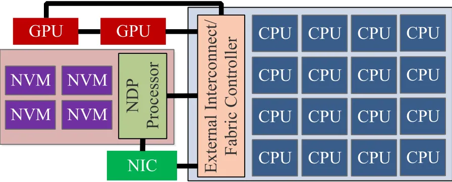
Chapter 5 LEVERAGING NDP FOR CHECKPOINT/RESTART . . . 34
5.1 Compute Node with NDP . . . 34
5.1.1 Operation of Multilevel Checkpointing with NDP . . . 35
5.1.2 NDP for Checkpoint Data Compression . . . 38
5.2 NDP Performance Requirements . . . 39
5.2.1 Configuring NDP for Compression . . . 40
5.3 Evaluation . . . 42
5.3.1 Methodology . . . 43
5.3.2 Checkpoint/Restart Overhead Components . . . 44
5.3.3 Progress Rate Comparison . . . 45
5.3.4 C/R Overhead - Breakdown (4% I/O Recovery) . . . 46
5.3.5 C/R Overhead - Sensitivity Study . . . 47
5.4 Summary . . . 49
Chapter 6 PERFORMANCE, POWER AND COST ANALYSIS FOR COMBINATION OF CHECK-POINT/RESTART OPTIMIZATIONS. . . 51
6.1 Introduction . . . 51
6.2 Compression Study . . . 52
6.2.1 Tools and Methodology . . . 53
6.2.2 Data: Compression Speed and Factor . . . 53
6.2.3 Selecting Utility for Checkpoint Compression using NDP . . . 54
6.3 Performance Evaluation . . . 56
6.3.1 Methodology . . . 56
6.3.2 Progress Rate Comparison . . . 57
6.3.3 C/R Overhead - Breakdown (15% I/O Recovery) . . . 58
6.4 Methodology - Cost Analysis . . . 60
6.4.1 Energy Cost . . . 60
6.4.2 Hardware Cost . . . 64
6.5 Results - Cost Analysis . . . 64
6.5.1 Absolute Cost Breakdown . . . 64
6.5.2 Cost Performance Ratio . . . 65
Chapter 7 CONCLUSION. . . 70
LIST OF TABLES
Table 3.1 Exascale system projection scaled from the Titan Cray XK7 supercomputer . . . 14
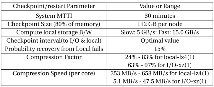
Table 4.1 Checkpoint Data Details. Second column shows the size of total checkpoint data collected for each mini-app in gigabytes. Further columns show compres-sion speed for checkpoint data using different utilities and comprescompres-sion levels on theHDDandSSDsystem. Compression speed is for a single thread of each utility. Value inside () is the compression level. . . 20 Table 4.2 Checkpoint commit and restore time in seconds for all compression utilities.
Checkpoint size for all mini-apps is set to 112 GB per compute node. ‘I/O’ column contains checkpoint times when checkpoints are compressed and saved to global I/O storage. ‘L/S’ and ‘L/F’ contains checkpoint times when checkpoints are compressed and saved to slow compute node local storage (5 GB/s) and fast compute node local storage (15 GB/s) respectively. Note that the checkpoint time values in the “Average" row are not the average values of the seven mini-apps, but the checkpoint time if the performance model is simulated using average compression factor and compression speed from Figure 4.1. Note that checkpoint commit/restore time in the absence of com-pression would be I/O: 1120s, L/S: 22.4s and L/F: 7.47s. . . 22 Table 4.3 C/R parameters for evaluation using performance model . . . 26
Table 5.1 The required compression speed, required number of processor cores in NDP and the smallest possible checkpoint interval to I/O based on average com-pression factor and speed. . . 42 Table 5.2 C/R parameters for evaluation using performance model . . . 44
Table 6.1 Checkpoint compression data. lz4-compressed data of 7 mini-apps is com-pressed again using various compression utilities. The first column shows the size of lz4-compressed checkpoint data used to collect compression parame-ters. Columns with header ’F’ contain compression factor and columns with header ’S’ contain compression speed in MB/s. Compression speed is the speed at which lz4-compressed data is compressed using various utilities. . . . 52 Table 6.2 Cumulative or equivalent checkpoint compression data for compression after
Table 6.3 Checkpoint commit time in seconds for all compression utilities for 2 scenar-ios.UnC: Uncompressed checkpoint data compressed by NDP (Scenario-1); Uncompressed checkpoint size for all mini-apps is set to 112 GB per compute node.Comp: lz4-compressed checkpoint data compressed by NDP ( Scenario-2). Checkpoint size is the size if 112 GB of checkpoint data of the corresponding mini-app is compressed using lz4. Note that the checkpoint time values in the “Average" row are not the average values of the seven mini-apps, but the
check-point time if the performance model is simulated using average compression factor and compression speed from Figure 4.1. . . 55 Table 6.4 C/R parameters for performance, power and cost evaluation of multilevel
LIST OF FIGURES
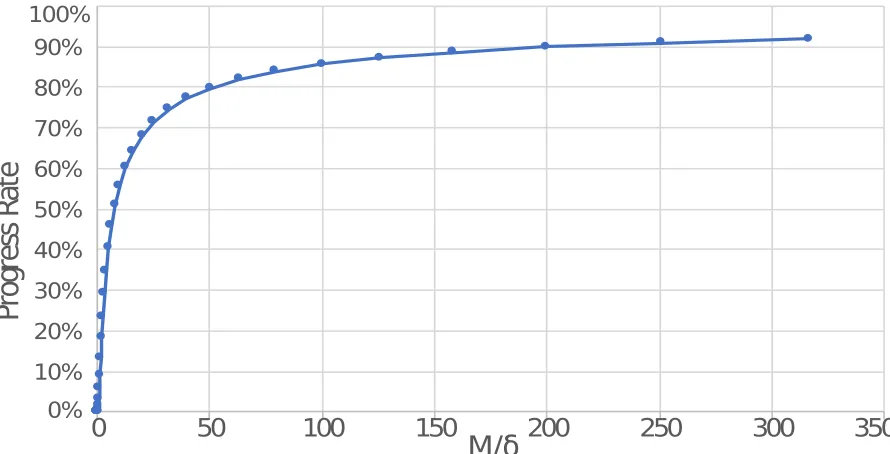
Figure 1.1 Progress rate of a system with C/R as a function ofM/δ. Increasing value of M/δleads to higher progress rate. . . 2
Figure 4.1 Compression factor for checkpoint data of mini-apps using various compres-sion utilities. Value inside () is the comprescompres-sion level. . . 20 Figure 4.2 C/R overhead breakdown for one L/F+I/O-Comp configuration on y-axis
for increasing ratio of locally-saved to I/O-saved checkpoints (n) on x-axis. Note that y-axis does not start at 0 for better resolution. . . 31 Figure 4.3 Frequency of writing checkpoints to global-I/O storage for seven mini-apps
and the average compression case shown as bar plot. On y-axis, frequency of checkpointing is normalized to frequency of checkpointing for no compres-sion case. Total checkpoint I/O write traffic shown as line plot, normalized to checkpoint I/O write traffic generated for no compress case. . . 32 Figure 4.4 Progress rate comparison between different configurations. Data is shown for
7 mini-apps studied and an average progress rate over the 7 mini-apps. For I/O onlythe compression factor and speed corresponds to the xz(1) speed from Table 4.1. Similarly for other configuration for checkpoints to I/O, com-pression factor and speed corresponding to xz(1) is used, while for local level, if compression is performed the parameters corresponding to lz4(1) are used. 32 Figure 4.5 C/R overhead breakdown normalized to compute time(left) and as % of
to-tal execution time(right). Y-axis does not start at 0 for plot on the right. Six configurations from the left: multilevel with no compression (local: 5GB/s), multilevel with compression to I/O (local: 5GB/s), multilevel with compres-sion to both (local: 5GB/s), multilevel with no compression (local: 15GB/s), multilevel with compression to I/O (local: 15GB/s), multilevel with compres-sion to both (local: 15GB/s). The probability that recovery from local fails for multilevel cases: 15%. Compression factor- I/O: 80.6%; Local:64.8% . . . 33
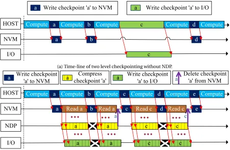
Figure 5.1 Hardware organization of a compute node with our proposed Near Data Checkpointing Architecture (NDCA). . . 35 Figure 5.2 Time-line of multilevel checkpointing with and without NDP. ’HOST’: Primary
processing of compute node+DRAM; ’NVM’: Compute node local storage; ’I/O’: I/O nodes based storage or global I/O. . . 36 Figure 5.3 Ratio of the number of locally saved to the number of I/O saved checkpoints
for different configurations and compression factors . . . 42 Figure 5.4 Progress rate comparison between different configurations. Data are shown
Figure 5.5 C/R overhead breakdown normalized to compute time (left) and as % of total execution time (right). Y-axis does not start at 0 for both plots. Four configura-tions from the left: multilevel (Local+I/O-H), multilevel+compression (Local +I/O-HC), NDP (Local+I/O-N) & NDP+compression (Local+I/O-NC). The probability that recovery from local fails: 4%. Compression factor: 73% . . . 46 Figure 5.6 Progress for five C/R configurations for increasing checkpoint size. Y-axis
does not start at 0%. MTTI: 30 minutes . . . 48 Figure 5.7 Progress for five C/R configurations for increasing MTTI. Y-axis does not start
at 0%. Checkpoint size: 112 GB per compute node . . . 49
Figure 6.1 Progress rate for C/R configurations in which NDP reads lz4-compressed data from node local storage (local-level). Data is shown for 7 mini-apps studied and an average progress rate over the 7 mini-apps. Compression data for compression performed using NDP is obtained from Section 6.2 . . . 59 Figure 6.2 C/R overhead breakdown for C/R configurations listed in Section 6.3.1.2 . . . . 67 Figure 6.3 Five year cost breakdown (in USD) per compute node and progress rate for
C/R configurations listed in Section 6.3.1.2 . . . 68 Figure 6.4 Cost breakdown (in USD). Cost is per compute node per 1018(exa) floating
point operations for C/R configurations listed in Section 6.3.1.2 . . . 68 Figure 6.5 Cost (in USD) per compute node per 1018(exa) floating point operations for
CHAPTER
1
INTRODUCTION
1.1
Overview
Increasing size and complexity of high-performance computing (HPC) systems to achieve exascale performance is projected to cause a decrease in the system mean time to interrupt (MTTI). Check-point/restart (C/R) is a widely used mechanism to deal with failures in HPC systems. It involves saving the state of the application required to resume the application to stable storage at certain intervals. In case of a failure or interrupt, the application’s execution resumes from the most recent checkpoint (saved state). In the absence of C/R, a failure would lead to the application having to restart from the beginning, losing all completed work. However, C/R mechanisms also add perfor-mance overhead due to the time spent saving the checkpoint state, restoring from the saved state, and re-running lost work (work performed since the most recent checkpoint). The efficiency or availability of exascale systems with C/R is projected to be around 50%[Ber08].1C/R efficiency or
progress rate is the ratio of the time it takes to run an application in the absence of failures and C/R overhead to the time it takes to perform the task in the presence of such overheads.
Under some simplifying assumptions, progress rate can be approximated as a function of ratio of MTTI(M) and time to save checkpoint(δ)[Dal06; Dal07].2Figure 1.1 illustrates this function. For
0% 10% 20% 30% 40% 50% 60% 70% 80% 90% 100%
0
50
100
150
200
250
300
350
Pr
og
re
ss
Ra
te
M/
ẟ
Figure 1.1 Progress rate of a system with C/R as a function ofM/δ. Increasing value ofM/δleads to higher progress rate.
exascale systems with checkpoint/restart, this ratio ofM/δdecreases due to two factors. On one hand, the increasing number of compute nodes needed to reach exaflops performance would lead to a decrease in the system MTTI because the MTTI of a single compute node is not improving[SG07]. On the other hand, exascale systems are expected to have larger physical memory capacities and are expected to be able to run applications with larger problem sizes. This will lead to larger application state that needs checkpointing. Without a proportional increase in checkpoint commit write to storage, the time to save checkpoint(δ) will increase. The combination of these two factors leads to a reduction in the ratio ofM/δand thus the progress rate.
I/O or storage hierarchy improves the access time to storage by means of having fast intermediate levels between compute and disk based global I/O. These intermediate levels in the form of burst buffers or compute node local storage can be flash-based solid state drives or SSDs. They provide a lower overhead storage site to stage data by the compute before it is drained to slower disk-based storage in I/O node[Bhi16]. While this alleviates the performance overhead by reducing the access time to storage (including for C/R), moving large data between storage in different levels of hierarchy is not energy efficient. Near data processing (NDP) is effective in reducing the amount of 2While Daly’s work[Dal06]provides an equation to calculate the optimal checkpoint interval given MTTI(M) and
checkpoint commit time (δ),Quantifying Checkpoint Efficiency[Dal07]provides an equation that calculate checkpoint
data movement in many applications by performing computations closer to data. Offloading some application’s computations from the host processors to NDP has shown to improve performance and energy efficiency, especially for data intensive applications[Kan13a; Cho16; Ses14; Do13; Tiw13; Cho13]. NDP (or active storage) can potentially address key challenges in the areas such as scalability, performance, and reliability for I/O systems in exascale computing[Don11]. In this work we show that NDP can be leveraged to improve C/R performance.3
Using SSDs as burst buffer or node local storage would provide a higher bandwidth for writing and reading checkpoints thus decreasing C/R cost. However, using SSDs has been shown to be an expensive way to reduce C/R cost. Ibteshamet al. in[Ibt15]show that it is more cost effective to improve the efficiency of C/R using software techniques such ascheckpoint compression[Ibt15; Ibt12b]orincremental checkpointing[Fer11; Kai16; Nic13]. Based on these observations we evaluate the benefits of combining the use of NDP and checkpoint compression to reduce C/R overhead at a lower cost.
1.2
Existing C
/
R Optimization Techniques
A number of optimizations and mechanisms[Moo10; Di14; Don09; Kan13b; Zhe04; Ben09; Raj13; Ibt15; Ibt12b; Fer11; Kai16; Nic13; Gam14; Ell12; DP12]have been proposed to reduce C/R overhead. While a mechanism likepartial redundancy[Ell12]decreases effective MTTI to reduce C/R overhead, many mechanisms aim to either increase the effective checkpoint commit bandwidth[Moo10; Di14; Don09; Kan13b; Zhe04; Ben09; Raj13]or reduce the checkpoint size[Ibt15; Ibt12b; Fer11; Kai16; Nic13]. Increasing the checkpoint commit bandwidth or decreasing checkpoint size decreases the value ofδ, thus improving the progress rate. Many of the techniques that reduce the effective checkpoint commit time take advantage of the storage hierarchy. Multilevel checkpointing is a clear example of C/R mechanism that exploits storage hierarchy to improve C/R performance.
Multilevel checkpointing[Moo10; Di14]involves writing frequent checkpoints to compute node local storage, while writing occasional checkpoints to global I/O based storage. To keep the overhead of checkpoints to compute node local storage low, the bandwidth of local storage needs to be high. This can be achieved by adding storage in the form of flash based solid state drives (SSDs). The bandwidth requirement and thus the hardware cost for fast local storage would increase with the increasing checkpoint size and failure rate in HPC systems.
Another issue with multilevel checkpointing is the high overhead of the occasional checkpoints 3NDP could be in the context of main memory (like DRAM) or in the context of storage (like SSDs). In this work NDP
to global I/O. Writing a checkpoint out to global I/O in a conventional multilevel checkpointing system requires the host processor to read the checkpoint data from main memory, and then send the data over the network to the remote storage, which requires the host to execute all of the code associated with running the full network stack (e.g., TCP/IP). This can be a particularly slow process as the checkpointing process is typically bottlenecked on the slower I/O (disk) bandwidth at the shared remote I/O nodes. While this is happening, the host processor is generally not available to perform the “useful” computations of the main application. While bandwidth of the local storage in compute node scales, that of global I/O based storage does not scale with the increasing size of application. Moodyet al. in[Moo10; Di14]show that with increasing failure rate and increasing time to save checkpoint to global I/O, the progress rate of a system with multilevel checkpointing decreases, although slower than the decrease for single level checkpointing.
1.3
Adding Checkpoint Compression to Multilevel Checkpointing
Multilevel checkpointing increases the effective bandwidth of reading and writing checkpoint data by saving most checkpoints to fast compute node local storage, while saving a few checkpoints to high overhead global I/O based storage. These local storage will have increasing cost due to increasing bandwidth requirement, with increasing checkpoint size and failure rate for HPC systems. In Chapter 4, we show that checkpoint data compression before writing to local storage reduces the bandwidth requirement for local storage. The high performance overhead associated with checkpointing to global I/O is also mitigated by compressing checkpoint data before writing to global I/O. While, adding checkpoint compression to multilevel checkpointing is an intuitive (or obvious) solution to mitigate issues with scaling of multilevel checkpointing for exascale system, in this work, we study how compression can be added to multilevel checkpointing. We evaluate the compression performance requirement to add compression at all levels of multilevel checkpointing and provide a methodology as to how the requirements can be determined. In Chapter 4 and Chapter 6 we quantify the performance and cost efficiency improvement for multilevel checkpointing due to the addition of checkpoint compression. Our evaluation shows that even with the addition of compression to each level of multilevel checkpointing, the overhead associated with checkpointing to global I/O is still high and provides further opportunity for improvement.
1.4
Leveraging NDP to Improve C
/
R Efficiency
storage (i.e., storage with different speeds and availability at different levels in hierarchy). We propose leveraging additional feature of hierarchical storage - the likely presence of NDP or active storage in (future) HPC systems. Using NDP (i.e., compute capabilities coupled to compute-node local storage) allows the host processor to quickly write checkpoints to the node-local storage and resume execution; NDP can then handle the slower process of sending the checkpoint(s) to global I/O off of the main application’s critical path.
NDP can be leveraged for additional optimizations that improve C/R performance. We explore the benefits of adding compression capabilities to our NDP-based checkpointing scheme, as this can reduce network bandwidth requirement for sending checkpoints out to I/O (thereby reduc-ing network contention for the main application’s communication needs), and it can also help improve performance by speeding up checkpoint restoration (which is primarily limited by how fast checkpoints can be retrieved from the I/O nodes’ disks). While checkpoint compression is not new, the exploitation of an NDP architecture to offload it from the host processor is a new twist: past approaches tolerated higher host-side processing costs because the compression reduced the I/O cost sufficiently to make it a net win, whereas our approach can get the benefits of compression without the host-side overheads.
1.5
Contributions
We make the following contributions:
• We perform a high-level analysis of existing checkpoint/restart optimizations using our pro-jected exascale system. This analysis includes determining the scaling required by these optimizations to achieve a 90% progress rate on our projected system.
• We discuss how checkpoint compression can be added to multilevel checkpointing. Specifi-cally, based on a compression study of checkpoint data, we determine which general purpose compression utilities are best suited to be used with different levels in multilevel checkpointing based on their compression factor and speed.
• We describe the operational details of the checkpoint/restart mechanism using NDP as well as the compute-node’s hardware organization to implement such a mechanism. We evaluate checkpoint compression using NDP as a starting point for exploring additional optimizations that can be performed by NDP.
• We perform a compression study to help select a compression utility that achieves a good trade-off between compression speed and compression factor when compressing checkpoint data using NDP. The study also informs us of the compression speed requirement for the NDP hardware.
• We perform a detailed evaluation of multilevel checkpointing with NDP support. With our proposed NDP approach for offloading I/O management and compression, the host processor is able to increase its progress rate from 51% to 78% (i.e., a more than 50% speedup in the application performance).
• We present a methodology to estimate the 5 year cost of an exascale node for different C/R configurations with certain simplifications. This cost analysis helps compare the cost efficiency of various C/R configuration for our projected exascale node.
1.6
Organization of This Thesis
The rest of the thesis is organized as follows. In Chapter 2 we cover the background and related work to the topics discussed in this thesis. We start by projecting a exascale system configuration in Chapter 3. In this chapter we also project parameters relevant to checkpoint/restart and discuss the limitations of basic checkpoint/restart for our projected exascale system.
In Chapter 4, we discuss our first proposal - adding checkpoint compression to each level of multilevel checkpointing. We discuss how this combination can be achieved in Section 4.1.3. We perform a checkpoint compression study to mimic compression performance for an exascale node with fast local storage (i.e.when compression is not bottlenecked by storage bandwidth) in Section 4.2. Based on this compression study we discuss how a compression utility can be picked for a particular level in multilevel checkpointing in Section 4.2.3. The performance gains of such combination of checkpoint/restart schemes are quantified in Section 4.3.
performance requirement of NDP for scenarios in which NDP is to be used for compression. The impact of leveraging NDP on C/R overhead is evaluated in Section 5.3.
Chapter 6 presents a discussion on how our first two proposals can be combined. In this chapter we discuss how compression requirements for NDP are impacted due to addition of compression at all levels of multilevel checkpointing. In Section 6.3, the performance overhead of the combination of our two approaches is evaluated. Next, in Section 6.4 energy and hardware cost analysis methodology for C/R configurations is described. Finally, in Section 6.5, the cost efficiency data for the various C/R configurations discussed in this thesis is presented.
CHAPTER
2
BACKGROUND AND RELATED WORK
2.1
Checkpoint
/
Restart
Checkpoint/Restart is a widely used fault tolerance mechanism to mitigate the performance over-head of faults in high performance computing systems. Checkpoint/Restart involves saving the state of the application execution periodically. In case of a fault or a failure requiring recovery, application is resumed from the most recent checkpointed state. This avoids restarting the application from the start which would have a high performance cost.
2.1.1 Coordinated Checkpoint/Restart
2.2
Checkpoint
/
Restart Overhead
The increase in C/R overhead for exascale system can be attributed to an increase in failure rate (or decrease in system mean time to interrupt) and an increase in checkpoint size without a corre-sponding increase in checkpoint read/write bandwidth. The following subsections look at each of these aspects.
2.2.1 Failure Rate
Projections show that the system MTTI of exascale machines could be in the range of minutes to tens of minutes[Don11; Ber08; Chu12]. Bergmanet al.[Ber08]project the system MTTI to be 35 minutes - 39 minutes for the strawman exascale system that they project. Chunget al.[Chu12] project the system MTTI to be less than 10 minutes for exascale systems. A study by Schroeder and Gibson[SG07]on petascale systems introduced in 2002-2004 showed ~0.2 failures per socket per year. This is equivalent to a 5 year mean time to failure (MTTF) per socket. This node failure rate has been used in many prior studies[Rie10; Ibt15]to calculate the system failure rate. Using this node failure rate an exascale system with 100,000 nodes would have a system MTTI of 26.28 minutes. This is a more than 5x increase in failure rate compared to a petascale system’s MTTI (which is in the range of hours[Gam14]).
2.2.2 Checkpoint Size
With increasing computational capacity of exascale system, these systems would be able to handle bigger workloads with bigger memory footprint. Therefore these systems are projected to have larger system memory. The total system memory is projected to be in the range of tens to hundreds of petabytes[Don11; Ber08; Chu12]. Since a large part of system physical memory may need to be checkpointed for some applications, the checkpoint size for such applications would also be in the range of tens to hundreds of petabytes. This is a more than 10x increase in system memory compared to petascale systems, none of which have total system memory exceeding two petabytes.
2.2.3 Progress Rate or C/R Efficiency
increasing failure rate (or decreasing MTTI) and increasing checkpoint size for exascale systems, the checkpoint read/write bandwidth would need to increase in proportion to both the increase in fail-ure rate as well as the increase in checkpoint size. This is based on Daly’s formula for calculating C/R efficiency[Dal07]. According to Daly’s formula C/R efficiency is proportional to the system MTTI(M) and inversely proportional to the time to save checkpoint(δ) or C/R efficiency is proportional to M/δ. Time to save a checkpoint (δ) can be approximated as being proportional to checkpoint size (Si z e) and inversely proportional to write bandwidth (B W). Note that we are ignoring the cost of synchronization operation, which would have an increasing cost with increasing number of nodes that need to be synchronized. With this simplification, the C/R efficiency or progress rate is proportional to
M×Si z eB W
. To maintain this ratio, time to save a checkpoint (Si z eB W ) should reduce in proportion to MTTI. This would meanB W should increase in proportion to the increase inSi z e and inversely proportional toM (or directly proportional to failure rate). Based on the projections for exascale system, the I/O bandwidth is not expected to scale in proportion to failure rate and checkpoint size.
2.3
Checkpoint
/
Restart Optimization Techniques
Traditional checkpoint/restart involves periodically saving the state of an application to I/O based storage. In case of a failure, the checkpoint data is used to restore the application and resume its execution from the checkpoint. However increasing failure rate requires proportional decrease in checkpoint commit time to avoid a decrease in progress rate. This would require a decrease in checkpoint size or increase in checkpoint commit bandwidth. The checkpoint size of HPC systems is expected to increase with increasingly large memory footprint of the application. Therefore check-point commit bandwidth need to increase to not only compensate for the increasing checkcheck-point size but also for the increasing checkpoint size failure rate. However, the projected increase in I/O bandwidth is unlikely to be enough to compensate for these effects and therefore to keep C/R feasible[Fer12]for future HPC systems (exascale systems), optimizations or techniques that reduce C/R overhead are increasingly important. While there are techniques[Ell12]that improve C/R performance by increasing the MTTI, most optimizations improve C/R performance by reducing checkpoint commit time. These optimizations can be broadly divided in two categories.
2.3.1 Increase Checkpoint Commit Bandwidth
checkpoint-ing[Moo10; Don09; Kan13b; Zhe04; Gam14], burst-buffers[Bhi16]and file-systems optimized to support faster checkpointing[Raj13; Ben09].
Multilevel checkpointing techniques[Don09; Kan13b; Zhe04; Gam14]are some variation of multilevel checkpoint scheme described by Moodyet al.[Moo10]where checkpoints are frequently saved to faster compute node local storage and less frequent checkpoints are stored to slower global I/O. The compute node local memory could be DRAM[Moo10; Zhe04]or non-volatile memory NVM[Don09; Kan13b]. While the bandwidth to local storage is expected to scale with checkpoint size, the bandwidth to global I/O is not expected to scale[Fer12]. Moodyet al.[Moo10]show that while multilevel checkpointing performs better than single level checkpointing for increasing failure rate and increasing time to save checkpoints to I/O, its performance still reduces. Therefore the global I/O component of multilevel checkpointing will increase with increasing cost of checkpointing to I/O.
These techniques involve saving most checkpoints to a combination of fast and local storage and saving a few to slow disk based storage.
2.3.2 Reduce Checkpoint Data Size
Another set of optimizations reduce the checkpoint commit time by reducing the amount of check-point data that is saved. Example of such optimizations are checkcheck-point compression[Ibt15; Ibt12b], incremental checkpoints[Fer11]and data deduplication[Kai16; Nic13]. Checkpoint compression involves compressing checkpoints using general purpose compression utilities like gzip before saving them. Incremental checkpointing involves creating a full checkpoint followed by saving checkpoint increments which basically involves only saving the states that have changes since last checkpoint. These solutions have been shown[Ibt15]to be cost effective ways of reducing C/R overhead compared to techniques that require hardware support such as fast SSD based storage.
2.4
Near Data Processing
CHAPTER
3
SCALING STUDY
3.1
Overview
In this chapter we project an exascale system configuration starting with an existing petascale HPC system. This projections in turn are used to project the MTTI of an exascale system. The exascale system configuration and the MTTI are used to calculate the overhead of basic C/R with no optimization using Daly’s formula. We use the exascale configuration projected in this chapter to estimate the overhead of various C/R configurations using our performance model throughout this thesis.
3.2
Exascale System Projection
implication of this preference is that we project a conservative increase in physical memory size and, consequently, the checkpoint size. Similarly compared to other projections a conservative increase in failure rate is projected. These assumptions lead to an optimistic scenario for checkpoint/restart cost.
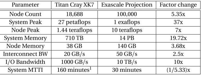
In this study, we scale the Titan Cray XK7 system[Rog12], a petascale system, to exaflops per-formance. Titan has 18,688 compute nodes each consisting of a 16-core AMD Opteron processor coupled with additional GPU acceleration. Each node has a 38 GB of memory (2 GB per CPU core plus the GPU’s 6 GB). Each node has a theoretical peak performance of 1.44 teraflops with a theoret-ical system peak performance of 27 petaflops. A ~37x factor increase is required to reach exaflops performance. This can be accomplished by a combination of increase in performance per compute node and an increase in the number of compute nodes. We assume that the performance of a single compute node can scale to 10 teraflops[Van08], a ~7x increase compared to Titan’s per-node performance. We assume a uniform 7x increase in both CPU and GPU performance. For the CPU, the performance increase is assumed to be achieved by a combination of a 75% increase in performance per core and an increase in core count from from 16 to 64. If the ratio of 2 GB/core is maintained, the memory for the CPU would increase to 128 GB. We conservatively assume that the memory of the GPU is doubled to 12 GB (and not increased 7x, proportional to performance). The total memory for the node would be 140 GB. This is a conservative estimate compared to projections made in past work[Don09]. With a 7x increase in the compute node’s performance, the remaining increase in performance comes from a 5.3x increase in node count (37x/3x). This leads to 100,000 compute nodes, which at 10 teraflops each, provide a system peak performance of 1 exaflops. With 100K compute nodes, the total memory of the system would be 14 PB, again a conservative projection compared to other projections[Don11; Chu12; Don09]. The aggregated data bandwidth of Titan to its file system is 1000 GB/s. We project this to increase to 10 TB/s, a 10x increase which is in the same order as projected by Chen[Che11]. Titan uses the Gemini interconnect which has an injection bandwidth of 20 GB/s. We scale it to 50 GB/s[Che11].
3.3
MTTI Projection
Table 3.1 Exascale system projection scaled from the Titan Cray XK7 supercomputer
Parameter Titan Cray XK7 Exascale Projection Factor change
Node Count 18,688 100,000 5.35x
System Peak 27 petaflops 1 exaflops 37x
Node Peak 1.44 teraflops 10 teraflops 7x
System Memory 710 TB 14 PB 19.72x
Node Memory 38 GB 140 GB 3.68x
Interconnect BW 20 GB/s 50 GB/s 2.5x
I/O Bandwidth 1000 GB/s 10 TB/s 10x
System MTTI 160 minutes1 30 minutes (1/5.33)x
application state, and thus system MTTI would also be ~26.28 minutes. For the sake of simplicity we make an optimistic assumption of system MTTI being 30 minutes for this exascale system, which falls in the range projected in previous work[Chu12]. Key parameters of our projected exascale system are listed in Table 3.1.
3.4
Checkpoint
/
Restart Overhead with no Optimization
This section discusses the feasibility of the overhead of basic C/R for our projected exascale system and the system MTTI. Assuming that 80% of the main memory needs to be checkpointed, each checkpoint would have a size of 11.2 PB for our projected system. Writing a single checkpoint to global file system would require 18.67 minutes at 10 TB/s. Using Daly’s equation[Dal07]to calculate the progress rate, we get a value of 13.67%.2We validated this value using our performance model described in Section 4.3.1.1. This implies that the system will spend more than 85% of the time performing C/R related tasks. How can we improve the progress rate of this system? If we only consider basic C/R without optimization, to achieve a progress rate of say 90% on a system with MTTI of 30 minutes, the required checkpoint commit times comes to 9 seconds (calculated using the same formula used to calculate progress rate given system MTTI and checkpoint commit time). This would require a checkpoint commit rate of (11.2 PB/9 seconds) 1.244 PB/s for the system. This comes to ~12.44 GB/s per compute node. The 1.244 PB/s far outpaces the projected 10 TB/s of global I/O bandwidth, thus requiring additional C/R optimizations.
1Prior work[Gam14]reports 9 failures per day for Titan, which converts to failure every 160 minutes.
2While Daly’s work[Dal06]provides an equation to calculate the optimal checkpoint interval given MTTI and
CHAPTER
4
MULTILEVEL CHECKPOINTING WITH
COMPRESSION
4.1
Introduction
4.1.1 Overview
In this chapter we evaluate the benefits of combining multilevel checkpointing with checkpoint compression. Before that we discuss how these two optimizations can be combined. In the next section, we start by discussing multilevel checkpointing, how it reduces C/R overhead and its limitations with our projected exascale system.
4.1.2 Multilevel Checkpointing
RAMDisk). However this approach does not provide resiliency against a variety of failure modes (temporary loss of power to the DRAM) that non-volatile storage can handle. Future HPC systems are expected to have some non volatile compute node local storage[Kan13b]. For instance, NVM express (NVMe) based solid state drives (SSDs) can be coupled to each compute node to achieve a high aggregate bandwidth. Considering the read/write bandwidth of commercially available SSDs, multiple banks of SSDs may be required to achieve a 12.44 GB/s bandwidth. For e.g., the Seagate Nytro XP7200 drive, has a sequential write speed of 3600 MB/s[Sea]and four such drives in parallel connected using PCIe-3 interface could provide 14.4 GB/s of write bandwidth.
However, storing checkpoints locally in the compute node is not sufficient as the checkpoint data stored may become inaccessible. Therefore in multilevel checkpointing, redundancy is introduced in the form of storing checkpoint data in multiple nodes’ local storage (partner-level) and storing it in global I/O or parallel file system (I/O-level). Thus system can recover from failures frompartner -level orI/O-level when they cannot recover fromlocal-level. Assuming that one can achieve a checkpoint read/write time of 9 seconds forlocal/partnerlevel by coupling high bandwidth SSDs to each compute node, the efficiency of multilevel C/R is still hurt due to the overhead to save (a few) checkpoints to global I/O. In the previous section we mention that it takes ~18.67 minutes to save checkpoints to I/O. If checkpoints are only infrequently stored remotely to defray the high cost of writing a single checkpoint, this will result in higher recovery costs because the checkpoint on an average would have been taken further back in execution, causing the application to have to rerun more work (the work since the last I/O checkpoint and the point of failure). We discuss these conflicting overheads in checkpoint interval and C/R overhead in Section 4.3.2 and demonstrate them in Figure 4.2. In addition adding multiple banks of high bandwidth SSDs which would need periodic replacement would incur a recurring high hardware cost. Therefore more needs to be done to reduce the cost of multilevel checkpointing while limiting its overhead.
4.1.3 Adding Checkpoint Compression to Multilevel C/R
Checkpoint compression[Ibt15]reduces the C/R overhead by reducing the checkpoint write and read time. Prior work has shown that checkpoint data can be compressed effectively using general purpose compression utilities. For instance, work in[Ibt12a]showed that checkpoints could be compressed to as little as 10% of their original size using pbzip2. But a reduction in checkpoint size would not necessarily reduce the overall time to commit checkpoint to storage, if the time to compress checkpoint data exceeds the time saved from writing reduced amount of checkpoint data. Checkpoint compression only helps when the time it takes to compress and write a compressed checkpoint is less than the time it takes to write an uncompressed checkpoint. While the analysis in[Ibt15], serializes the task of checkpoint compression and writing of compressed checkpoint data, in this work we assume that these tasks can be overlapped or pipelined. Therefore checkpoint commit time would be the maximum of the time to compress checkpoint data or the time to write compressed checkpoint data. With this assumption checkpoint compression is beneficial as long compression speed is greater than the write bandwidth to storage and the size of compressed checkpoint data is smaller than uncompressed checkpoint data.
Let’s look at the compression speed requirement in more detail. For multilevel checkpointing, the write bandwidth to storage varies for different levels in the hierarchy. We projected an aggregated I/O bandwidth of 10 TB/s for our exascale system. This implies a 100 MB/s bandwidth per compute node when writing toI/O-level. Therefore a compression rate exceeding 100 MB/s per compute node would reduce checkpoint commit time. This speed can be achieved based on the compression speed analysis in prior work as well as our compression study in Section 4.2. For e.g., we can get a rate of 320 MB/s using 64 compression threads (on 64 CPU cores of our projected compute-node) with a per thread rate of 5 MB/s which is easily achievable.
4.2
Compression Study
We perform the compression study using methodology similar to the one used in[Ibt15; Ibt12b]. We measured compression speeds for multiple utilities using a single compression thread on two different system configurations. The first configuration used for measuring compression speed is a 64-bit Intel Core i7-4770HQ CPU running at 2.2 GHz, with 1600 MHz 16 GB DDR3 memory, running MacOS. This system has a PCIe-based SSD (flash storage). This system with SSD would be a more accurate proxy for the compression speed expected when writing checkpoints to high bandwidth compute node local storage versus a compression study on a system with disk based storage. This is because checkpoints are read from main memory (DRAM) and written to node local storage and therefore should not be bottlenecked by disk storage’s bandwidth. Since we are not certain if the prior checkpoint compression studies (like by Ibteshamet al. in[Ibt15]) were performed on a system with fast SSDs, we do not directly use compression data from prior work. Also the compression speeds that we obtain in this study exceed the values reported in[Ibt15]which could be due to this difference in the hardware used for compression study. For reference we also conduct the study on a second configuration - a 64-bit Intel Core i7-3770 CPU running at 3.40GHz with 1600 MHz 8 GB DDR3 memory. This system has a SATA HDD. For simplicity the first configuration is referred to as SSDand the second asHDD.1
4.2.1 Tools and Methodology 4.2.1.1 Checkpoint data collection
We use seven mini-apps from the Mantevo project[Her09]. They are CoMD version 1.1, HPCCG version 1.0, MiniAero version 1.0, miniFE version 1.5, miniMD version 1.2, miniSMAC2D version 2.0 and pHPCCG version 0.4.CoMDis a reference implementation of typical classical molecular dynamics algorithms and workloads. It is given a 160×160×160 problem size.HPCCGis a simple conjugate gradient benchmark code for a 3D chimney domain on a arbitrary number of processors. It is given a 200×200×64 problem size.miniAerois a mini-app for evaluation of programming models and hardware. It is an explicit unstructured finite volume code that solves the compressible Navier-stokes equations. It is given a 64×64×16 problem size.miniFEis a finite element mini-app which implements a couple of kernels representative of implicit finite-element applications. It is given a 480×320×320 problem size.miniMDis a parallel molecular dynamics simulation package. It is given a 128×128×96 problem size.miniSMAC2Dis an incompressible Navier-Stokes flow solver.
1Even though we collect the compression data for bothSSDandHDDconfiguration, we only use the data for theSSD
It is given a 5k×5k problem size provided along with the mini-app.pHPCCGis related to HPCCG, but has features for arbitrary scalar and integer data types. It is a given a 200×200×64 problem size. These mini-apps are run on a single compute node. The compute node is a 2-way SMP with AMD Opteron processors with 8 cores per socket (16 cores per node) and 2GB memory per core. We use checkpoint/restart support (Berkeley Lab Checkpoint/Restart[Due05]) integrated in OpenMPI framework[Hur07]. Berkeley Lab Checkpoint/Restart (BLCR) library provides support for transpar-ent coordinated checkpoint/restart implementation. The transparent checkpoint/restart technique does not require changes to the application source code, making it convenient for collecting check-point data on applications without checkcheck-point/restart support. Each application is run with 16 MPI processes using OpenMPI[Gab04]version 1.3.3. We take three checkpoints from each application at approximately 25%, 50% and 75% of the execution time. The input sizes for the mini-apps are selected such that the physical memory usage per MPI process fits in the available physical memory per core while giving a good variation of checkpoint sizes across the mini-apps. We observe that the checkpoint size is close to the actual memory usage of the application. Table 4.1 shows the total size of all checkpoint data (in gigabytes) generated for each application.
4.2.1.2 Compression utilities
The compression utilities used for the study are gzip, bzip2, xz and lz4. Each of these utilities has a configurable compression level that ranges from zero/one to nine where a lower values gives faster execution but lower compression factor. For each compression utility except lz4 we use two compression levels: the default level and compression level one. For lz4 we just use the default compression level which is compression level one. The default compression level of a utility is supposed to give the best compression speed and compression factor trade-off for that utility. Below is a brief overview of each compression utility used.
• gzip: gzip is a compression utility which is based on Deflate algorithm [Deu]. Deflate performs compression using a combination of loss-less data compression algorithm LZ77[ZL06]and Huffman encoding[Huf52]. The default compression level is six.
• bzip2[Sew07]: bzip2 compresses data using Burrows-Wheeler transform, which converts frequently-recurring character sequences into strings of identical letters followed by applying move-to-front transform and Huffman encoding. The default compression level is nine.
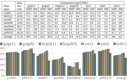
Table 4.1 Checkpoint Data Details. Second column shows the size of total checkpoint data collected for each mini-app in gigabytes. Further columns show compression speed for checkpoint data using different utilities and compression levels on theHDDandSSDsystem. Compression speed is for a single thread of each utility. Value inside () is the compression level.
Data Size (GB)
Compression speed MB/s
Mini- gzip(1) gzip(6) bzip2(1) bzip2(9) xz(1) xz(6) lz4(1)
Apps HDD SSD HDD SSD HDD SSD HDD SSD HDD SSD HDD SSD HDD SSD
CoMD 25.07 64.3 153 65.2 92.3 32.2 32.5 32.0 30.4 35.4 23.5 7.9 8.2 82.3 658
HPCCG 45.92 71.1 150 49.7 61.6 5.0 5.9 4.0 4.6 32.5 47.5 7.0 7.4 77.5 447
miniFE 52.31 49.6 84.5 13.5 24.1 8.3 10.7 8.2 10.1 18.4 18.3 1.9 1.6 52.8 253
miniMD 23.94 41.3 52.2 26.4 27.7 9.6 10.0 10.6 9.2 11.7 8.0 3.2 2.5 52.6 345
miniSmac 28.11 29.0 37.3 21.6 24.4 6.4 6.9 5.6 6.0 10.3 5.1 3.0 2.6 51.2 342
miniAero 0.78 113 138 53.1 61.2 11.1 12.0 7.6 8.2 37.9 28.4 4.4 4.3 366 567
pHPCCG 46.18 43.3 154 52.7 63.2 5.8 6.8 4.5 4.8 59.5 45.9 7.3 7.0 45.7 477
Average 31.76 58.9 110 40.3 50.6 11.2 12.1 10.4 10.5 29.4 25.3 5.0 4.8 104 441
0% 20% 40% 60% 80% 100%
CoMD HPCCG miniFE miniMD miniSMAC miniaero pHPCCG Average
gzip(1)
gzip(6)
bzip2(1)
bzip2(9)
xz(1)
xz(6)
lz4(1)
Figure 4.1 Compression factor for checkpoint data of mini-apps using various compression utilities. Value inside () is the compression level.
• lz4: lz4 is based on LZ77 compression algorithm. lz4 provides high speed compression at the cost of lower compression factor. lz4 compression has many implementations but they all produce output using the same compressed block format[Col11]. The default compression level for lz4 is one.
For each utility and compression level, we measure the compression speed (MB/s) and compres-sion factor on the collected checkpoint data. Comprescompres-sion factor is calculated as
1−u n c o m p r e s s e dc o m p r e s s e d_s i z e_s i z e
.
4.2.2 Checkpoint Compression Speed And Factor
that bzip2 and xz, regardless of the compression level, have an average CPU utilization of ~100% when executed on bothHDDandSSDconfiguration. This indicates they are compute bound. Gzip and lz4 have an average ~100% CPU utilization onSSDbut not onHDD, indicating that gzip and lz4 are I/O bound onHDDconfiguration. This is reflected in the significantly slower compression on HDDcompared toSSDfor gzip and lz4. As discussed in Section 4.2, the compression speed achieved onSSDgives a good approximation of the expected compression speed per thread in our system. The average compression speed onSSDsystem varies from 441.9 MB/s for lz4 (compression level one) to 4.8 MB/s for xz(compression level six).
Figure 4.1 shows the compression factor of checkpoint data for each mini-app using four com-pression utilities. Similar to data for comcom-pression speed, it shows the comcom-pression factor when compression is performed using the default compression level of each utility as well as compression level one. The average compression factor for the utilities varies from 64.75% for lz4(1)2to 83.25% for xz(6).
Table 4.2 Checkpoint commit and restore time in seconds for all compression utilities. Checkpoint size for all mini-apps is set to 112 GB per compute node. ‘I/O’ column contains checkpoint times when checkpoints are compressed and saved to global I/O storage. ‘L/S’ and ‘L/F’ contains checkpoint times when checkpoints are compressed and saved to slow compute node local storage (5 GB/s) and fast compute node local storage (15 GB/s) respectively. Note that the checkpoint time values in the “Average" row are not the average values of the seven mini-apps, but the checkpoint time if the performance model is simulated using average compression factor and compression speed from Figure 4.1. Note that checkpoint commit/restore time in the absence of compression would be I/O: 1120s, L/S: 22.4s and L/F: 7.47s.
Mini- gzip(1) gzip(6) bzip2(1) bzip2(9) xz(1) xz(6) lz4(1)
4.2.3 Selecting Utility for Checkpoint Compression
For the exascale system projected in Section 3.2, the compression data collected above helps us determine which compression utility to use for each level of checkpointing in multilevel check-pointing and the compression performance requirement. In Section 4.1.3, we derived the lower limit of compression speed required per compression thread for the two levels of checkpointing i.e. I/O-level andlocal-level. We also derived the effective time to commit a checkpoint when checkpoint compression and writing of compression checkpoint is overlapped as
m a x
c o m p r e s s i o n t i m e,c k p t s i z ec o m p r e s s e d w r i t e B W
This equation is equivalent to a bottleneck analysis of a pipeline which performs checkpoint com-pression and writing of compressed checkpoint data. This equation can be used to determine the checkpoint commit time for each mini-app and compression utility (and compression level) pair. Also if one conservatively assumes the decompression speed equal to compression speed and read bandwidth of the storage equal to its write bandwidth, the checkpoint restore time would be equal to checkpoint commit time. Note that this is a pessimistic assumption, since generally decompression speed of these utilities is greater than their compression speed and read bandwidth of a storage is greater than its write bandwidth. Table 4.2 shows the checkpoint commit time (same as checkpoint restore time), for each mini-app. We show the data for three different storage, a I/O based storage (I/O) with a bandwidth of 100 MB/s per compute, a fast local storage (L/F) with a bandwidth of 15 GB/s and a slow local storage (L/S) with a bandwidth of 5 GB/s per compute node.
We evaluate the progress rate with both theselocal-level configurations (L/F: local-fast at 15 GB/s; L/S: local-slow at 5GB/s) in Section 4.3.
For theI/O-level, the uncompressed checkpoint commit time is 1120 seconds. The minimum per thread compression speed required to improve this time is (100MBps/64) 1.56 MB/s. All compression utilities have a higher compression speed for all mini-apps and therefore using any of them is an improvement on the checkpoint commit time of the uncompressed case. However, xz(1) gives the smallest checkpoint commit time for all mini-apps forI/O-level, as highlighted in Table 4.2. Methodology similar to the one discussed in this section can be used to pick the best compression utility for each level in multilevel checkpointing based on the bandwidth of the storage in that level.
4.3
Evaluation
In this section we evaluate the impact of adding checkpoint compression to multilevel checkpointing methodology on the performance overhead of our projected exascale system for two hardware configurations. We use progress rate as the metric to compare performance overhead.
4.3.1 Methodology
4.3.1.1 Checkpoint/restart Performance Model
MTTI, checkpoint size and aggregated checkpoint read/write bandwidth. Evaluating performance of multilevel checkpointing requires both compute local storage and global-I/O storage bandwidth. It also requires the probability that recovery from locally-saved checkpoints fails and the number of checkpoints saved to compute node local storage before one is saved to global-I/O.3For analysis of checkpoint compression, checkpoint compression factor and compression speeds for both levels of checkpointing are the inputs to the model. We validated this model for single level checkpointing matching its output with Daly’s model[Dal07].
4.3.1.2 Checkpoint/Restart Configurations
We evaluate the following configurations using the performance model:
1. I/O Only: It is a single level checkpointing scheme where all checkpoints are saved to global-I/O based storage. The data collected is for scenarios with and without checkpoint compression (xz(1)).
2. L/*+I/O: It is a two level checkpointing scheme where most checkpoints are saved to compute node local storage and “one in n" checkpoint is saved to I/O based storage. The optimal value ofnis obtained empirically(see Section 4.3.2). After a failure an attempt is made to first recover from locally-saved checkpoint, but if it fails, it is recovered fromI/O-level. The probability of successful recovery from locally-saved checkpoints is set to 85% based on the observations by Moodyet al. in[Moo10]. The bandwidth of local storage is either 5 GB/s which is referred to asL/S(local-slow) or bandwidth is 15 GB/s denoted asL/F(local-fast).
3. L/*+I/O-Comp: It is a two level checkpointing scheme similar toL/*+I/O. The only difference is that checkpoint data compressed using xz(1) is written toI/O-level. Data written tolocal -level is left uncompressed. Recovery also works similar toL/*+I/O, with the addition of decompression when restoring fromI/O-level.
4. L/*-Comp+I/O-Comp: In this scheme, checkpoint data is compressed before writing to both localandI/Olevel. Checkpoint data is compressed using lz4(1) forlocal-level while xz(1) is used forI/O-level.
3In evaluation, locally-saved checkpoints orlocal-level represent checkpoints saved to compute node local storage
in a single node and redundantly on multiple nodes, thus referring to both thelocalandpartnerlevel of multilevel
Table 4.3 C/R parameters for evaluation using performance model Checkpoint/restart Parameter Value or Range
System MTTI 30 minutes
Checkpoint Size (80% of memory) 112 GB per node Compute local storage B/W Slow: 5 GB/s; Fast: 15.0 GB/s Checkpoint interval(to I/O & local) Optimal value Probability recovery from Local fails 15%
Compression Factor 24% - 83% for local-lz4(1) 63% - 97% for I/O-xz(1) Compression Speed (per core) 253 MB/s - 658 MB/s for local-lz4(1)
5.1 MB/s - 47.5 MB/s for I/O-xz(1)
4.3.1.3 Checkpoint/Restart Parameters
We project exascale system parameters in Section 3.2 and summarize in Table 3.1. Parameters specific to C/R are again shown in Table 4.3. Two configurations for node local storage read/write bandwidth are evaluated - fast local storage (L/F) with a bandwidth of 15 GB/s and slow local storage (L/S) with a bandwidth of 5 GB/s.
The optimalcheckpoint interval, i.e. the time an application performs application’s computation between two checkpoints, is calculated using Daly’s equation[Dal06]. This is the checkpoint interval in case of single level checkpointing. However, for multilevel checkpointing we use this interval for checkpoints tolocal-level which are the more frequent checkpoints. After everyncheckpoints to local, one checkpoint is stored toI/O-level. The optimal value ofnto minimize C/R overhead is determined empirically. The next subsection discusses the impact of varyingcheckpoint interval andnon different components of C/R overhead.
4.3.2 Checkpoint/Restart Overhead Components
We break down the total execution time of an application with C/R into four components:
1. Compute time: Total time spent by an application doing useful work.
2. Checkpoint time: Total time spent by an application to save all checkpoint data. Note that we ignore the synchronization time for coordinated checkpointing, since it will be the same for all configurations studied.
4. Rerun time: Total time spent by an application in rerunning from a checkpoint to the point of failure (equivalent to progress lost from aborting non-checkpointed work).
Components 2-4 are the components of C/R overhead, whereascompute timeis the time it would take to execute an application without C/R overhead in absence of failures. Given the time to commit a single checkpoint and the system MTTI, optimalcheckpoint intervalto minimize C/R overhead can be calculated using Daly’s estimate[Dal06]. Taking checkpoints too frequently results in a higher checkpoint timeas more checkpoints are saved. On the other hand it results in a lowerrerun time, because on an average less work is lost. Taking checkpoints too infrequently has the opposite impact. At the optimal checkpointing interval the total overhead which is the sum of these overheads, is minimum.
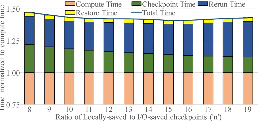
For the multilevel checkpointing scheme, the frequency of I/O-saved checkpoints has a similar impact. Since thecheckpoint intervalfor I/O-saved checkpoints is an integer factor ofcheckpoint intervalfor locally-saved checkpoints (one I/O-level checkpoint everynlocal-level checkpoint), the value ofnhas a similar impact on checkpoint overhead as thecheckpoint interval. Figure 4.2 shows the impact of changing this rationfor aL/F+I/O-Compconfiguration. Figure 4.2a shows the breakdown of total execution time into the four components normalized to compute time while Figure 4.2b shows percentage breakdown of the same. We see in these figures that as the value ofn increases, i.e. as checkpoints to I/O are increasingly less frequent relative to local, the contribution of checkpoint timedecreases but that ofrerun timeincreases. Overall, C/R overhead initially decreases with increasing value ofn, reaches a minimum and then increases for increasing value ofn.
Figure 4.2b shows the same behavior in terms of progress rate. The progress rate initially increases with increasing value ofn, reaches a maximum value, and then decreases. For simulations in this work corresponding to all multilevel checkpointing configurations (with and without compression), the optimal value ofnand thus the frequency of checkpointing to I/O is derived empirically.
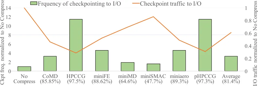
The bar plot in Figure 4.3 shows the optimal checkpointing frequency to I/O for the seven mini-apps as well as for the average compression factor. The frequencies are normalized to the frequency of checkpointing to I/O for the “no compress" case. The value of the compression factor is put along side the mini-app name on the x-axis. The figure shows that the higher the compression factor the higher is the frequency of writing checkpoints to I/O. The bigger the compression factor, the smaller is the checkpoint size and thus the smaller is the overhead for saving a checkpoint. This allows for a higher checkpointing frequency which results in a decrease inrerun time. Thus the optimal frequency of checkpointing increases with higher compression factor.
total time spent saving checkpoints or thecheckpoint timecomponent of the overhead will reduce. This also shows that the increasing checkpointing frequency to I/O will not lead to a higher I/O write traffic, which would have increased the energy cost.
4.3.3 Progress Rate Comparison
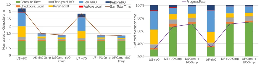
Figure 4.4 shows a comparison of progress rate for three C/R configurations -I/O Only,L/*+I/ O-CompandL/*-Comp+I/O-Comp. The multilevel configurations are evaluated with a slow local storage (L/S: 5 GB/s) and a fast local storage (L/F: 15 GB/s) configuration. For fairness, each mini-app is sized such that they have the same checkpoint size. Each mini-mini-app has different compression factors and compression speeds for both levels (xz(1) for I/O and lz4(1) for local) that are obtained from Table 4.1. As expected, the progress rate is higher for applications with higher compression fac-tor, configurations with faster local storage and for configurations where compression is performed at both levels. On an average, the progress rate increases from 53% forI/O only(with compression) to 66% forL/S+I/O-Comp(multilevel checkpointing with compression for only I/O-level and local storage with 5 GB/s read/write bandwidth). It further increases to 71% when compression is added tolocal-level as well(L/S-Comp+I/O-Comp). On the other hand for fast local storage the progress rates are 71% and 73% forL/F+I/O-CompandL/F-Comp+I/O-Comprespectively. This data shows that on an average, adding compression to I/O-level causes a bigger reduction in progress rate compared to adding compression to local-level. Another observation is that adding compression to local-level forL/F(15 GB/s) configuration only improves the progress rate by 2%. On the other hand, adding compression toL/Sconfiguration has an increase in progress rate by 5%. Another way of looking at the data is that one can reduce the local storage’s read/write bandwidth from 15 GB/s to 5 GB/s by adding compression tolocal-level and maintain the progress rate.L/F+I/O-Comphas the same progress rate asL/S-Comp+I/O-Compof 71% on an average. In the next subsection we look at the breakdown of C/R overhead by the local and I/O component to understand impact of compression on progress rate better.
4.3.4 C/R Overhead Breakdown (by Local and I/O Level)
checkpointing and highlight how compression at each level effects the overhead.
For multilevel checkpointing without compression (L/*+I/O), the plot on the right in Figure 4.5 shows thatrerunoverhead when recovering from I/O (“Rerun I/O”) accounts for more than 25% of the execution time for bothL/FandL/Sconfigurations. This high overhead is due to the low frequency of checkpointing to I/O, which leads to higher amount of lost work. This is in spite of the fact that only 15% of the checkpoints are recovered from I/O. When compression is added to multilevel checkpointing (L/*+I/O-Comp), this component drops to ~10% of the execution time. As discussed earlier, compression of checkpoint data being written to I/O-level reduces the checkpoint commit time to I/O substantially. This leads to writing checkpoints to I/O at a higher frequency and thus reducesreruntime.
The breakdown of C/R overhead forL/F+I/O-Compalso shows that the local components of the overhead are relatively smaller compared to I/O components of the C/R overhead even before checkpoint compression atlocal-level is used. The total C/R overhead associated withI/O-level (i.e. sum ofCheckpoint I/O,Rerun I/O, andRestore I/O) is 18.7% while that associated withlocal-level is 10.3%. Thus a small fraction of checkpoints to I/O (approximately 1 in 10 checkpoints is written to I/O) and a smaller fraction (15%) of recoveries from I/O has a much larger overhead compared to the overhead associated with checkpointing and recovering from local. Thus, there is a potential for further reduction in C/R overhead withI/O-level.
Figure 4.5 shows that checkpoint compression applied tolocal-level only buys a small reduction in C/R overhead. For example, the progress rate improves from 71% forL/F+I/O-Compto 73% forL/F-Comp+I/O-Comp. The figure also shows that the local components of the C/R overhead forL/F+I/O-CompandL/S-Comp+I/O-Compare similar and the overall C/R overhead is similar. Therefore one can use a slower local storage with compression versus a faster local storage without compression to achieve the same progress rate. This would likely lead to a lower hardware cost.
4.4
Summary
In this chapter we evaluated how combining multilevel checkpointing and checkpoint compression reduces C/R overhead. We discussed in detail how these two techniques can be combined, focusing on the compression speed requirement to make this combination beneficial. Our analysis of two level checkpointing (without compression) on a projected exascale system showed that while the overhead for local checkpoints is tolerable, the overhead of checkpoints to global I/O is large. Our evaluation of C/R overhead further shows that adding compression to checkpoints saved to I/O-level leads to a big improvement in progress rate (+30%).