(Under the direction of Professor Peter Bloomfield.)
Value at Risk (VaR) has become a standard measure of risk for financial institutions
as well as central bank regulators. It is used to quantify the total market risk in a
portfolio of financial assets. Hence to estimate VaR accurately is very important. The
definition of VaR is the change in the value of the portfolio of financial instruments with
a given probability over some time horizon. From the statistical point of view, a VaR
estimate is the quantile estimate of the return distribution. This motivates our study of
quantile estimates.
In the application of VaR, most existing models first estimate the whole distribution
and then calculate the quantile. But the characteristics of the financial return distribution
bring extra challenges in distribution estimation. As an alternative to this approach, we
may omit the first step of estimating the distribution and deal with the quantile directly
in a recursive way, as motivated by Engle and Manganelli’s CAViaR model and Tierney’s
Stochastic Approximation estimator.
This dissertation is organized as follows: Part I is an overview of the dissertation.
Part II discusses the recursive way to estimate a quantile of a fixed distribution. A
Smoothed Stochastic Approximation estimator (SSA) has been developed. Part III con-centrates on the approach to track a stochastic quantile. From the work in Part II and
based on the adaptive CAViaR model proposed by Engle and Manganelli and the
expo-nentially weighted stochastic approximation (EWSA) model introduced by Chen,
Lam-bert and Pinheiro (2000), we develop a Hybrid model and an Adaptive Hybrid model
A dissertation submitted to the Graduate Faculty of North Carolina State University
in partial fulfillment of the requirements for the Degree of
Doctor of Philosophy
STATISTICS
Raleigh, North Carolina 2007
APPROVED BY:
Dr. David A. Dickey Dr. Dennis D. Boos
Dr. Peter Bloomfield Dr. Denis Pelletier
Dedication
Chen Ruan was born in April, 1979, in Wuhan City, Hubei Province, China. In 2001,
she received her bachelor’s degree in Industrial Engineering from Wuhan University of
Technology, China. In the fall of the same year, she enrolled in graduate school at North
Carolina State University in the Department of Industrial Engineering. After receiving
her Master of Industrial Engineering, she was thankfully recruited to the Department of
Statistics in 2003. Chen earned her Master of Statistics in 2004 and decided to continue
her study in statistics for her PhD, which would prove to be an excellent decision. She
began working with Dr. Peter Bloomfield during her first year of her doctoral study. She
is completing her Ph.D in the spring of 2007. She will join Capital One at Richmond,
Acknowledgements
My deepest gratitude is due to my advisor Dr. Peter Bloomfield, who has been
pro-viding me tremendous amount of help throughout my research. His brilliant ideas and
remarkable knowledge always inspire me and smooth away my road blocks. His
pro-foundly optimistic attitude to both research and life has been such a great comfort for
me and encouraged me to carry on through hard time. I have been so fortunate to have
him as my advisor. Without him, this thesis would not have been possible.
I would like to thank Dr. David A. Dickey, Dr. Dennis D. Boos and Dr. Denis Pelletier
for serving in my committee. Their insightful suggestions and comments make this work
more complete. I benefit a lot from the interesting courses that they taught, and I also
admire their expertise and devotion to their professional career.
My sincere appreciation also goes to Dr. William Swallow who first recruited me to
the Statistics Department and offered me the invaluable opportunity to continue on my
Ph.D study. I would like to thank him for his guidance and supports when I barely knew
statistics and helped me with his great patience and considerations during my first year
in Statistics Department.
I would like to thank Dr. Pam Arroway for her help in my financial support, Dr.
Leonard Stefanski for his support and supervision, Dr. Jeffrey Thompson for being such
a nice mentor when I first taught the undergraduate statistics class, Mr. Adrian Blue
for his assistance in so many ways, and Mr. Terry Byron for his professional technical
support. My special thanks also go to Drs. Bibhuti Bhattacharyya, John Monahan, Marie
Contents
List of Figures . . . viii
List of Tables . . . ix
I
Overview
. . . 11 Introduction . . . 2
1.1 General Introduction . . . 2
1.2 Literature Review . . . 3
II
Quantile Estimation in a Fixed Population
. . . 82 Stochastic Approximation Estimation . . . 9
3 Smoothed Stochastic Approximation Estimation . . . 13
3.1 Definition . . . 13
3.2 Theory . . . 14
4 Simulation Study. . . 18
5 Summary . . . 22
III
Stochastic Quantile Estimation
. . . 246 Current Approaches Review. . . 25
6.1 EWSA . . . 25
7 Hybrid Model. . . 29
7.1 Motivation . . . 29
7.2 Method . . . 30
7.2.1 Hybrid Model . . . 30
7.2.2 Adaptive Hybrid Model . . . 32
8 Simulation Study. . . 34
8.1 Simulation Experiment . . . 34
8.2 Results and Discussions . . . 38
8.2.1 Relative Mean Squared Errors . . . 38
8.2.2 Relative Bias . . . 40
8.2.3 Snapshot of One Replicate . . . 41
8.2.4 Estimates ofβ1 and Discussion of Computing Difficulties . . . 57
8.3 Summary . . . 63
9 Empirical Application. . . 68
9.1 Historical Data . . . 68
9.2 Backtesting . . . 69
9.2.1 Unconditional Coverage Test . . . 70
9.2.2 Loss Function . . . 71
9.2.3 Duration Based Test . . . 71
9.3 Results and Conclusions . . . 74
IV
Summary
. . . 8510 Conclusions and Future Topics . . . 86
Bibliography . . . 89
Appendices . . . 92
A Proof of Theorem 3.1 . . . 93
B Proof of Proposition 3.1 . . . 95
B.1 Want to show ˆξn−ξGn→0 almost surely . . . 95
B.1.1 Want to showPnk=0Ak converges almost surely. . . 96
B.1.2 Want to showEn is bounded. . . 97
B.1.3 Want to show ˆξn−ξGn →0 almost surely . . . 98
C.2 Want to show (C.2) is true . . . 106
D Theorem and Lemmas Used for Proofs . . . 109
D.1 Lemma 2 of Albert and Gardner (1967) [1] . . . 109
D.2 Kronecker’s lemma . . . 109
List of Figures
8.1 Time t ReMSE and ReBias for GARCH90 . . . 51
8.2 Time t ReMSE and ReBias for GARCH95 . . . 52
8.3 Time t ReMSE and ReBias for GARCH99 . . . 53
8.4 Time t ReMSE and ReBias for IGARCH99 . . . 54
8.5 Time t ReMSE and ReBias for IGARCH95 . . . 55
8.6 Time t ReMSE and ReBias of Adaptive Hybrid and EWSA . . . 56
8.7 True quantiles v.s. time t quantile estimates whenG= 1000 . . . 58
8.8 True quantiles v.s. time t quantile estimates whenG= 5000 . . . 59
8.9 True quantiles v.s. time t quantile estimates whenG= 10000 . . . 60
8.10 True quantiles v.s. time t Adaptive Hybrid quantile estimates . . . 61
8.11 Impact of Gon the objective function . . . 64
8.12 Distribution of 3-fold max ˆβ1s with different δs . . . 65
8.13 Distribution of 3-fold max ˆβ1s v.s. original ˆβ1s . . . 66
9.1 S&P500 returns with 1% and 5% 1-day VaRs . . . 83
List of Tables
4.1 Means and SEs of Standardized MSEs for the 0.75 quantile ofN(0,1) with
10000 replications . . . 20
4.2 Means and SEs of Standardized MSEs for the 0.90 quantile ofN(0,1) with 10000 replications . . . 20
4.3 Means and SEs of Standardized MSEs for the 0.95 quantile ofN(0,1) with 10000 replications . . . 21
4.4 Means and SEs of Standardized MSEs for the 0.99 quantile ofN(0,1) with 10000 replications . . . 21
8.1 Means and SEs of ReMSE of the 0.05-quantile estimates . . . 42
8.2 Means and SEs of ReMSE of the 0.01-quantile estimates . . . 43
8.3 Means and SEs of ReBias of the 0.05-quantile estimates . . . 44
8.4 Means and SEs of ReBias of the 0.01-quantile estimates . . . 45
8.5 Means and SEs of SE of the 0.05-quantile estimates . . . 46
8.6 Means and SEs of SE of the 0.01-quantile estimates . . . 47
8.7 Means and SEs of ˆβ1s (α= 0.05) . . . 48
8.8 Means and SEs of ˆβ1s (α= 0.01) . . . 49
8.9 Summary Statistics for Adaptive Hybrid Model (α= 0.05) . . . 50
8.10 Summary Statistics for Adaptive Hybrid Model (α= 0.01) . . . 50
8.11 Summary of Stripness . . . 63
9.1 Summary Statistics of Backtesting 1-day 5% VaRs for S&P500 . . . 79
9.2 Summary Statistics of Backtesting 1-day 1% VaRs for S&P500 . . . 80
9.3 Summary Statistics of Backtesting 1-day 5% VaRs for the portfolio . . . 81
Part I
Chapter 1
Introduction
1.1
General Introduction
Risk management is one of the most important objectives for all financial institutions.
Risk could be roughly explained as uncertainty of the changes of future returns. Market
risk represents the uncertainty of the future returns due to changes in market conditions.
The direct impact of market risk is that adverse changes in market conditions may result
in severe losses. Other than this aspect, market risk may also lead to the default of a
counterparty and thus impose a credit risk to the other institution. Because of those
facts, market risk is one of the most important aspects of risk management.
Value at Risk (VaR) is used to quantify the total market risk in a portfolio of financial
assets. It has become a standard measure of the market risk for financial institutions as
well as central bank regulators. The Basel Committee on Bank Supervision published
the 1996 Amendment [20], which requires banks to hold capital for market risk as well as credit risk. The Bank for International Settlements (BIS) (1996) calculates the capital
requirements based on VaR estimates.
percentile of the distribution of the change in the value of the portfolio over the next N
days” when N days is the time horizon and X% is the confidence level.
According to Frey and McNeil (2002) [12], the definition of VaR is as follows:
Definition 1.1 Given some confidence level α∈(0,1), VaR at the confidence level α is given by the smallest number l such that the probability that the loss L exceeds l is no larger than (1−α). Formally,
V aRα = inf{l∈R, P(L > l)≤1−α} (1.1)
As we can see, the definition of VaR coincides with the definition of the α-quantile of
the distribution of the loss L. For example, BIS (1996) requires banks to calculate VaR
with N = 10 and α = 0.99; then the VaR is the 0.99-quantile of the distribution of the
losses of the portfolios over the next 10 days. By the connection of the two definitions,
if we could track the quantile, especially the extreme quantile, very accurately, we will
have an accurate estimate of VaR and thus a better control of market risk.
1.2
Literature Review
A natural apporach to estimating a quantile is firstly estimating the distribution of
future returns and then calculating the target quantile. However, the characteristics of
financial data bring exceptional difficulties in estimating the return distribution. The
major empirical facts about financial data can be summarized as follows:
• Financial return distributions are not fixed, but change over time.
period.
All the existing methodologies for calculating VaR try to account for some of the above
features. Examples are RiskMetrics introduced by J.P.Morgan (1996) [14], Generalized
Autoregressive Conditional Heteroscedasticity (GARCH) introduced by Engle (1982) [9]
and Bollerslev (1986) [3], historical simulation, applications of Extreme Value Theory
(see, for example, Danielsson and de Vries (1998) [7]), etc. But criticism exists for all
of them, and the estimates of VaR from different models may be quite different. (See
Manganelli and Engle (2001) [18] for a comparison of VaR models.)
Engle and Manganelli (2004) [10] proposed aConditional Autoregressive Value at Risk (CAViaR) model which skips the issue of modeling the whole distribution and estimates
the quantile directly. Let Y = {yt}Tt=1 be the time series of portfolio returns, and let
qα,t denote the α-quantile of the return distribution at time t. Then a generic CAViaR
specification is :
qα,t =β0+
q
X
i=1
βiqα,t−i+
q+r
X
j=q+1
βjl(yt−j) (1.2)
where p = q+r+ 1 is the dimension of β, which is estimated by regression quantiles,
and l is a function of a finite number of lagged values of observations. Various CAViaR
models are derived by choosing different specifications of l. In Engle and Manganelli
(2004) [10], four variants were introduced, of which the Adaptive CAViaR model is one:
• Adaptive CAViaR:
qα,t =qα,t−1+β1
1
1 +eG(yt−1−qα,t−1) −α
(1.3)
Although Engle and Manganelli (2004) [10] do not give a reference, the adaptive
proposed by Tierney (1983) [24], which is introduced under the framework of stochastic
approximation.
Stochastic approximation was introduced by Robbins and Monro (1951) [22]. They
proposed a recursive way to find the solution x = x0 to the equation M(x) = c, where
c is a constant, and M(·) is a non-decreasing function that can only be evaluated with
error. Letting Xn denote the current estimate of the root x0, we approximate M(·) at
Xn by
Zn+1 =M(Xn) +ǫn+1. (1.4)
Assume ǫn+1 is a random error with mean zero and independent of the previous errors,
Robbins and Monro (1951) [22] proposed to update the estimate of the root x0 by
Xn+1 =Xn+an+1(c−Zn+1) (1.5)
Under some mild assumptions onM(·) and{an},Xn was proved to be consistent forx0.
Sacks (1958) [23] improved the theory and gave the asymptotic distribution of√n(Xn−
x0). Letting an = dn−1, Sacks showed that if M′(x0) = m(x0) exists and 2dm(x0) >1,
then the distribution of√n(Xn−x0) is asymptotically normal with mean zero and
vari-ance d2σ2(2dm(x
0)−1)−1, where σ2 is the variance of the error ǫi.
By a simple calculation, we see that the asymptotic variance is minimized at d =
m−1(x
0). We could estimateM′(x0) bymn based on sample observations and obtain the
modified estimator:
ˆ
Xn+1= ˆXn+dn(n+ 1)−1(c−Zn+1) (1.6)
where dn = m−n1. According to Ventner (1967) [25] and Fabian (1968) [11], under some
additional conditions, √n( ˆXn−x0) converges to a normal distribution with mean zero
sample from M(·); in the above notation, the SA estimator is :
ˆ
Xn+1 = ˆXn−
dn
n+ 1(Z(Yn+1,Xˆn)−c) (1.7)
where Z(Yn+1,Xˆn) = I(Yn+1 ≤ Xˆn) and dn = min( ˆfn(ξ)−1, d0na). Here 0 < a < 12,
d0 >0, ˆfn is the current estimate of the density of X at the α-quantile based on sample
observations. For example, Tierney estimates f(ξ) recursively by the identity ˆfn(ξ) =
1
n
Pn−1
i=0
I(|ξˆi−Xi+1|≤hi+1)
2hi+1 , where the sequence{hn}tends to zero at some appropriate rate.
Tierney’s SA estimator is consistent for x0 and has the same asymptotic variance as the
sample quantile.
Comparing Tierney’s SA estimator (1.7) with Engle and Manganelli’s adaptive CAViaR
model (1.3), we see a resemblance in their structure. Tierney used the indicator function
I(Yn+1 ≤ Xˆn) as the estimate of the function M(·); while the adaptive CAViaR model
used 1
1+eG(yt−1−qα,t−1) and as n goes to infinity,
1
1+eG(yt−1−qα,t−1) →I(yt−1 ≤qα,t−1).
However there is a significant difference between the adaptive CAViaR model and
the SA estimator. The adaptive CAViaR model was developed to track a quantile that
changes over time, while the SA estimator assumed that the distribution of theY is fixed
and thus it estimated a fixed quantile. For the case that data are i.i.d., we place an equal
weight on each individual data point, i.e., the data collected a year ago will have the same
impact as the data came in today on our fixed quantile estimation and asymptotically
the newer data will have negligible weights. But for the stochastic quantile estimate,
the profits and losses that happened one year ago are much less relevant to our quantile
tracking than those that just happened yesterday. So when distribution function changes
This big gap was bridged by research carried out at Bell Lab. In Chen, Lambert and
Pinheiro (2000) [4], a modification was made for the SA estimator and the incremental
Exponentially Weighted Stochastic Approximation (EWSA) was introduced. The EWSA applied exponential weighting in both the quantile estimation and the density estimation
and thus more weights were given to more recent observations.
This thesis starts with fixed quantile estimation developed from Tierney’s work. After
accomplishing satisfactory improvements in the i.i.d. case, we then turn to stochastic
Part II
Quantile Estimation in a Fixed
Chapter 2
Stochastic Approximation
Estimation
In this part, we discuss quantile estimation in a fixed population. Supposed we are
interested in estimating the α-quantile (or the αth percentile) of an unknown but fixed
distribution functionF based on an i.i.d. random sample of size n.
Let X1, X2, . . . , Xn be a random sample from the cumulative distributionF. Denote
the root ofF(x) =α byξ and assumeξ is unique. The most natural candidate is theαth
sample quantile, i.e., the [αn]th smallest of the n observations. It has been shown that,
under some mild restriction on F, the sample quantile is consistent and asymptotically
normal with mean ξ and variance n−1α(1−α)f−2(ξ). Here f(ξ) = F′
(ξ). According to
Pfanzagl (1974) [21], the sample quantile has the smallest asymptotic variance among all
translation invariant estimators of ξ unless we make more assumptions on F.
However, as pointed out in Tierney (1983) [24], computing the sample quantile always
results in a prohibitive requirement of direct access storage space if n is large. Hence
quantile, based on stochastic approximation. The estimator is called Stochastic Approx-imation (SA) estimator which requires only a fixed storage space determined by a batch size that may be as small as 1. Tierney had shown that the SA estimator was consistent
and had the same asymptotic variance as the sample quantile. And an estimate of the
standard deviation of the estimator was also obtained.
Tierney’s SA estimator is defined recursively as:
ˆ
ξn+1 = ˆξn−
dn
n+ 1
ZXn+1,ξˆn
−α (2.1)
where
ZXn+1,ξˆn
=I(Xn+1 ≤ξˆn), (2.2)
dn=min( ˆfn(ξ)−1, d0na), (2.3)
ˆ
fn(ξ) =
1
n
n−1
X
i=0
Iξˆi−Xi+1
≤hi+1
2hi+1
= 1
n
(n−1) ˆfn−1(ξ) +
I(
ξˆn−1−Xn
≤hn)
2hn
,
and
I(x≤y) =
1 (x≤y),
0 (x > y).
Here ˆfn is the current estimate of the density of X at theα-quantile, the sequence {hn}
tends to zero at some appropriate rate, 0< a < 1
density ˆf0 could be set as 0 or estimated from preliminary data. And the initial estimate
of ξ, ˆξ0, could be set as the sample quantile of the prelimary data.
The SA estimator adjusts the previous estimate in a way that the adjustment is
proportional to the difference between the target quantile and the empirical indicator
function that the current observation is less than or equal to the last estimate. The step
size of adjustment is tuned by the density at the quantile: if the estimated density at
the last estimate of the quantile is smaller, we will have a larger step of adjustment. To
prevent “exploding” of the step size, dn is bounded from below; d−01 is usually set as the
interquartile range of the preliminary sample.
Tierney (1983) [24] had shown that under the condition that (1)d0 ≥0, (2) we have a
sequence of{hn}of nonnegative numbers that tend to zero and satisfy P∞n=1(n2hn)−1 ≤
∞, and (3) if some mild restrictions onF have been satisfied, then
ˆ
ξn−→a.s. ξ, (2.4)
ˆ
fn(ξ)
a.s.
−→f(ξ), (2.5)
√
n( ˆξn−ξ)
d
−→N 0, α(1−α)f−2(ξ). (2.6)
And the simulation study in Tierney (1983) [24] showed that the standardized mean
squared errors of the SA estimator and the sample quantile were quite close even for
small sample sizes.
However, the SA estimator involves an indicator function I(Xn ≤ξˆn−1) in the
incre-mental estimation of the quantile. This discrete component will increase abruptness: the
step makes no difference between the observations that are close to the quantile estimate
and the observations that are extremely larger or smaller than the quantile estimate. It
increases the quantile estimates by the same amount regardless of whether the
that a smoothed replacement might improve the performance.
In next chapter, we will propose a Smoothed Stochastic Approximation (SSA) estima-tor and show that the SSA estimaestima-tor also retains the asymptotic properties of the sample
Chapter 3
Smoothed Stochastic Approximation
Estimation
3.1
Definition
Based on Tierney’s SA estimator and motivated by Engle and Manganelli (2004) [10],
we propose our Smoothed Stochastic Approximation (SSA) estimator as follows:
ˆ
ξn+1 = ˆξn−
dn
n+ 1
ZXn+1,ξˆn, Gn
−α (3.1)
where
ZXn+1,ξˆn, Gn
= 1
1 +eGn(Xn+1−ξˆn), (3.2)
dn = min( ˆfn(ξ)−1, d0na) (3.3)
and
ˆ
fn(ξ) =
1
n
(n−1) ˆfn−1(ξ) +
I
ξˆn−1−Xn
≤hn
2hn
values as in the SA estimator.
As we can see,
1
1 +eGn(Xn+1−ξˆn) ≈I(Xn+1 ≤ ˆ
ξn)
for large Gn, provided Xn+1 6= ˆξn. Because of this approximation, we expect that as
sample size goes to infinity, the SSA estimator will have the same asymptotic properties as
the SA estimator, or equivalently, the same asymptotic properties as the sample quantile,
if Gn goes to infinity fast enough.
In next section, we will show that under some mild restrictions on the distribution
functionF and the parameters, our SSA estimator is consistent and has the same
asymp-totic variance as the sample quantile if n−1/4G
n→ ∞ asn → ∞.
Due to the continuity of the component 1
1+eGn(Xn+1−ξnˆ ), we expect that our SSA
es-timator may have better performances in small and moderate sample sizes than the SA
estimator while at the same time retaining the asymptotic properties of the sample
quan-tile. The structure also assures that only a fixed storage space is required for updating
the quantile estimates.
3.2
Theory
We describe our theorem in this section. We will show that under some mild
restric-tions on the distribution functionF and the parameters, our SSA estimator is consistent
and has the same asymptotic variance as the sample quantile if Gn goes to infinity fast
enough.
Theorem 3.1 Let α∈ (0,1), d0 ≥0, ξ0 ∈(0,12), a∈ (0,12). It is given that a sequence {hn}of nonnegative numbers satisfies P∞n=1(n2hn)−1 ≤ ∞. Let F be a distribution
func-tion for which f(x) = F′
(x) exists for all x and is uniformly bounded. Suppose F−1 is
continuous and F′′(·) is bounded. Assume that f(·) is positive at ξ, the unique value of
x such that F(x) =α. Let X1, X2,· · · be a random sample from F and define ξˆn, dn and
ˆ
fn(ξ) by (3.1), (3.3), and (3.4), respectively. Then
ˆ
ξn
a.s.
−→ξ (3.5)
and
√
n( ˆξn−ξ)
d
−→N 0, α(1−α)f−2(ξ) (3.6)
if n−1/4G
n→ ∞ as n→ ∞.
We will prove Theorem 3.1 using the following two propositions.
Proposition 3.1 Suppose that f(ξ) = F′(ξ) exists and is positive and suppose that
E " ∞ X n=1 dn
n+ 1
2#
<∞ (3.7)
and ∞ X n=1 dn
n+ 1
=∞ (3.8)
almost surely.
Then ξˆn almost surely converges to ξ.
Proposition 3.2 Assume all of the assumptions of Proposition 3.1 hold and in addition,
dn converges almost surely to a constant d with 2df(ξ) ≥ 1. Then the distribution of
√
n( ˆξn−ξ) converges to a normal distribution with zero mean and variance d2(2df(ξ)−
1 +eG(x−x)
and define ξG such that
FG(ξG) = α
We write
ˆ
ξn−ξ = ( ˆξn−ξGn)
| {z }
(1)
+ (ξGn −ξ) | {z }
(2)
;
if we could show that both (1) and (2) go to zero almost surely, then we must have ˆξngoes
toξ almost surely. The convergence of (1) can be obtained by modifying the arguments
used to prove Proposition 1 in the appendix to Tierney (1983) [24]. The convergence of
(2) can be shown by first showing the convergence of F(x′) and F
Gn(x′) and then the
convergence of (2) follows because of the assumption that F−1 is continuous.
To prove Proposition 3.2, we show that
√
n( ˆξn−ξGn)
d
−→N 0, d2(2d f(ξ)−1)−1α(1−α) (3.9)
and
√
n(ξGn −ξ)→0 if n
1/4 =o(G
n). (3.10)
Then Proposition 3.2 will be established. Note that when d = f−1(ξ), we have the
asymptotic variance in Proposition 3.2 equal to the asymptotic variance in Theorem 3.1.
The first part (3.9) is a special case of Theorem 2.2 of Fabian (1968) [11]. To prove the
second part (3.10), we define
h(X) =F(X) g(X) = 1
and
Dh =h′
(X) = f(X) Dg =g′
(X) = Ge
GX
(1 +eGX)2
The convolution of Dh and g is
Dh∗g =
Z
f(τ) 1
1 +eG(τ−t) dτ =FG(t)
By applying Differentiation and Commutativity rule of convolution and using a Taylor
Expansion, we will achieve Proposition 3.2.
After proving the two propositions, we then finish our proof of Theorem 3.1 by
ver-ifying the assumptions of the two propositions using the assumptions of Theorem 3.1.
Detailed proofs of Theorem 3.1, Proposition 3.1 and Proposition 3.2 are given in the
Chapter 4
Simulation Study
The three quantile estimators, SA, SSA and sample quantile have been compared in
a simulation study.
We are interested in evaluating how close the three quantile estimators are to the
target 0.75,0.90,0.95 and 0.99 quantiles of a Standardized normal distribution. The
three estimators are compared based on samples of size 50, 100, 200, 500, 1000, 2000,
5000 and 10000. The simulation was replicated 10000 times.
When computing the SSA estimator and the SA estimator , we set the initial estimate ˆξ0
equal to the [10α]th smallest of the first ten observations, d−1
0 equal to the interquartile
range of the first ten observations, ˆf0(ξ) equals zero and a equals 0.45 which is within
(0,1
2). We chose {hn} as
n−1/2 .
The R project function “optimize” was used to chose the best G in the range of (0,50)
with the smallest mean squared error1.
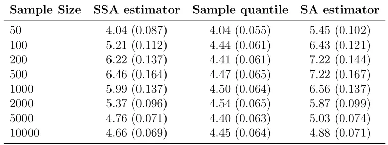
The means and standardized errors of the standardized mean squared errors are listed
in Table 4.1, Table 4.2, Table 4.3 and Table 4.42. The standardized mean squared errors
1
This strategy to choose a bestGcan only be used for a Monte Carlo study.
2
are defined as the mean squared errors of the estimators multiplied by the sample size.
From those results we could see that the SSA estimator outperforms the SA estimator in
all sample sizes for all listed quantiles. Furthermore, the SSA estimators are quite close
to the sample quantiles for most quantiles and in some cases even better than sample
quantiles. The exceptions are for 0.99th quantile, in which the SSA is not comparable to
the sample quantile for sample size equal 500 and larger. But still the SSA has much
Table 4.1: Means and SEs of Standardized MSEs for the 0.75 quantile of N(0,1).
Sample Size SSA estimator Sample quantile SA estimator
50 1.83 (0.029) 1.81 (0.025) 2.19 (0.033)
100 1.83 (0.027) 1.81 (0.025) 2.17 (0.031)
200 1.84 (0.026) 1.84 (0.026) 2.11 (0.030)
500 1.82 (0.026) 1.85 (0.026) 2.03 (0.029)
1000 1.79 (0.026) 1.84 (0.027) 1.97 (0.029) 2000 1.80 (0.025) 1.84 (0.026) 1.93 (0.027) 5000 1.81 (0.025) 1.86 (0.026) 1.93 (0.027) 10000 1.82 (0.025) 1.86 (0.026) 1.91 (0.026)
Table 4.2: Means and SEs of Standardized MSEs for the 0.90 quantile of N(0,1).
Sample Size SSA estimator Sample quantile SA estimator
50 2.99 (0.055) 2.85 (0.040) 3.64 (0.062)
100 3.45 (0.071) 2.90 (0.041) 3.99 (0.076)
200 3.48 (0.065) 2.91 (0.039) 3.95 (0.069)
500 3.24 (0.055) 2.90 (0.041) 3.59 (0.059)
Table 4.3: Means and SEs of Standardized MSEs for the 0.95 quantile of N(0,1).
Sample Size SSA estimator Sample quantile SA estimator
50 4.04 (0.087) 4.04 (0.055) 5.45 (0.102)
100 5.21 (0.112) 4.44 (0.061) 6.43 (0.121)
200 6.22 (0.137) 4.41 (0.061) 7.22 (0.144)
500 6.46 (0.164) 4.47 (0.065) 7.22 (0.167)
1000 5.99 (0.137) 4.50 (0.064) 6.56 (0.137) 2000 5.37 (0.096) 4.54 (0.065) 5.87 (0.099) 5000 4.76 (0.071) 4.40 (0.063) 5.03 (0.074) 10000 4.66 (0.069) 4.45 (0.064) 4.88 (0.071)
Table 4.4: Means and SEs of Standardized MSEs for the 0.99 quantile of N(0,1).
Sample Size SSA estimator Sample quantile SA estimator
Chapter 5
Summary
This part of the study is about estimating a quantile of a fixed distribution.
Through-out Part II, we have assumed that our data are independent and all come from a static
distribution F. The goal of a fixed quantile estimation is to produce the estimate that
would be computed for the entire database. But the sample quantile, the most natural
candidate, requires large memory space. As an alternative, based on Tierney’s work, we
have developed a space-efficient incremental smoothed stochastic approximation
estima-tor that tracks the fixed quantile recursively. It requires only a fixed sestima-torage space, yet
retains the asymptotic properties of the sample quantile.
We have seen that the replacement of the discrete component by the smooth
com-ponent improves the stochastic approximation estimator. And we also have shown by
Theorem 3.1 that asymptotically, the SSA estimator has the same statistical properties
as the sample quantile. From the simulation study, our SSA estimator outperforms
Tier-ney’s SA estimator in all sample sizes and performs closely to the sample quantile for
most sample sizes and quantile values.
This improvement suggests that an extension could be made for the current fixed
estimator update formula. The indicator function was applied in both the quantile
esti-mation and the density estiesti-mation. Since we benefit from replacing the indicator function
with a continuous function in the quantile estimation, we might be able to get another
gain if we replace the indicator function in the density estimation with some continuous
function too. This could be one subject of future study for the fixed quantile tracking.
The work we have done for fixed quantile estimation prepares us for our next subject
of study: stochastic quantile estimation. A stochastic quantile estimation, especially an
extreme stochastic quantile estimation, has a direct application in the VaR calculation.
Unlike the fixed case where data are assumed to be i.i.d., the objective of stochastic
quantile tracking is to estimate a quantile that reflects the current behavior of the data.
Part III
Chapter 6
Current Approaches Review
6.1
EWSA
When we turn to stochastic quantile estimation, out goal has changed to find a value
that describes thecurrent quantile at time t. In order to reflect the current behavior, more weight should be placed on more recent observations. In Chen,Lambert and Pinheiro
(2000) [4], a modification was made for the SA estimator to adapt to stochastic quantile
tracking and the incremental exponentially weighted stochastic approximation (EWSA) was introduced.
Suppose a buffer can hold M observations and at time t the observations are labeled
Xt1,· · · , XtM. TheseM observations come from a distributionFt, which hasαth quantile
qt, i.e., Ft(qt) = α.Theαthquantile is stochastic sinceFt andqtchange over time. Under
this setting, the SA estimator can be considered as a special case thatM = 1 andFt and
qt are constant. In contrast with the SA estimator which gives little weight to new data,
the EWSA estimator applies exponential weighting so that more weight is given to more
recent observations.
1. Set the initial estimate S0 equal to the αth sample quantile of X01,· · · , X0M.
2. Estimate the scale r0 of f0 by the interquartile range of X01,· · · , X0M; i.e.,
by the difference of the 0.75 and 0.25 sample quantiles. And take c0 =
r0M−1PMi=1i−1/2.
3. Take f0 = (2c0M)−1max{#{|X0i−S0| ≤c0},1}, which is the density of
observations in a neighborhood of width 2c0 of S0, unless the fraction of
ob-servations in the neighborhood is zero. Here #{A} is the number of times
that condition A is satisfied.
• The updating equations are:
St(w) =St−1(w)−
w
ft−1(w)
#{Xti≤St−1}
M −α
; (6.1)
ft(w) = (1−w)ft−1(w) + w
2ct−1M
#{|Xti−St−1| ≤ct−1}. (6.2)
Let rt be the difference of the current EWSA estimates for the 0.75 and 0.25
quantiles; the neighborhood size for the next updating step is ct = rt/c, where
c=P2i=MM+1i−1/2/M.
The simulations of Chen,Lambert and Pinheiro (2000) [4] show that the EWSA
out-performs the SA estimates especially when extreme quantiles are tracked for patterns of
behavior that change over time. This is not surprising since SA estimator was originally
6.2
CAViaR
Engle and Manganelli (2004) [10] proposed a conditional autoregressive value-at-risk (CAViaR) model which avoids the issue of modeling the whole distribution and instead
estimates the quantile directly. To reflect the empirical fact that volatilities of
finan-cial returns cluster over time, they incorporate an autoregressive specification into the
quantile modeling.
Let{yt}Tt=1 be the time series of portfolio returns;αis the probability associated with
the target quantile; letSt(β1) denote the time tα-quantile of the distribution of portfolio
returns formed at time t−1. Then a generic CAViaR specification is :
St(β) = β0+
q
X
i=1
βiSt−i(β) +
q+r
X
j=q+1
βjl(yt−j) (6.3)
wherep= 1+q+ris the dimension ofβandlis a function of finite number of lagged values
of observations. Various CAViaR models are derived by choosing different specifications
of l. Among them, the Adaptive CAViaR is defined as:
St(β1) =St−1(β1)−β1
1
1 +eG(yt−1−St−1(β1)) −α
(6.4)
Engle and Manganelli (2004) [10] estimate the parameters of CAViaR models by
regression quantiles, introduced by Koenker and Bassett (1978) [16]. Consider a sample
of observations y1,· · · , yT generated by the model:
yt=S yt−1,Xt−1, . . . , y1,X1;β0
+ǫαt Quantα(ǫαt|Ωt) = 0 (6.5)
≡St β0
+ǫαt, t= 1, . . . , T. (6.6)
whereQuantα(ǫαt|Ωt) is the α-quantile ofǫαt conditional onΩt, Xt is a vector of
exoge-nous variables, β0 is the p-vector of true unknown parameters, and Ω
min
β
1
T
T
X
t=1
[α−I(yt < St(β))] [yt−St(β)]. (6.7)
Engle and Manganelli (2004) [10] proved that the regression quantile estimator ˆβ is
consistent for β0 and asymptotically normal. Analysis of regression quantile models has
been extended to various cases; for example, Komunjer and Vuong (2006) [17] study
Chapter 7
Hybrid Model
7.1
Motivation
Now let’s look at the adaptive CAViaR model:
St(β1) =St−1(β1)−β1
1
1 +eG(yt−1−St−1(β1)) −α
.
The unknown parameter β1 is fixed and the value of the optimal β1 was chosen by the
regression quantile criterion:
min
β1
1
T
T
X
t=1
[α−I(yt < ft(β1))] [yt−ft(β1)].
Let’s turn back to the EWSA estimator:
St(w) =St−1(w)−
w
ft−1(w)
#{Xti≤St−1}
M −α
;
ft(w) = (1−w)ft−1(w) + w
2ct−1M
#{|Xti−St−1| ≤ct−1}.
Our previous study for fixed quantile estimation suggests that we might again benefit
from replacing the indicator function with a continuous function in the EWSA updating
In the EWSA estimator, the fixed parameter w serves as a memory parameter and
ft is the estimate of the density at the quantile. Thus the rate w/ft−1 is linked to the
past memory and at the same time reflects the current behavior of density. Moreover,
the memory parameter w is dimensionless, i.e., the value of w would not be affected
by changing the scale of the data. This property makes it possible to compare w’s for
different sets of data. However, in Chen, Lambert and Pinheiro (2000) [4] the value of
w was set by experiment. In the adaptive CAViaR model, the fixed parameter β1 plays
a similar role as the rate w/ft−1 and thus is not dimensionless. So the optimal β1 for
one set of data might not be the best for the same set of data in a different scale. So
we would like to make β1 dimensionless too. By changing the parameter β1 to fβt−11 to
account for the current behavior of the density function at the current estimate of the
quantile, the newβ1 is now dimensionless and thus will not be changed by changing the
scale of data. After this modification, we could again estimate the new β1 by regression
quantiles.
7.2
Method
7.2.1
Hybrid Model
Let{yt}Tt=1 be the time series of portfolio returns;αis the probability associated with
the target quantile; let St(β1) denote the time t α-quantile of the distribution of returns
formed at time t-1. Based on the adaptive CAViaR model and the EWSA model, we
propose our Hybrid model as follows:
• Initialization:
1. Set the initial estimate S0 equal to the αth sample quantile of preliminary
data.
2. Estimate the scale r0 of f0 by the interquartile range of the preliminary data,
i.e., by the difference of the 0.75th and 0.25th sample quantiles. Let c
0 =r0.
3. Take f0 = (2c0P)−1max{#{|y0i−S0| ≤c0},1}, which is the density of
pre-liminary observations in a neighborhood of width 2c0 ofS0, unless the fraction
of observations in the neighborhood is zero. Here #{A}is the number of times
that condition A is satisfied.
• The updating equations are:
St(β1) =St−1(β1)−
β1
ft−1(w)
1
1 +γαeG(yt−1−St−1(β1)) −α
; (7.1)
ft(w) = (1−w)ft−1(w) + w
2ct−1
I{|yt−St−1(β1)| ≤ct−1}. (7.2)
Let rt be the difference of the current Hybrid estimates for the 0.75th and 0.25th
quantiles; the neighborhood size for the next updating step is ct = 10rt/c, where
c=P2i=MM+1i−1/2/M. Here we have M = 1, soc
t = 10rt/
√
21. Parameters G and
w could again be preset by experiment and we let w= 0.05.
Here we introduce another parameter γα which is itself a function ofα. We useγα to
make sure that we have a positive adjustment whenever the observation yt−1 is greater
than the last estimate of the αth quantile S
t−1(β1) and a negative adjustment whenever
the observation yt−1 is less than St−1(β1), i.e.,
1
1 +γαeG(yt−1−St−1(β1)) ≤α if yt−1 ≥St−1(β1)
1
1 +γαeG(yt 1 St 1(β1))
So we can solve for γα by setting the equation
1 1 +γα
=α. i.e. γα =
1−α α
The unknown parameter β1 will be estimated by regression quantiles:
min β1 1 T T X t=1
[α−I(yt< St(β1))] [yt−St(β1)]. (7.3)
7.2.2
Adaptive Hybrid Model
The parameterGplays an important role in the quantile updating formula. It controls
how fast the continuous component 1
1+γαeG(yt−1−St−1(β1)) converges to its limit, the indicator
functionI(yt−1 ≤St−1(β1)). Gcould not be too large, otherwise we can not benefit from
the continuity; on the other hand, G could not be too small in which case the estimates
are not able to track the changes in distribution of the data. We could treat G as fixed
and decide its value by experiment as we do in our Hybrid model with fixedG; However,
in the situation that the distribution of data changes a lot, for an instance, an IGARCH
distribution, a fixed G is not able to track the dramatic changes. To address this issue,
we develop a variant of the Hybrid model: Adaptive Hybrid model.
The initialization part of Adaptive Hybrid model is identical to the original Hybrid
model. The only differences are in the updating equations.
LetSα,t(β1) denote the time tα-quantile of the distribution of returns formed at time
t-1; the updating equations for Adaptive Hybrid model are:
Sα,t(β1) = Sα,t−1(β1)−
β1
ft−1(w)
1 1 +γαeG
∗
t−1(yt−1−Sα,t−1(β1)) −α
; (7.4)
ft(w) = (1−w)ft−1(w) + w
2ct−1
where
G∗
t =
K
|Sα,t(β1)−S0.5,t(β1)|
. (7.6)
HereS0.5,t(β1) is the estimate of median of the distribution at time t,K is a constant,
other parameters hold the same definitions as in Hybrid model. So instead of setting G
a fixed number, we adjust the value of 1
G∗
t to be proportional to the distance between the current estimates of the target α-quantile and the median. As a comparison, we see that
in Chen, Lambert and Pinheiro (2000) [4], both initialization and updating equations
of EWSA incorporated the parameter rt, which is the interquartile range of the current
estimates, whereas in our Adaptive Hybrid model, we choose the difference between the
Chapter 8
Simulation Study
In this chapter, we investigate the performances of the EWSA, CAViaR and Hybrid
models in quantile estimation for the simulated stochastic populations. We also give
results for the Adaptive Hybrid model when other methods do not perform well.
8.1
Simulation Experiment
In the simulation study, the effects of the Data Generation Process (DGP) are
in-vestigated for the three methods. In addition, the effects of different values of G are
studied for the CAViaR and Hybrid models. Two target quantilesα= 0.05 andα= 0.01
quantiles are considered.
Two kinds of DGPs are considered: GARCH(1,1) and IGARCH(1,1).
• GARCH(1,1):
Proposed by Bollerslev (1986) [3], the equation for GARCH(1,1) is
with
σt2 =a0+a1y2t−1+a2σt2−1, (8.2)
where the innovation ut’s are drawn independently from a standard normal
distri-bution. The long-term variance can be calculated as a0
1−(a1+a2).
By choosing different parameterizations, we have three GARCH(1,1) DGPs as
fol-lows:
1. σ2
t = 1.3333×10⁻⁶+ 0.0667yt2−1+ 0.9σ2t−11,
2. σ2
t = 6.6667×10⁻⁷+ 0.0333yt2−1+ 0.95σt2−1,
3. σ2
t = 1.3333×10
−7+ 0.0067y2
t−1+ 0.99σt2−1.
The initial volatility was set to be 0.0125 and the data are simulated after time 0.
The parameterizations were set so that the long-term variance is 4×10⁻⁵. This
corresponds to a volatility of √4×10−5 = 0.0063, or 0.63%, per day. And a 1 is
two thirds of 1−a2, thus we always have a1+a0 <1.
The GARCH(1,1) DGPs we used here are quite stable. To account for unstable
situations, we also use IGARCH(1,1) DGPs:
• IGARCH(1,1):
Leta0 = 0, a1+a2 = 1, then we have IGARCH(1,1)
yt =σtut
with
σ2t =a1yt2−1+a2σ2t−1
1
1. σ2
t = 0.05y2t−1+ 0.95σt2−1,
2. σ2
t = 0.01y2t−1+ 0.99σt2−1.
According to Nelson (1990) [19], these two IGARCH(1,1) DGPs are both
non-stationary.
In addition to the effects of different DGPs, for CAViaR and Hybrid models that
involve parameter G, we also would like to investigate the impacts of different G values
on the performances of the two methods. We apply our Hybrid model with fixed G
for both GARCH(1,1) and IGARCH(1,1). The strategy we use for the simulation is:
for α = 0.05, we are considering G = 1000, 2000, 3000, 4000, 5000, 10000, 50000 and
1000002. Besides that, for IGARCH(1,1) with a
1 = 0.05 and a2 = 0.95, we also applied
our Adaptive Hybrid model to see how well it will perform under moderate unstable
condition. The values of parameter K we used are K = 10, 20, 30, 40, 50, 100, 500 and
1000; for α= 0.01, we choose G= 1000, 5000, 10000 and K = 10, 50 and 100.3
The total number T of observations per replication equals 3000, corresponding to
around 12 years (255 trading days per year). For each factorial treatment combination,
1000 Monte Carlo replications are generated. A seed is specified and fixed before running
the Monte Carlo simulation for each DGP.
The performance of each incremental quantile estimate ˆSt at time t under each
sce-nario is measured by its empirical time trelative mean squared error(ReM SEt) which is
2
If we multiply the currentytby 100 then we get the return in percentage, in which case the magnitude
ofGwould become 1 percent of the currentGvalues.
3
defined by
ReM SEt=
1 1000 1000 X i=1 ˆ
Si,t−St
St
!2
, (8.3)
whereSt is theα-quantile of the conditional distribution used to generate the data. The
ReMSE at time t is estimated by averaging the squared relative difference between St
and ˆSi,t over the 1000 Monte Carlo simulation runs4.
Therefore, for each method, we have a vector of{ReM SEt}3000t=1 . We can plotReM SEt
v.s. t for the three methods and compare them in the same plot.
We also can compare the performances of the three methods based on their overall relative mean squared error (ReMSE):
ReM SE = 1
1000 1000 X i=1 1 3000 3000 X t=1 ˆ
Si,t−St
St
!2
(8.4)
Similarly, we can calculate a time t relative bias(ReBiast) which is defined by:
ReBiast =
1 1000 1000 X i=1 ˆ
Si,t−St
St
!
(8.5)
and an overall relative bias(ReBias) by
ReBias = 1
1000 1000 X i=1 1 3000 3000 X t=1 ˆ
Si,t −St
St
!
(8.6)
Besides those summary statistics and plots, we can take a “snapshot” at each method,
i.e., pick one replication and picture the estimatedα-quantiles v.s. time. When compared
to the true α-quantiles and the estimated α-quantiles from other methods, we have a
direct idea about how well the model is tracking the true quantiles.
4
8.2.1
Relative Mean Squared Errors
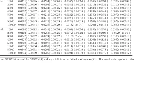
Means and standard errors of the overall relative mean squared errors (ReMSE) for
EWSA, CAViaR and Hybrid models are presented in Table 8.1 forα = 0.05 and Table 8.2
for α= 0.01. For all DGPs except IGARCH95, the Hybrid model has the lowest overall
ReMSEs. The CAViaR model has comparably small overall ReMSEs to the Hybrid model
but all of the ReMSEs are larger than those of Hybrid at each level of G. The EWSA has
largest ReMSEs. The only exception is IGARCH95 of which data are quite unstable: for
α = 0.05, the CAViaR model fails to track the target quantiles, whose smallest ReMSE
atG equaling 5000 is almost two times of that of the EWSA model, not to mention the
big ReMSEs when Gequals 50000 and 100000; The Hybrid model is capable of tracking
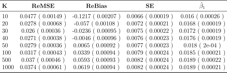
the target quantiles only when G is large (G ≥ 10000); for α = 0.01, both Hybrid and
CAViaR break at each value ofG. For this more unstable IGARCH95 data, we apply our
Adaptive Hybrid model with the results listed in Table 8.9 and Table 8.10. Comparing
the ReMSEs produced by the Adaptive Hybrid model to that of the EWSA, we have a
clear impression that the Adaptive Hybrid model has much smaller ReMSEs and thus
can track the more unstable stochastic quantiles accurately.
As for the G impacts on the ReMSEs of the CAViaR and Hybrid models, we see
that for α = 0.05, the ReMSEs decrease when we increase the G from 1000 to 5000 for
CAViaR and to 10000 for Hybrid, while increase again whenGbecomes larger. A similar
pattern also lies in the case ofα= 0.01. This fact supports our argument thatGcannot
be too small to track the change in the data distribution and at the same time cannot
be too large to gain the benefits of continuity.
G= 1000, 5000 and 10000 in the top panels of Figure 8.1,Figure 8.2, Figure 8.3, Figure 8.4
and Figure 8.5 for different DGPs. From those plots, the ReM SEt of the EWSA model
are always around 0.1 with frequent jumps for all DGPs. For GARCH90 and GARCH95,
we see that ReM SEt of the Hybrid model drops and then jumps back immediately at
the beginning of the data and then quickly stabilizes at low values, the larger the G is,
the quicker it stabilizes. The stabilized value of ReM SEt for G equaling 1000 is clearly
larger than those whenG= 5000 and 10000, but there is little differences in the stabilized
values of ReM SEt between G equals 5000 and 10000. For GARCH99 and IGARCH99
in which case data is changing slowly, ReM SEt of the Hybrid model directly drops to
lower values. The CAViaR has a similar pattern as the Hybrid. The most abnormality
shows up in IGARCH95, where the ReM SEt is far larger than that of the EWSA and is
getting worse till the end of the sample. A larger Gis helpful for bringing the ReM SEt
of the Hybrid model back to a lower level. Both the CAViaR and Hybrid models perform
poorly when compared to the EWSA model for IGARCH95. But when we apply the
Adaptive Hybrid model for IGARCH95, from the top panel of Figure 8.6, we see that
the ReM SEt stabilizes quickly to a low level especially whenK equals 50 and 100.
In summary, in terms of relative mean squared errors, the Hybrid model has the
best performance among all three methods for all DGPs except IGARCH95. When the
simulated data are more unstable, like IGARCH95, the Adaptive Hybrid model can adapt
to the changes in the data more closely and thus achieve smaller ReMSEs and effectively
improve the performances. A moderate value ofGhelps in decreasing the overall ReMSEs
sign as the true target quantile which has a minus sign in our simulation study. Thus a
positive ReBias stands for more conservative of the model, i.e, on average, the estimated
quantiles are smaller than the true quantiles; on the other hand , if the ReBias is negative,
then our estimates are larger than the true quantiles, i.e., the estimates are not extreme
enough.
We have the means and standard errors of overall relative bias (ReBias) represented
in Table 8.3 and Table 8.4. From the Tables, we know that the EWSA model is the most
conservative among all three methods for all DGPs except IGARCH95. For both CAViaR
and Hybrid, the sign of ReBias changes whenGequals 5000 or 10000 in most cases: when
G is comparatively small, the ReBiases are negative since the quantile estimates do not
reflect the changes in the data distribution fast enough, so the quantile estimates are
not extreme enough; while when G is large, the ReBiases are positive since the models
perform more like the EWSA model with discrete component, so the quantile estimates
are more conservative. When looking at the time t relative bias plot at α = 0.05 with
G = 1000, 5000 and 10000 in the bottom panles of Figure 8.1,Figure 8.2, Figure 8.3,
Figure 8.4 and Figure 8.5, similar to the time t relative MSE, the EWSA always has
the ReBias around 0.1 for all DGPs with lots of jumps. Except for IGARCH95, when G
equals 5000 and 10000, the ReBiases of the CAViaR and Hybrid jump to the positive area
and then stabilize around zero; when G equals 1000, the ReBiases rest at the negative
area indicating the updates are not extreme enough whenGis too small. For IGARCH95,
the Hybrid is unable to arrive at a stabilized ReBias value but tends to perform better
when we increase G; the CAViaR always gets a negative ReBias and the absolute value
we use the Adaptive Hybrid model for IGARCH95, the ReBias reaches the area around
zero fast at K equaling 50 and 100.
Therefore, we conclude that the EWSA is the most conservative model in quantile
updating among all methods in the study. It produces the most extreme quantile
es-timates and the value of its ReBias jumps a lot. By choosing an appropriate G, the
Hybrid model has the smallest ReBias with a plus sign, meaning a little conservative.
The Adaptive Hybrid model performs well for IGARCH95 whereas the other models do
not.
8.2.3
Snapshot of One Replicate
In addition to just studying the summary statistics of the three models, it is also
infor-mative to investigate how well the three models perform in one particular replicate, i.e., a
“snapshot” of the simulation. In our simulation study, we choose the 100th replicate and
picture the 0.05-quantile estimates at time t for the three methods with G= 1000, 5000
and 10000 versus the true target 0.05-quantiles along the time in Figure 8.7, Figur 8.8
and Figure 8.9.
As we can see, the estimates from the EWSA model are most variant, jumping most
frequently. This corresponds to the fact that it involves an indicator function in its
updating formula. The CAViaR and Hybrid models produce much smoother lines than
the EWSA. Except for IGARCH95, both CAViaR and Hybrid models track the true
target quantiles more closely when G becomes large while at the same time a larger G
also brings in more variances in the quantile estimates. For IGARCH95, the CAViaR
and Hybrid are not good at tracking the true quantiles especially whenGis small. There
is a plot, laid as the last plot in the bottom panels of above Figures, which is a magnified
Model G GARCH905 GARCH95 GARCH99 IGARCH95 IGARCH99
EWSA – 0.0813( 0.00016 ) 0.0857( 0.00017 ) 0.0982( 2e-04 ) 0.0817( 0.00014 ) 0.0946( 0.00018 )
CAViaR 1000 0.0711( 0.00065 ) 0.0584( 0.00064 ) 0.0365( 0.00054 ) 0.3169( 0.00691 ) 0.0208( 0.00032 )
2000 0.0404( 0.00036 ) 0.0293( 0.00027 ) 0.0186( 0.00023 ) 0.2217( 0.00522 ) 0.0110( 0.00017 )
3000 0.0350( 0.00036 ) 0.0234( 0.00025 ) 0.0142( 0.00019 ) 0.1835( 0.00475 ) 0.0089( 0.00015 )
4000 0.0337( 0.00037 ) 0.0218( 0.00025 ) 0.0128( 0.00018 ) 0.1632( 0.00444 ) 0.0082( 0.00014 )
5000 0.0333( 0.00037 ) 0.0211( 0.00025 ) 0.0122( 0.00018 ) 0.1550( 0.00454 ) 0.0079( 0.00015 )
10000 0.0341( 0.00041 ) 0.0210( 0.00027 ) 0.0120( 0.00018 ) 0.1758( 0.00944 ) 0.0076( 0.00013 )
50000 0.0362( 0.00043 ) 0.0223( 0.00029 ) 0.0129( 0.00019 ) 2.2764( 0.51489 ) 0.0079( 0.00014 )
100000 0.0366( 0.00044 ) 0.0226( 0.00029 ) 0.0132( 2e-04 ) 7.0204( 2.05419 ) 0.0080( 0.00015 )
Hybrid 1000 0.0693( 0.00082 ) 0.0541( 0.00076 ) 0.0304( 0.00056 ) 0.9939( 0.20654 ) 0.0209( 0.00035 )
2000 0.0402( 0.00034 ) 0.0283( 0.00025 ) 0.0172( 0.00024 ) 0.3157( 0.05809 ) 0.0120( 2e-04 )
3000 0.0342( 0.00032 ) 0.0224( 0.00022 ) 0.0132( 2e-04 ) 0.1786( 0.02990 ) 0.0100( 0.00018 )
4000 0.0325( 0.00032 ) 0.0205( 0.00021 ) 0.0119( 0.00019 ) 0.1261( 0.01821 ) 0.0095( 0.00018 )
5000 0.0320( 0.00033 ) 0.0198( 0.00021 ) 0.0113( 0.00018 ) 0.1030( 0.01345 ) 0.0091( 0.00017 )
10000 0.0319( 0.00036 ) 0.0191( 0.00022 ) 0.0111( 0.00019 ) 0.0638( 0.00466 ) 0.0088( 0.00017 )
50000 0.0340( 0.00038 ) 0.0203( 0.00023 ) 0.0119( 0.00019 ) 0.0395( 0.00078 ) 0.0092( 0.00017 )
100000 0.0344( 0.00039 ) 0.0205( 0.00024 ) 0.0121( 0.00019 ) 0.0380( 0.00075 ) 0.0091( 0.00017 )
5
Table 8.2: Means and SEs of ReMSE of the 0.01-quantile estimates.
Model G GARCH90 GARCH95 GARCH99 IGARCH95 IGARCH99
EWSA – 0.0795 ( 0.00056 ) 0.0533 ( 0.00031 ) 0.0482 ( 0.00021 ) 0.4368 ( 0.01221 ) 0.0431 ( 0.00016 )
CAViaR 1000 0.0859 ( 0.0019 ) 0.0706 ( 0.00161 ) 0.0418 ( 0.00083 ) 2.0688 ( 0.13914 ) 0.0267 ( 0.00037 )
5000 0.0566 ( 0.00116 ) 0.0355 ( 0.00078 ) 0.0198 ( 0.00047 ) 0.3289 ( 0.01072 ) 0.0136 ( 0.00029 )
10000 0.0639 ( 0.00126 ) 0.0397 ( 0.00089 ) 0.0221 ( 0.00056 ) 0.7301 ( 0.0385 ) 0.0141 ( 0.00035 )
Hybrid 1000 0.0804 ( 0.00184 ) 0.0655 ( 0.00168 ) 0.035 ( 0.00074 ) 0.2442 ( 0.00969 ) 0.0266 ( 0.00036 )
5000 0.0515 ( 0.00099 ) 0.03 ( 0.00054 ) 0.0159 ( 0.00024 ) 0.3858 ( 0.0124 ) 0.0136 ( 2e-04 )
Model G GARCH90 GARCH95 GARCH99 IGARCH95 IGARCH99
EWSA – 0.0783 ( 0.00046 ) 0.088 ( 0.00048 ) 0.0996 ( 0.00049 ) 0.0903 ( 0.00041 ) 0.0932 ( 0.00047 )
CAViaR 1000 -0.1321 ( 0.00363 ) -0.1099 ( 0.00359 ) -0.079 ( 0.00286 ) -0.3282 ( 0.00679 ) -0.0985 ( 0.00179 )
2000 -0.0812 ( 0.0013 ) -0.08 ( 0.00134 ) -0.0621 ( 0.00131 ) -0.2932 ( 0.00581 ) -0.0581 ( 0.00099 )
3000 -0.0455 ( 0.00099 ) -0.0482 ( 0.001 ) -0.0404 ( 0.00099 ) -0.2268 ( 0.00555 ) -0.0401 ( 0.00084 )
4000 -0.025 ( 0.00094 ) -0.0293 ( 0.00093 ) -0.0245 ( 0.00094 ) -0.1775 ( 0.0052 ) -0.0298 ( 8e-04 )
5000 -0.0123 ( 0.00091 ) -0.0175 ( 0.00089 ) -0.0143 ( 0.00091 ) -0.1385 ( 0.00489 ) -0.0234 ( 0.00078 )
10000 0.0148 ( 0.00091 ) 0.0078 ( 0.00087 ) 0.0076 ( 0.00089 ) -0.0226 ( 0.00381 ) -0.0096 ( 0.00075 )
50000 0.0383 ( 0.00093 ) 0.0299 ( 9e-04 ) 0.0266 ( 0.00087 ) 0.275 ( 0.01609 ) 0.0019 ( 0.00074 )
100000 0.0414 ( 0.00092 ) 0.0328 ( 0.00088 ) 0.0288 ( 0.00087 ) 0.397 ( 0.03141 ) 0.0035 ( 0.00074 )
Hybrid 1000 -0.0713 ( 0.00435 ) -0.0554 ( 0.0039 ) -0.0492 ( 0.00272 ) 0.1292 ( 0.01531 ) -0.0936 ( 0.00193 )
2000 -0.0794 ( 0.00166 ) -0.0742 ( 0.00166 ) -0.0562 ( 0.00143 ) -0.0148 ( 0.0083 ) -0.0581 ( 0.00106 )
3000 -0.0514 ( 0.00108 ) -0.0511 ( 0.0011 ) -0.0405 ( 0.00107 ) -0.0561 ( 0.00601 ) -0.0414 ( 0.00088 )
4000 -0.033 ( 0.00096 ) -0.0355 ( 0.00094 ) -0.0271 ( 0.00096 ) -0.0654 ( 0.00483 ) -0.0315 ( 0.00083 )
5000 -0.0212 ( 0.00093 ) -0.0243 ( 9e-04 ) -0.0181 ( 0.00093 ) -0.0673 ( 0.00429 ) -0.0254 ( 0.00081 )
10000 0.0054 ( 9e-04 ) -3e-04 ( 0.00086 ) 0.0026 ( 0.00088 ) -0.0432 ( 0.00323 ) -0.0126 ( 0.00077 )
50000 0.0292 ( 0.00091 ) 0.0223 ( 0.00086 ) 0.0209 ( 0.00086 ) 0.0249 ( 0.00179 ) -0.0013 ( 0.00076 )
Table 8.4: Means and SEs of ReBias of the 0.01-quantile estimates.
Model G GARCH90 GARCH95 GARCH99 IGARCH95 IGARCH99
EWSA – 0.1229 ( 0.00083 ) 0.0958 ( 0.00071 ) 0.0912 ( 0.00064 ) 0.337 ( 0.00473 ) 0.0761 ( 0.00057 )
CAViaR 1000 -0.0139 ( 0.00559 ) -0.0191 ( 0.00536 ) -0.0371 ( 0.00405 ) 0.3946 ( 0.02358 ) -0.1111 ( 0.00185 )
5000 0.0462 ( 0.00181 ) 0.0193 ( 0.0016 ) 0.0056 ( 0.00133 ) 0.0018 ( 0.00678 ) -0.0126 ( 0.00109 )
10000 0.0798 ( 0.00184 ) 0.0505 ( 0.00165 ) 0.0334 ( 0.00132 ) 0.2299 ( 0.00769 ) 0.0055 ( 0.00112 )
Hybrid 1000 0.0208 ( 0.00519 ) 0.0118 ( 0.00488 ) -0.029 ( 0.0036 ) 0.1052 ( 0.00592 ) -0.1091 ( 0.00182 )
5000 0.0438 ( 0.00177 ) 0.0141 ( 0.00147 ) -0.0041 ( 0.00116 ) 0.2493 ( 0.00649 ) -0.0173 ( 0.001 )
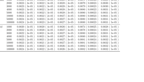
Model G GARCH90 GARCH95 GARCH99 IGARCH95 IGARCH99
EWSA – 0.0039 ( 1e-05 ) 0.0038 ( 1e-05 ) 0.0043 ( 1e-05 ) 0.0093 ( 0.00016 ) 0.0069 ( 3e-05 )
CAViaR 1000 0.0023 ( 3e-05 ) 0.0023 ( 3e-05 ) 0.0028 ( 4e-05 ) 0.0077 ( 0.00023 ) 0.0029 ( 5e-05 )
2000 0.0023 ( 3e-05 ) 0.0022 ( 3e-05 ) 0.0028 ( 3e-05 ) 0.0079 ( 0.00023 ) 0.0030 ( 5e-05 )
3000 0.0023 ( 3e-05 ) 0.0022 ( 3e-05 ) 0.0028 ( 3e-05 ) 0.0079 ( 0.00023 ) 0.0030 ( 5e-05 )
4000 0.0023 ( 3e-05 ) 0.0022 ( 3e-05 ) 0.0028 ( 3e-05 ) 0.0080 ( 0.00023 ) 0.0031 ( 5e-05 )
5000 0.0023 ( 3e-05 ) 0.0022 ( 3e-05 ) 0.0028 ( 3e-05 ) 0.0080 ( 0.00023 ) 0.0031 ( 5e-05 )
10000 0.0024 ( 2e-05 ) 0.0022 ( 2e-05 ) 0.0027 ( 3e-05 ) 0.0080 ( 0.00023 ) 0.0031 ( 5e-05 )
50000 0.0024 ( 2e-05 ) 0.0023 ( 2e-05 ) 0.0027 ( 2e-05 ) 0.0080 ( 0.00023 ) 0.0031 ( 5e-05 )
100000 0.0024 ( 2e-05 ) 0.0023 ( 2e-05 ) 0.0027 ( 2e-05 ) 0.0080 ( 0.00023 ) 0.0031 ( 5e-05 )
Hybrid 1000 0.0020 ( 3e-05 ) 0.0020 ( 4e-05 ) 0.0026 ( 4e-05 ) 0.0074 ( 0.00025 ) 0.0028 ( 5e-05 )
2000 0.0022 ( 3e-05 ) 0.0020 ( 3e-05 ) 0.0027 ( 3e-05 ) 0.0078 ( 0.00024 ) 0.0031 ( 5e-05 )
3000 0.0022 ( 3e-05 ) 0.0021 ( 3e-05 ) 0.0027 ( 3e-05 ) 0.0080 ( 0.00024 ) 0.0031 ( 5e-05 )
4000 0.0023 ( 2e-05 ) 0.0021 ( 3e-05 ) 0.0027 ( 3e-05 ) 0.0080 ( 0.00024 ) 0.0031 ( 5e-05 )
5000 0.0023 ( 2e-05 ) 0.0021 ( 2e-05 ) 0.0027 ( 3e-05 ) 0.0081 ( 0.00024 ) 0.0032 ( 5e-05 )
10000 0.0023 ( 2e-05 ) 0.0021 ( 2e-05 ) 0.0027 ( 2e-05 ) 0.0081 ( 0.00024 ) 0.0032 ( 5e-05 )
50000 0.0024 ( 2e-05 ) 0.0022 ( 2e-05 ) 0.0026 ( 2e-05 ) 0.0082 ( 0.00024 ) 0.0032 ( 5e-05 )
Table 8.6: Means and SEs of SE of the 0.01-quantile estimates.
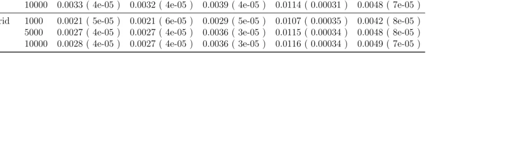
Model G GARCH90 GARCH95 GARCH99 IGARCH95 IGARCH99
EWSA – 0.004 ( 1e-05 ) 0.0039 ( 1e-05 ) 0.0047 ( 1e-05 ) 0.0122 ( 2e-04 ) 0.0072 ( 4e-05 )
CAViaR 1000 0.0025 ( 5e-05 ) 0.0025 ( 5e-05 ) 0.0031 ( 6e-05 ) 0.0105 ( 0.00033 ) 0.0042 ( 8e-05 )
5000 0.0032 ( 4e-05 ) 0.003 ( 4e-05 ) 0.0038 ( 4e-05 ) 0.0115 ( 0.00031 ) 0.0047 ( 7e-05 )
10000 0.0033 ( 4e-05 ) 0.0032 ( 4e-05 ) 0.0039 ( 4e-05 ) 0.0114 ( 0.00031 ) 0.0048 ( 7e-05 )
Hybrid 1000 0.0021 ( 5e-05 ) 0.0021 ( 6e-05 ) 0.0029 ( 5e-05 ) 0.0107 ( 0.00035 ) 0.0042 ( 8e-05 )
5000 0.0027 ( 4e-05 ) 0.0027 ( 4e-05 ) 0.0036 ( 3e-05 ) 0.0115 ( 0.00034 ) 0.0048 ( 8e-05 )
Table 8.7: Means and SEs of β1s for CAViaR and Hybrid (α= 0.05).
Model G GARCH90 GARCH95 GARCH99 IGARCH95 IGARCH99
CAViaR 1000 0.0011 ( 3e-05 ) 7e-04 ( 2e-05 ) 4e-04 ( 1e-05 ) 0.0017 ( 7e-05 ) 8e-04 ( 2e-05 )
2000 0.0013 ( 2e-05 ) 9e-04 ( 2e-05 ) 5e-04 ( 1e-05 ) 0.0021 ( 6e-05 ) 8e-04 ( 2e-05 )
3000 0.0014 ( 2e-05 ) 0.0010 ( 2e-05 ) 6e-04 ( 1e-05 ) 0.0021 ( 6e-05 ) 9e-04 ( 2e-05 )
4000 0.0014 ( 2e-05 ) 0.0010 ( 2e-05 ) 7e-04 ( 1e-05 ) 0.0021 ( 7e-05 ) 9e-04 ( 2e-05 )
5000 0.0014 ( 2e-05 ) 0.0011 ( 2e-05 ) 7e-04 ( 1e-05 ) 0.0021 ( 6e-05 ) 9e-04 ( 2e-05 )
10000 0.0015 ( 2e-05 ) 0.0011 ( 2e-05 ) 7e-04 ( 1e-05 ) 0.0021 ( 7e-05 ) 9e-04 ( 2e-05 )
50000 0.0015 ( 2e-05 ) 0.0012 ( 2e-05 ) 8e-04 ( 1e-05 ) 0.0020 ( 6e-05 ) 9e-04 ( 2e-05 )
100000 0.0015 ( 2e-05 ) 0.0012 ( 2e-05 ) 8e-04 ( 1e-05 ) 0.0020 ( 7e-05 ) 9e-04 ( 2e-05 )
Hybrid 1000 0.0069 ( 0.00026 ) 0.0041 ( 0.00017 ) 0.0021 ( 9e-05 ) 0.0098 ( 0.00015 ) 0.0036 ( 9e-05 )
2000 0.0112 ( 0.00023 ) 0.0071 ( 0.00016 ) 0.0035 ( 9e-05 ) 0.0124 ( 0.00018 ) 0.0039 ( 8e-05 )
3000 0.0119 ( 0.00022 ) 0.0078 ( 0.00015 ) 0.0042 ( 9e-05 ) 0.014 ( 0.00018 ) 0.0039 ( 7e-05 )
4000 0.0124 ( 0.00022 ) 0.0082 ( 0.00014 ) 0.0045 ( 9e-05 ) 0.0152 ( 0.00019 ) 0.0041 ( 8e-05 )
5000 0.0126 ( 0.00022 ) 0.0084 ( 0.00015 ) 0.0047 ( 8e-05 ) 0.016 ( 0.00021 ) 0.0041 ( 8e-05 )
10000 0.0122 ( 0.00019 ) 0.0087 ( 0.00014 ) 0.0051 ( 9e-05 ) 0.0169 ( 0.00019 ) 0.0042 ( 7e-05 )
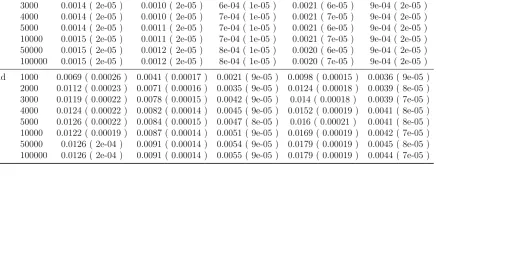
50000 0.0126 ( 2e-04 ) 0.0091 ( 0.00014 ) 0.0054 ( 9e-05 ) 0.0179 ( 0.00019 ) 0.0045 ( 8e-05 )
Table 8.8: Means and SEs of βˆ1s for CAViaR and Hybrid (α= 0.01).
Model G GARCH90 GARCH95 GARCH99 IGARCH95 IGARCH99
CAViaR 1000 0.0023 ( 9e-05 ) 0.0018 ( 8e-05 ) 0.0013 ( 6e-05 ) 0.0051 ( 0.00025 ) 0.0035 ( 9e-05 )
5000 0.004 ( 9e-05 ) 0.0033 ( 7e-05 ) 0.0028 ( 6e-05 ) 0.0074 ( 0.00016 ) 0.0038 ( 8e-05 )
10000 0.0041 ( 8e-05 ) 0.0036 ( 7e-05 ) 0.0031 ( 6e-05 ) 0.0071 ( 0.00016 ) 0.0039 ( 9e-05 )
Hybrid 1000 0.0099 ( 0.00041 ) 0.0083 ( 0.00038 ) 0.0079 ( 0.00037 ) 0.0341 ( 0.00053 ) 0.0161 ( 0.00037 )
5000 0.0223 ( 0.00037 ) 0.0206 ( 0.00035 ) 0.0175 ( 0.00028 ) 0.0374 ( 0.00022 ) 0.0154 ( 0.00025 )
Table 8.9: Summary Statistics for Adaptive Hybrid Model for IGARCH95 (α= 0.05).
K ReMSE ReBias SE βˆ1
10 0.0477 ( 0.00149 ) -0.1217 ( 0.00207 ) 0.0066 ( 0.00019 ) 0.016 ( 0.00026 ) 20 0.0278 ( 0.00068 ) -0.057 ( 0.00108 ) 0.0072 ( 0.00021 ) 0.0168 ( 0.00019 ) 30 0.026 ( 0.00036 ) -0.0236 ( 0.00095 ) 0.0075 ( 0.00022 ) 0.0172 ( 0.00019 ) 40 0.0271 ( 0.00038 ) -0.0046 ( 0.00096 ) 0.0076 ( 0.00023 ) 0.0176 ( 0.00019 ) 50 0.0279 ( 0.00036 ) 0.0065 ( 0.00092 ) 0.0077 ( 0.00023 ) 0.018 ( 2e-04 ) 100 0.0317 ( 0.00043 ) 0.0339 ( 0.00094 ) 0.0079 ( 0.00024 ) 0.0185 ( 0.00021 ) 500 0.037 ( 0.00046 ) 0.0593 ( 0.00093 ) 0.0082 ( 0.00024 ) 0.0189 ( 0.00022 ) 1000 0.0374 ( 0.00061 ) 0.0619 ( 0.00094 ) 0.0082 ( 0.00024 ) 0.0189 ( 0.00021 )
Table 8.10: Summary Statistics for Adaptive Hybrid Model for IGARCH95 (α= 0.01).
K ReMSE ReBias SE βˆ1
G=1000
time
ReMSE
0 500 1000 1500 2000 2500 3000
0.00 0.10 0.20 G=5000 time ReMSE
0 500 1000 1500 2000 2500 3000
0.00 0.10 0.20 G=10000 time ReMSE
0 500 1000 1500 2000 2500 3000
0.00 0.10 0.20 G=1000 time ReBias
0 500 1000 1500 2000 2500 3000
−0.3 −0.1 0.1 0.2 0.3 G=5000 time ReBias
0 500 1000 1500 2000 2500 3000
−0.3 −0.1 0.1 0.2 0.3 G=10000 time ReBias
0 500 1000 1500 2000 2500 3000
−0.3
−0.1
0.1
0.2
0.3
Blue−EWSA; Red−CAViaR; Green−Hybrid
time
ReMSE
0 500 1000 1500 2000 2500 3000
0.00
0.05
0.10
time
ReMSE
0 500 1000 1500 2000 2500 3000
0.00
0.05
0.10
time
ReMSE
0 500 1000 1500 2000 2500 3000
0.00 0.05 0.10 G=1000 time ReBias
0 500 1000 1500 2000 2500 3000
−0.3 −0.1 0.1 0.2 0.3 G=5000 time ReBias
0 500 1000 1500 2000 2500 3000
−0.3 −0.1 0.1 0.2 0.3 G=10000 time ReBias
0 500 1000 1500 2000 2500 3000
−0.3
−0.1
0.1
0.2
0.3
Blue−EWSA; Red−CAViaR; Green−Hybrid