Reconstruction of Ground Penetrating Radar Images using techniques based on Optimization.

(1)

ABSTRACT

SUVARNA, SUSHIL SHEENA. Reconstruction of Ground Penetrating Radar Images Using

Techniques based on Optimization. (Under the guidance of Dr Wesley Snyder and Dr

Leonhard Bernold)

Ground Penetrating Radar (GPR) is an instrument used in semi-automated construction

systems. In principal, images of subsurface objects such as pipes and mines may be detected

and potentially measured. The detection of utilities is complicated by a combination of the

complexity involved in the data collection technique of the GPR and the irregularities present

beneath the surface. This thesis provides the initial results in the development of an algorithm

to invert the effects of these corruptions and return images, which are exact in the placement

and conformation of subterranean objects. The technique employed is a deconvolution-like

method that utilizes a maximum a posteriori (MAP) based optimization method to estimate

the best reconstruction. Mean field annealing (MFA) using gradient descent is the

optimization method used. Using this technique, single objects in the field of observation

were reconstructed to within an acceptable percentage of their original shape. Further work

would involve reconstructing multiple objects in the field of observation as well as

(2)

R

ECONSTRUCTION

O

F

G

ROUND

P

ENETRATING

R

ADAR

I

MAGES

U

SING

T

ECHNIQUES

B

ASED

O

N

O

PTIMIZATION

by

SUSHIL SHEENA SUVARNA

A thesis submitted to the Graduate Faculty of North Carolina State University

in partial fulfillment of the requirements for the Degree of

Master of Science

COMPUTER SCIENCE

Raleigh

2004

APPROVED BY:

________________________ ________________________ Dr Douglas Reeves Dr Mladen Vouk

(3)

BIOGRAPHY

Sushil S. Suvarna was born on December 24, 1979 in the city of Bombay, India. He

completed his Bachelors Degree in Electronics Engineering from Padmabhushan Vasantdada

Patil Pratishthan College of Engineering, Bombay, in May 2001. He then joined North

Carolina State University in Aug 2001, to further a Masters Degree in Computer Science.

During his time at NCSU, he worked on research projects along with Dr L. Bernold and Dr

W. Snyder.

(4)

1. PROBLEM

DESCRIPTION

1.1 INTRODUCTION

Ground Penetrating Radar (GPR) is an instrument that is used for subsurface mapping using

high-frequency electromagnetic waves. We attempt to use this instrument to detect, locate

and measureburied utilities, primarily pipes, both metallic and non-metallic. The first part of

the thesis explains the complex transmitted wave, constructs a model that best represents this

wave, and presents a method based on correlation and thresholding that locates the pipes. The

second half focuses on the signal-spread of the transmitted wave of the GPR, which appears

more as a cone than a single vertical pulse. This spread causes migration of the object, and

we propose a method based on optimization to invert this distortion. Finally, a common

algorithm comprised of the above methods is applied to actual GPR data in real time to

extract all the possible object locations with minimum false positives.

1.2 WHAT IS A GPR?

GPR transmits short pulses of high frequency electromagnetic energy into the ground from a

transmitting antenna. These waves propagate into the ground with a velocity that depends on

the dielectric property of the medium. If the waves encounter an interface between two

materials with different refractive indices, some of the wave energy is reflected back and the

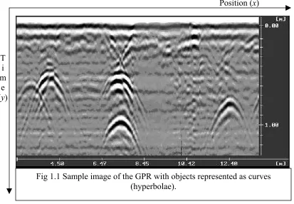
rest continues to propagate to create further reflections. A receiver picks up these reflections

(8)

T i m

e (y)

Position (x)

Fig 1.1 Sample image of the GPR with objects represented as curves (hyperbolae).

In order to create an image, the GPR sends out pulses at a certain frequency and samples the

responses for a certain time slot before recording them as a single column corresponding to a

single position of the GPR. A collection of these columns, representing different positions

recorded in continuance make up an image.

1.3 MATERIAL

CONDUCTIVITY

The type of material in which the waves of the GPR propagate has a strong effect on the

signal penetration and the clarity of the received wave. The different material interfaces that

(9)

in reflection strength, b) changes in arrival time of specific reflections, c) source wavelet

distortion, and d) signal attenuation.

The GPR data consists of a continuous graphic display of reflected energy over a set time

interval. This set time interval is the two-way travel time, measured in nanoseconds. The

depth of the material the wave penetrates can be determined if the velocity of the

electromagnetic energy (ν_m) through the material is known. Using the dielectric constant of

the material, the velocity of the wave can be calculated using the formula

,

r m

c

ε

ν =

where c is the speed of light in vacuum and εr is the dielectric constant of the medium.

Once the speed is known, the depth of a particular object in the image can be calculated by

using the formula

. 2

r m r

t d =ν

dr is the depth, ν_m is the velocity in the medium and tr is the two way travel time from the

GPR to the object.

The penetration depths achieved using the GPR depend on the signal frequency and on the

nature of the material in which it travels. Higher frequency electromagnetic waves give better

resolution, but cannot penetrate to a great depth. Lower frequencies on the other hand

penetrate much deeper but provide poorer resolution. The wave will easily penetrate resistive

materials and will not heavily penetrate conductive materials. Because of their higher

(10)

the technique ineffective. Electromagnetic energy, in these frequency ranges, seldom

penetrates more that 30m into the surface and, in highly conductive material, may only

penetrate a few meters.

1.4 DATA

MIGRATION

Migration is a technique that is used to relocate objects in a GPR image from where they

appear to be, to where they are actually located.

GPR data is misrepresented in two ways, a) due to the structure of the transmitted pulse and

b) due to the spread of the signal of the GPR.

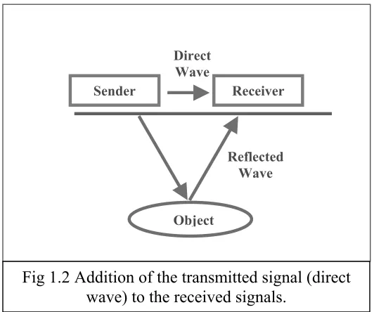
1.4.1 Data misrepresentation caused by the transmitted signal (direct wave)

Fig 1.2 Addition of the transmitted signal (direct wave) to the received signals.

Reflected Wave Direct

Wave

Object

(11)

The receiver of the GPR not only picks up the signals returned by the different objects but

also the direct wave sent out by the transmitter (as shown in Fig 1.2).

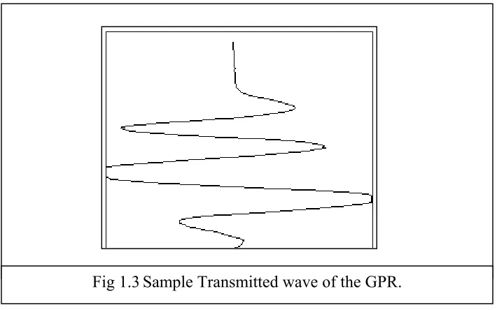
The signal of the GPR (direct wave) is not a simple impulse. It appears similar to a Gaussian

modulated sine wave. The reflections returned from different objects are proportional to

transmitted wave. As the receiver adds the transmitted wave to the returned signals,

understanding the structure of the input wave and its behavior is very important. A sample

transmitted wave is shown in Fig 1.3.

Fig 1.3 Sample Transmitted wave of the GPR.

The alternate positive and negative (left and right) peaks correspond to different intensities of

(12)

The deeper the object, higher the attenuation and lesser the energy that returns. The amount

of energy returning mainly depends on the difference in refractive indices at the material

boundary.

As the observed image g is the result of a convolution between the actual image f and the

input signal s, the relationship is given as

∑

− ×

=

i

i s i y x f y

x

g( , ) ( , ) ( )

where i denotes the number of elements in the input signal s. The x-axis denotes the position

of the GPR and the y-axis denotes time. This convolution is reversed by a technique that uses

the linear correlation coefficient, explained in detail in section 5.1.

1.4.2 Data misrepresentation caused by the signal spread

The GPR transmission is not comprised only of signals transmitted vertically, but rather the

signal spreads out as a cone emanating from the base of the GPR as shown in Fig 1.4.

L

t

Fig 1.4 Signal Spread of the GPR represented as a cone. GPR at (xo,0)

x

(13)

The x-axis represents the movement of the GPR (from the left to the right) along the surface

and the y-axis represents time. The y-axis increases in the downward direction. The same

definition of the x and y axes are maintained for all the images of the GPR.

At a particular position, the intensity of wave reflections from the different objects are

plotted against the distances of the GPR from these objects. Hence the value of a pixel along

the vertical depends on the convolution carried out along the curve of the cone that passes

through this pixel.

∑

+

−

= θ

θ

) , ( ) , ( )

,

(x t f x y h x x t

g _o _o

f is the original image, g is the measured image and h is the kernel The GPR is located at

(xo,0) and remains fixed for one measurement. t denotes time and θ is the angle of spread.

The form of h depends on t, as h is the curve corresponding to a particular value of t. h is

time-variant. Depth (y) and time (t) are interrelated. We measure both of them in the same

units, pixels. For the arc L, all the points lying on the arc are equidistant from the source in

terms of time, but not in terms of depth. Hence during our measurements we need to convert

time into depth. For a fixed position of the GPR (xo,0), the x and y coordinates of the

different points on the arc are given in terms of time t as

. cos

0 t θ

x x= +

. sinθ t y=

where θ is the angle of the signal spread. The model shown in Fig 1.4 is explained in detail in

(14)

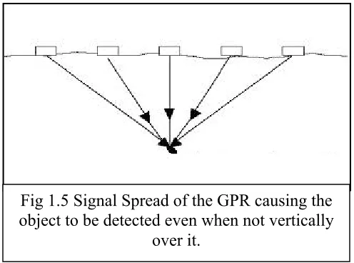
Fig 1.5 Signal Spread of the GPR causing the object to be detected even when not vertically

over it.

Due to the signal spread of the GPR as shown in Fig 1.5, a single object appears as a curve

(hyperbola) as shown in Fig 1.6.

T i m

e (ms)

Position (cm)

Fig 1.6 Hyperbolic representation of an object caused by the signal spread of the GPR.

The shape and size of the hyperbolae created by objects differ based on the location of the

objects. The primary technique used to reconstruct the hyperbolic representations to

(15)

2. LITERATURE

REVIEW

GPRs have been used in a variety of applications including mine detection, utility detection

and mapping, concrete inspection [11] [19] [21] [23], archaeology [12] [20] [24] [33],

structural inspection [2] [6] [10] [15] , geology [1] [16] [17] and mineral detection [8] [9]

[28]. Of these, mine detection has been the most popular topic for GPR research. See [5] [27]

[35] [36] for some recent survey methods. The main advantage of the GPR over other

detectors such as the Electromagnetic Inductor (EMI) is its two dimensional data

representation. In addition to the position of the object, this instrument helps determine its

depth as well.

2.1 GPR ANTENNA CHARACTERIZATION

According to Radzevicius [26], polarization in wave theory describes the magnitude and

direction of electric and magnetic fields with respect to space and time. Two main types of

polarization are linear polarization and circular polarization. If waves are linearly polarized,

the electric field is directed in a straight line from the transmitter (parallel to each other),

whereas in circular polarization the electric vectors emanating from the transmitter are not

parallel to each other.

Radzevicius [26] further states that for spherical targets and most linear targets that include

pipes and cables, the polarization of the reflected field is independent of the transmitted

(16)

antenna and those scattering from the targets. Most modern GPRs use dipole or bow tie

antennas in which the majority of the electric field is incident (moves along) along the long

axis of the bow-tie.

Radzevicius [26] explains that the waves that leave the antenna are called lateral waves and

those already present in the area surrounding the GPR are called space waves. The antenna

patterns observed are considered to be a result of the interference between these lateral and

space waves. However the main factor that defines the antenna pattern is the interaction

between the antenna and the lossy dielectric halfspace that is often very close to the GPR. He

further suggests that the best method to understand the pattern caused by a short dipole

antenna placed near a lossy halfspace is to study the Finite Difference Time Domain (FDTD)

model of the signal spread. Maxwell’s equations are used to model the electric and magnetic

fields of the antenna. FDTD is a method that is used to simulate electromagnetic propagation

[32]. As the electric and magnetic fields can be calculated throughout a discretized volume at

increasing steps of time, the distribution of the electromagnetic fields can be observed as a

function of time. In this case, FDTD was used to replace the spatial and time derivatives in

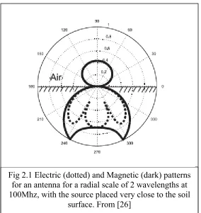
the Maxwell equations with finite difference approximations. His results showed the electric

(17)

Fig 2.1 Electric (dotted) and Magnetic (dark) patterns for an antenna for a radial scale of 2 wavelengths at 100Mhz, with the source placed very close to the soil

surface. From [26]

These lobes, as they are called, caused by the wave interference are heavily dependent on the

frequency of the incident wave. Ideally for most applications the radiation pattern should

contain a single lobe with most of its energy focused in the downward direction. However in

practice, many lobes are created which result in the misrepresentation of data that we

observe. Large numbers of lobes are created at higher frequencies, due to rapid interference

between lateral and space waves, making data interpretation even more difficult.

Daniels [7] also describes antenna characteristics and the various parameters that are

associated with antenna selection. He explains that the major consideration in antenna

selection is the target type and that for most common applications the cross-coupled dipole is

(18)

2.2 CATEGORIZATION OF OBJECT RECONSTRUCTION

TECHNIQUES

Cardimona [4] categorizes the object reconstruction process from raw GPR data into two

parts: “normal processing” and “advanced processing”. Zero time adjust, subtract mean trace

and gain adjustment are included in normal processing. Associating zero time with zero

depth is called zero time adjust. Superposition of the transmitted wave (direct wave) with the

signals received from the ground produces “ringing” or “banding”. A method known a

“subtract mean trace”, which is also a high pass filter, is one way of removing this ringing.

This method takes the average of a window of pixels and subtracts that average from the

value of the pixel that lies in the center of the window. The method is described by the

equation shown below

, ) , ( 1 ) , ( ) , ( 2 2

∑

= − = + −

= i m

m i y i x f m y x f y x g

where m is the window size. This method and the parameters considered in selecting the

window size are described in detail in section 4.2.

Signals that travel less distance and time have greater intensities than the signals that arrive

later. Attenuation of these signals is proportional to the time taken for them to propagate.

This attenuation is caused due to geometric spreading as well as the absorption of energy by

the medium in which the signal propagates. Gain adjustment is required to compensate for

(19)

After the normal or primary processing, advanced techniques can be applied to better

interpret the data, most common of which is “migration”. Migration is one term that is used

to describe the technique of reconstructing the distorted representation of objects in GPR data

(also known as hyperbolae).

The GPR pulse (direct wave) enters the surface and intercepts various irregularities and

convolution is the technique that best describes the interaction of this pulse with these

irregularities. Deconvolution can be used to remove the effects of the direct wave (shaped

like a Gaussian modulated sine wave) to better interpret the GPR image. Inverse filtering is a

kind of deconvolution that is commonly used. Inverse filtering involves taking the Fourier

transform of the distorted signal and removing the distortion using the frequency domain

representation. However, this technique is helpful only when the structure of the source wave

is known. The basic approach to inverse filtering using Fourier transforms is shown below.

), ( * ) ( )

(t f t h t

g =

where g is the observed distortion of a kernel h over the original image f

In the frequency domain this would be represented as (using discrete time Fourier

Transforms)

). ( ) ( )

(k F k H k

G = ×

Deconvolution (inverse filtering) of the original image f in the frequency domain is given as

. ) (

) ( ) (

k H

k G k

(20)

F can be converted back into the time domain using the inverse discrete time Fourier

transform. As the discrete time Fourier Transform (DTFT) is used to represent a

discrete-time non-periodic signal as a superposition of complex sinusoids, the inverse DTFT

representation of a time domain signal involves an integral over frequency namely

ω

π ω

π

d e k F t

f i k

∫

+

−

= ( )

2 1 ) (

2.3 GPRS USED IN MINE DETECTION

Gestel [14], Gader [13] and others have worked extensively in the field of mine detection

using GPRs. Gestel [14] implemented migration using a method called “Alford rotation” that

analyzes “multi-configurational” data to detect the main orientation of the target. By

arranging the receiver and the transmitter in different orientations, data can be recorded in

four configurations and hence the term “multi-configurational data”. Problems with this

method include the requirement to collect data from four angles and the susceptibility of the

algorithm to noise. The noise present in real data causes enough disturbance to make the

algorithm unstable. Also for accurate location using this method, the radiation patterns of the

vertical and horizontal dipoles must be the same, which occurs only in air or extremely

homogenous environments.

In [13], Gader uses Hidden Markov Models (HMMs), stochastic models that produce time

(21)

comprised of landmine signatures derived from multiple sources. This library is the main

platform for the development of the HMM detection algorithm. Using the proposed HMM

technique the algorithm compares a hyperbola with the digital signatures that are present in

the library and generates a probability that’s associated with the best match for that curve.

The HMM technique breaks down the curve into states. Based on the Markov theory that the

probability at each state is only dependent on the previous state, a probability is associated

with each state. This probability attains an acceptable value only if there is a curve,

corresponding to one of the predefined curves, present in the image. The primary

disadvantage of this method is the creation of the signature library. In order to achieve a high

level of accuracy this library must be continually updated with all the possible signatures

from the different objects of interest. Also the various soil types must be taken into

consideration.

2.4 RECONSTRUCTIONS BASED ON OPTIMIZATION

Minimization is a technique used very commonly in image restoration algorithms. Hsiao [30]

presents a method to determine the ultrasonic reflectivity function resulting from density

changes in a medium, which is very similar to the reconstruction of reflections of the

electromagnetic waves in GPR systems. Similar to the problem presented in this thesis, this

paper estimates the reflected wave as a convolution of the input wave and the reflectivity

function of the material. The problem is then reduced to the maximization of a probability

that depends on the variation of the measured image from the unknown, and the prior

(22)

technique called “mean field annealing”, that is a type of optimization that attempts to avoid

local minima. The technique works well for detecting defects in metallic surfaces, however

non-linear reconstructions depend heavily on the prior knowledge of the statistics of the

unknown image.

2.5 ALGORITHMS FOR THE INVERSION OF THE TRANSMITTED

WAVE

In order to reconstruct the received signals that have been distorted due to the convolution

caused by the input wave of the GPR, some models for the transmitted wave have to be

constructed. Van der Lijn [34] has presented models for the input wave and analyzed many

algorithms to generate the impulse response of targets that would make them easier to

classify.

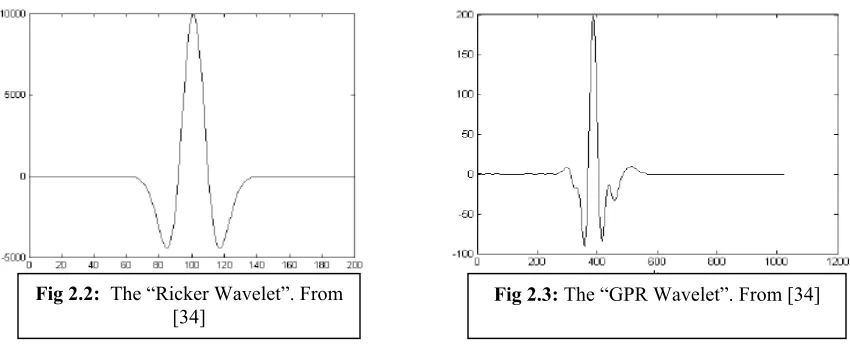
Fig 2.3: The “GPR Wavelet”. From [34]

Fig 2.2: The “Ricker Wavelet”. From [34]

The impulse response of targets gives information about the size, internal structure and

material properties of those targets. In order to obtain the impulse response, many

(23)

wavelet”, shown in figure 2.2, which we observe looks a lot like a Gaussian modulated sine

wave. The second model called the “GPR wavelet”, figure 2.3, was extracted from an actual

GPR signal.

Some of the deconvolution methods employed along with their results are mentioned below.

Deconvolution based on linear least squares uses an error function that is shown below.

2

|| ||

min Xg y

g −

g is an estimate of the impulse response, y is the received signal and the input wave is

represented by X.

After experimentation, Van der Lijn [34], showed that this method worked fine for the “GPR

wavelet” but not for the “Ricker wavelet”. This occurred as to the structure of the “Ricker

wavelet” was smooth with most values being neighbor-dependent unlike the “GPR wavelet”

which had values are independent of its neighbors. The least squares method seems to work

better for waves that had values independent of each other.

A variant of the above method called “ridge regression” is shown below.

) || || || (||

min 2

2 2

2 g

y Xg

g − +λ

The second term calculates the squared second norm of g. This term helps improve the noise

sensitivity during the inversion. The sensitivity to noise is determined by the choice of λ,

(24)

reconstruction. Hence a λ must be selected that provides effective noise reduction and

acceptable errors in the reconstruction.

Van der Lijn [34] also states that by exploiting the structure of the impulse response of the

target, the sensitivity of the deconvolution algorithm to external disturbances could be

reduced. Also only part of the input wave (depending on the type of the wave to decide

which part) plays an important role in the calculation of the output. Hence Van der Lijn [34]

has presented a method called “subset selection using single columns” (SSUSC), which only

tries to use the relevant parts of the input and output waves to help in the reconstruction. The

main advantage of this method is its speed of execution. However, it does require prior

knowledge of the exact shape of the impulse response. Van der Lijn concludes that this is one

of the best deconvolution algorithms and improves on this by presenting variants that help

better determine or select the portions of the wave that need to be dropped.

2.6 MIGRATION

ALGORITHMS

Herman [18] presents an approach that is quite similar to the one we use based on our Ramac

GPR. After eliminating the transmitted wave using a background removal scheme, a

migration technique called “coherent summation migration” is used to relocate the actual

data. This method called volume based processing, uses a summation technique about the

(25)

Fig 2.4: Coherent Summation. From [18]

The principle states that the summation would result in a constructive interference only at the

real locations of the objects and destructive interference elsewhere. An appropriate threshold

decides the presence or absence of an object. The major advantage of this method is that it

can begin even before the data collection is complete.

Herman [18] also describes an alternate method called “surface based GPR processing”

based on template matching that reduces 3D data into 2.5 D. 3D data contains a lot of

information about the soil and the object, some of which might not be required to detect

objects. The transmitted signal of the GPR is structured such that most of the information

from the returned waves is contained at those points of the wave that correspond to large

amplitude or phase changes. Herman states that most of the information in a single received

(26)

the wave through a peak detector, only the peaks remain and the rest of the data is neglected.

This could possibly reduce the number of data points to be observed by a scale of 200. This

new grid of data that only has values at the peaks of the signal is called “2.5 D” data or a

“range image”. By observing the amplitudes of the peaks for the various objects at the

different depths, Herman [18] used template matching and thresholding to detect objects.

Volume based processing is generally poor at handling soil heterogeneities, and requires an

accurate estimate of the velocity in the medium. Surface based processing, on the other hand,

(27)

3. OPTIMIZATION

ALGORITHM

The common algorithm used to invert the distortions produced by the transmitted signal of

the GPR is a technique based on the optimization of an objective function. This objective

function is created by a combination of the data present in the received signal and the known

characteristics of the actual undistorted signal. This function is optimized using a technique

called mean field annealing which uses gradient descent.

3.1 CONSTRUCTING THE OBJECTIVE FUNCTION

In this section I follow the terminology used in [30]. For ease of understanding, we initially

represent the two-dimensional reflectivity function f(x,y) as if it were a one-dimensional

signal f(t). The transformation to two-dimensions is straightforward.

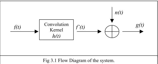
For a linear, time invariant system, we model the generation of the measured signal by the

convolution of an unknown reflectivity function f(t) with a kernel h(t) and the result, g(t) is

given as,

g(t) = f (t)⊗ h(t). 3.1

The above equation, however does not consider noise. Assuming that the noise is additive,

(28)

Fig 3.1 Flow Diagram of the system. n(t)

g(t) f’(t)

f(t) Convolution _Kernel h(t)

f’(t) is the result of the initial distortion and n(t) is the noise.

f '₍_t₎ ₌ _f ₍_t₎ _⊗ _h₍_t_{) , 3.2}

where denotes convolution. ⊗

Hence the noise n is given as

_n(_t) ₌ _g(_t) ₋ _f '(_t). 3.3

As the noise is assumed additive and the probability of noise is assumed Gaussian, then

denoting probability density by p,

. 2 1 ) ( 2 2 2σ σ π n e n p −

= 3.4

From the above equation we extend the formulation to the two-dimensional case, where we

consider the received signal as a two-dimensional array of pixels. We enumerate a single

pixel (i) as a lexicographic representation such that each pixel has a unique index i(x,y). In

terms of pixel i,the above equation is given as

. 2 1 ) ( 2 2 2 )' ( ' _σ σ π i i f g i

i f e

g p

− − =

− 3.5

The above equation defines a probability specific to the value of a pixel in the image. As the

(29)

– f’ ) and thus is also the conditional probability density that the observed image g

was generated by f. Hence

) | (g f p . 2 1 ) | ( 2 2 2 )' ( σ σ π i i f g i

i f e

g p

− −

= 3.6

Noise is assumed to be an independent random process and thus the probability density of

generating the entire image f give the probability density of image g is given as

. ) | ( ) | ( =

∏

i i i f g p f g

p 3.7

∏

− −

=

i

g fi i

e f g p 2 2 2 ) ' ( 2 1 ) | ( σ σ

π 3.8

In order to convert this probability into one that denotes the probability density of f, given the

measured image g, we use Bayes’ rule p(f |g)

( | ) ( | ) ( ). Z f p f g p g f

p = ∗ 3.9

Where Z is simply a normalization constant that does not depend on the estimated image f.

constitutes a term called the “prior” that contains features and properties of the original

image. ) (f p

Hence in order to reconstruct the image, we find the image f such that is

maximized. This approach is called the maximum a posteriori (MAP) approach. By taking

the logarithm and changing the signs from equation 3.9 we convert the problem from a

maximization to the minimization of an objective function.

) | (f g p

( ) ( ' ₂ ) ( ( )).

2

∑

− + Λ = i i i i

i g _f

f F

H

(30)

∑

− = i i i n g f H ₂ 2 ) ' (

σ is called the “noise” term and =

∑

i Λ i

p f

H ( ( ))is called the “prior” term.

The “prior” term denotes the features in the image that need to be enhanced. Properties of an

image such as edginess, blur and brightness can be components of the prior. Based on

numerous experiments [3, 30, 31], it was discovered that an appropriate prior would be

. 2 1 2 2 2 ) (

∑

− ⊗ − = i r f p i e H τ τ

π 3.11

where r is a kernel which estimates the first derivative. Such a kernel finds solution images

that are smooth, but which retain sharp edges.

3.2 GRADIENT

DESCENT

“Gradient Descent” is a minimization scheme uses and objective function and attempts to

find its solution by moving in the direction opposite to the slope of that function given by the

equation below. 1 , l k k l k l f H f f ∂ ∂ − = + _α 3.12

where H is the objective function (in our case either Hn or Hp), k is the iteration number, fl is

one element of the vector representation of the image f and α , the “step size”, is a constant

to ensure that only small steps are taken in the direction of the minima.

In order to apply gradient descent, the energy function must be differentiated. After

(31)

_i _i _rev

i

n _f _h _g _h

f H ⊗ − ⊗ = ∂ ∂ ] ) [( 1 2

σ 3.13

where hrev is the reverse of the original kernel h. In order to explain the differentiation of a

convolution we use a 1-D model in which f i is a pixel from the original image, g i is a pixel

from the measured image and h is a kernel with three elements in it (h-1h0h+1). Hence we

write out the terms involving a pixel f3at which a measurement g3 was made in the noise

term from Eq 3.10.

2 4 4 2 3 3 2 2

2 ) (( ) ) (( ) )

)

((f h g f h g f h g

H_n = ⊗ − + ⊗ − + ⊗ −

2 2 1 3 0 2 1 1 )

(f h + f h + f h −g

= ₋ ₊ 2 3 1 4 0 3 1 2 )

(f h + f h + f h −g

+ ₋ ₊

2_3.14 4 1 5 0 4 1 3 )

(f h + f h + f h −g

+ ₋ ₊

When Hn from the equation above is differentiated with respect to pixel f3 all the terms that

don’t contain that pixel reduce to zero and the result looks something like this

1 4 4 0 3 3 1 2 2 3 ) ) (( 2 ) ) (( 2 ) ) ((

2 ⊗ − ₊ + ⊗ − + ⊗ − ₋

= ∂ ∂ h g h f h g h f h g h f f H_n

=2(((f ⊗h)−g)⊗h_rev)₃ 3.15

where h_rev =h₊₁h₀h₋₁and (f ⊗h)−g) is computed at all points where g3 is measured. Hence

is just the kernel h reversed.

rev h

Similarly differentiating the prior term from Eq. 3.11 we get,

[( ) ] . 2 2 1 2 2 2 ) ( 3 rev r f i i p r e r f f H i ⊗ ⋅ ⊗ = ∂ ∂ − ⊗ τ τ

(32)

where rrev is the reverse of the kernel r and follows the same explanation as hrev. The

combined minimization function becomes

.

f H f

H f

H n p

∂ ∂ + ∂ ∂ = ∂ ∂

3.15

3.3 MEAN FIELD ANNEALING

A very common method of optimization is simulated annealing (SA). Simulated annealing is

a global optimization technique that primarily attempts to distinguish between different local

minima. The algorithm starts from an initial point, takes a step and evaluates the function.

Normally, during a minimization most downhill steps are accepted and the process continues

from the new point. The main characteristic of this algorithm is that in an attempt to avoid

local minima it might accept an uphill step. As the number of iterations of the algorithm

increase, the length of the steps taken tend to decline and the algorithm begins to converge on

a global optimum. This algorithm is considered to be robust as it makes very few

assumptions about the function to be optimized. This method however could take 10 to 1000

times the computing time compared to simpler optimization techniques.

To improve the search we introduced “mean field annealing” (MFA), which retains some of

the potency of the simulated annealing (SA) algorithm, but replaces random searches by a

series of deterministic gradient descents. It avoids most local minima and provides solutions

(33)

In MFA [3], [29] the τ in the prior term is initially set to a very high value such that the prior

term is zero at the start of the gradient descent algorithm. τ is then decreased gradually

making the prior term more and more significant. This approach runs dramatically faster than

(34)

4. PRIMARY PROCESSING OF THE RECEIVED GPR

SIGNAL

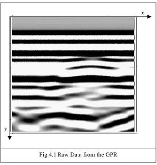
The raw data from the GPR is illustrated in Fig 4.1. The x-axis represents the motion of the

GPR along the surface and the y-axis (increasing downwards) indicates time.

y

x

Fig 4.1 Raw Data from the GPR

From this initial GPR image the reconstruction or object extraction process constitutes two

main steps.

a) Background Removal.

b) Data Migration.

i) Correlation of the transmitted signal

(35)

After these two steps, post-processing includes steps such as thresholding and object

extraction.

4.1 BACKGROUND REMOVAL BASED ON “SUBTRACT

TRANSMITTED PULSE”

The received data contains the “direct wave”, the reflected waves and external noise. The

instrument is designed such that the receiver continues to listen even as the transmitter sends

out the pulses. This effect is primarily due to the close proximity of the transmitting and

receiving antennae. As a result, the receiver picks up the transmitted wave and superimposes

it on the reflected signals. Since the transmitted signal is strong due to the close proximity of

the antenna to the receiver, it is very bright and thus it is difficult to identify gradients in the

image. The transmitted wave must be removed. There are two methods that were used to do

this, a) using a sample transmitted pulse and b) subtracting the mean trace.

In the “Subtract Transmitted Pulse” method, a sample pulse is subtracted from the entire

image. This sample pulse is extracted from GPR data recorded in an empty environment. The

running time of this algorithm is θ(n), where n is the number of pixels. Though quick, this

algorithm does not consider the dynamic nature of the working environment, and hence at

times the sample input wave does not exactly coincide with the actual wave used in practice.

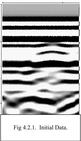
This method leaves heavy traces of the input signal that are considered as anomalies by the

migration algorithm. A sample input image and its filtered output are shown in Fig 4.2.1 and

(36)

Fig 4.2.2. Filtered Result from the “Subtract Transmitted Pulse” method. Fig 4.2.1. Initial Data.

This technique only considers the transmitted signal and does not eliminate any external

noise.

4.2 BACKGROUND REMOVAL BASED ON “SUBTRACT MEAN

TRACE”

In this method we define a window of around 30 – 40 pixels and subtract from all the pixels

in this window the mean of the pixels in it. The window is moved along and the procedure is

repeated until the entire image is covered, as given in Equation 4.1.

∑

= − = + − = 2 2 ) , ( 1 ) , ( ) , ( m i m i y i x f m y x f y x

g 4.1

(37)

Fig 4.3.2. Filtered Result using the “Subtract Mean

Trace” method. Fig 4.3.1. Initial Data.

This method does not require any prior knowledge of the GPR signal. The running time of

this algorithm is the window size multiplied by the previous method. As a result, selection of

a large window requires more processing time, which is critical in real time applications. A

sample input image and its filtered output are shown in Fig 4.4.1 and Fig 4.4.2.

Running time (Subtract Mean Trace) = m * Running time (Subtract transmitted pulse)

(38)

Sample filtered images for window sizes 30 and 200 pixels are shown in Fig 4.4.1 and Fig

4.4.2 respectively. After experimentation, the optimum window size was found to be between

(39)

5. DATA MIGRATION

5.1 CORRELATION OF THE TRANSMITTED SIGNAL

5.1.1 Signal Description and Simulation

The transmitted pulse (direct wave) of the GPR is not an impulse. It rather resembles a

Gaussian modulated sine wave (as shown in Fig 5.1). As a result, the reflections returning

from different objects are varying magnitudes of this wave.

Amplitude

Fig 5.1 Transmitted signal modeled by a Gaussian modulated sine wave

(Signal S) T

i m

e

As the observed image g is the result of a convolution between the actual image f and the

(40)

∑

− × =

i

i s i y x f y

x

g( , ) ( , ) ( )

where i denotes the number of elements in the input signal s. The x-axis denotes the position

of the GPR and the y-axis denotes time.

In order to obtain an optimum algorithm for the reconstruction, we initially simulate a GPR

image in order to have a better control over the algorithm development. Once an algorithm is

designed, the method is extended to actual data from the GPR.

The simulation of a disc placed under the ground surface is shown in Fig 5.2. The horizontal

axis represents the line along which the GPR moves and the vertical axis denotes the depth of

the object. Only the upper half of the disc is considered.

Single Column X

(41)

When the transmitted wave (S) as modeled in Fig 5.1 is reflected in part from the circular

disk as shown in Fig 5.2, the signals received by the GPR appear as shown in Fig 5.3. Each

part of the disk reflects a certain amplitude of the direct wave.

Single Column X

Fig 5.3 Received image from the GPR (Simulated).

5.1.2 Linear Correlation Coefficient (LCC)

The linear correlation coefficient (r) is a quantity that determines the relationship between

two functions. Its value ranges from –1 to +1. +1 indicates a direct relationship between the

two functions, 0 indicates no relationship and –1 indicates an inverse relationship. The square

of this coefficient, r2, also known as the coefficient of determination, determines the variance

(42)

∑

= = = − − − − ≡ n i i n i i n i i i xy y y x x y y x x r 1 2 1 2 1 ) ( ) ( ) )( ( 5.1

where x and y are the two functions with n values each.

x is the mean value of x defined as

∑

= n i i x n 1 1

and y is the mean value of y defined as

∑

= n i i y n 1 1 .

In order to reverse the correlation caused by the transmitted wave, we isolate the returned

image (Fig 5.3) into individual columns. This can be done assuming that the result of the

correlation in a single column (one particular position of the GPR) is independent of the data

present in the remainder of the image. Hence we have now reduced the problem to a

reconstruction in one dimension.

If we consider the column corresponding to the center of the circular disc (Column X) in Fig

(43)

Amplitude

Fig 5.4 Column representation of the center of the disk. (Column X) T

i m

e

The impulse in the above figure corresponds to the bright spot on the disc, which was

roughly at a depth (position) of 300 pixels. In order to avoid the unreasonable case of a

homogenous background, we added Gaussian noise with a standard deviation of 0.1 to all the

remaining pixels that comprised the soil beneath the surface. The result of the correlation

(44)

Amplitude

Fig 5.5 Result of the Correlation. (Column Y)

T i m

e

In order to invert the correlation we use the linear correlation coefficient (r) from Eq. 5.1.

The pseudocode for the calculation of r is shown below.

for j = 51 to (1000 – 51) do (no of elements in a single column)

R[j] = 0.0;

for n = -50 to +50 do (101 elements in the input signal S)

R[j] += Y[j + n] x S[50 + n].

As the input signal S contains 101 elements, n in this equation is set to 101. To calculate r at

a particular pixel (i) from Column Y, we need to select 101 elements including pixel i. We do

this by selecting i as the 51st_{element and completing the array of 101 by taking 50}

continuous elements from either side of i. This process has to be repeated 1000 times to

(45)

101 elements, there are 50 pixels at the beginning and 50 pixels at the end of Column Y that

do not have a value.

The linear correlation coefficient for the elements in Column Y with the input signal S is

shown below.

SY r

Amplitude

T i m

e

SY r

Fig 5.6 Reconstructed image - Linear Correlation Coefficient (Column

F).

As negative values of r indicates inverse relationships, we ignore all negative values of r.

Our simulation assumes that there can only be one object in a particular column, i.e. there

cannot be two objects one below the other. Hence there can only be one bright spot in one

column. In the above image (Column F), this maximum value (1.0 in this case, which

(46)

where we had the bright spot originally (Column X). Consequentially, the maximum value of

each column should correspond to an object. This however is not the case, as only the

maximum value of each column that is greater than a particular threshold value represents an

object.

In practice it was observed that even though the filtered images of actual GPR data (Fig 4.4)

do not have perfect discs or features as shown in Fig 5.2, but rather hyperbolic

representations of these objects, the correlation of the input signal results in an image which

contains columns that are independent of each other. Hence the linear correlation coefficient

method can be applied successfully without any modifications.

In order to implement the above algorithm to real data, an iron pipe 25 inches in length and 7

inches in diameter was placed 15 inches deep in a sandbox. The pipe was kept perpendicular

to the line of motion of the GPR. The soil used in this experiment was dry sand.

Fig 5.8 Result of the LCC technique applied to Fig 5.7.

(47)

Fig 5.7 shows the filtered result of the measurement. When the LCC technique is applied to

this image, the result after thresholding is shown in Fig 5.8. The input signal S used in this

case is the actual wave of the GPR, which is shown in Fig 1.2. The original image comprised

of 923 columns and 1024 rows. The algorithm took approximately18 seconds to run on a

Pentium 4 2000. Hence, as the reconstruction resembles a hyperbola with a dark background,

it can be reduced to its original form using the technique presented in Section 5.2.

5.2 ANTENNA SIGNAL SPREAD

In order to reconstruct the hyperbolae caused due to the signal spread of the GPR, we

construct an objective function as explained in Chapter 3 and attempt to optimize it such that

it converges to one particular solution based on certain parameters of the original image that

we shall define. As explained the objective function comprises of two terms, the noise term

and the prior term. The parameters of the original image are incorporated in the prior term.

5.2.1 Incorporating the Prior and Noise Terms

A model was created to simulate the signal spread of the antenna. A circular disc was used as

the object of choice.

Noise term

Originally the noise term Hn (from Eq 3.10) looks like

=

∑

i − i n

g f H

2

) ' (

(48)

This equation was differentiated to be included in the minimization of the objective function.

It then takes the form (from Eq. 3.13)

1₂[( )_i _i] _rev.

i

n _f _h _g _h

f H

⊗ − ⊗ =

∂ ∂

σ 5.3

where h represents the kernel to be applied and hrevrepresents the reverse of this kernel.

We have to construct the kernel (h) that models the antenna spread. The model of the signal

spread is shown in Fig 5.9. From experimental observations we have concluded that the

spread angle of the GPR is modeled (as best described by literature and experimentation) to

be around 45 degrees. Also, the wave front is assumed to be circular. We model the signal

spread in two dimensions and hence the wave appears as a sector subtended at an angle of 45

degrees on either side of the normal to the GPR. Effectively we get a sector with a radius

corresponding to the depth and a total angle of 90 degrees. The kernel (h) is effectively the

outer arc of this sector, the arc length of which is calculated from the parameters discussed

above.

L

t

Fig 5.9 GPR Signal Spread with the sensor at xo. GPR at (xo,0)

x

(49)

The position of the GPR is given by (xo,0). y signifies depth and increases in the downward

direction.

In the 2-dimensional – x,y - case we model the signal generation process as

∑

+

−

= θ

θ

) , ( ) , ( )

,

(x t f x y h x x t

g _o _o

f is the original image, g is the measured image and h is the kernel The GPR is located at

(xo,0) and remains fixed for one measurement. t denotes time and θ is the angle of spread.

The form of h depends on t, as h is the curve corresponding to a particular value of t. h is

time-variant. Depth (y) and time (t) are interrelated. We measure both of them in the same

units, pixels. For the arc L, all the points lying on the arc are equidistant from the source in

terms of time, but not in terms of depth. Hence during our measurements we need to convert

time into depth. For a fixed position of the GPR (xo,0), the x and y coordinates of the

different points on the arc are given in terms of time t as

. cos

0 t θ

x x= +

. sinθ t y=

where θ is the angle of the signal spread.

The simulation moves the signal source from one end of the image to another. At each

position of the signal source, for different times (pixels), we calculate the arc length and

apply that as a kernel to the image at that pixel (same as equation 5.4). We store the result for

each pixel in an array (another image). This process is repeated for the next position of the

(50)

The signal is considered to be at its strongest down the center of the cone and attenuates

gradually away from the center. The signal of the GPR attenuates heavily as it propagates

deeper into the surface. The simulation incorporates this using an attenuation parameter that

moderately models that of the GPR. Experimentation with objects placed at different depths

the yielded the following results.

Original Strength of the signal / Response from an object 100 pixels deep = 113.

Original Strength of the signal / Response from an object 500 pixels deep = 527.

These responses however were from objects placed in dry sand. For wet clay the signal

strengths drop down by a further one third due to the refractive index of wet clay. Since the

medium of observation for all the experiments was chosen as dry sand we choose an

approximate attenuation parameter of 1/t where, where t≠ 0, corresponds to the object depth

in pixels.

In order to reverse of the kernel (outer kernel in Eq 5.3), the same process is repeated with an

inverted kernel. The kernel is inverted about the y-axis, i.e. we take a mirror image of the arc

that we used before and apply it to the result of the above operation.

Prior term

In Eq 3.11 we defined the prior term Hpas

.

2

1 2

2

2 ) (

∑

− ⊗

− =

i

r f

p

i e

H τ

τ

π 5.5

(51)

[( ) ] .. 2 2 1 2 2 2 ) ( 3 rev r f i i p r e r f f H i ⊗ ⋅ ⊗ = ∂ ∂ − ⊗ τ τ

π 5.6

In order to incorporate a prior term we need to possess some knowledge of the original image

before it was distorted. In this case we know that the original image comprises a bright disc

kept in a dark background. In case of actual GPR data, the filtered and reconstructed image

(from section 5.1) is supposed to have bright curves corresponding to the edges of the

different objects against a dark background. Hence the prior term we selected smoothes the

image (in order to eliminate noise) while preserving the strong edges (which correspond to

the outline of the disc). We model the prior term as piecewise linear, which means that we

assume that the model consists of segments that are planar (considering that the intensity as a

function of x and y is a plane). This model has been used effectively in [3], [31]. A planar

form results if one chooses to minimize the effects of the second derivatives. Thus following

[3] [31] we define the prior with the help of three kernels.

          − = ∆ 0 0 0 1 2 1 0 0 0 6 1

xx ,

          − = ∆ 0 1 0 0 2 0 0 1 0 6 1

yy ,

          − − = ∆ 25 . 0 0 25 . 0 0 0 0 25 . 0 0 25 . 0 2 xy xx

∆ is a kernel which when applied to image f approximates ₂ .

2

x f

∂ ∂

Similarly ∆_yy

approximates ₂

2

y f

∂ ∂

and ∆_xy approximates .

2

xy f

∂ ∂

In order to identify edges about a particular pixel we place the kernel over it. As a result the

(52)

neighbors are multiplied by the respective values in the matrix. The magnitude of this result

is proportional to the edge strength of that pixel.

As shown in Eq 3.14 and Eq 3.15, after the prior term is differentiated, the result of the first

convolution (with r) is further convolved with the reverse of the kernel (rrev) used for the first

convolution. Before we apply the reverse kernel we take the results of the three kernels

applied to the image (f⊗r) and use them in the exponential in equation 5.5. These values are

stored separately. Next, we perform the second convolution (with rrev) using the three results.

The kernels for rrev are shown below. Notice that due to their symmetry only the form of ∆_xy

changes.           − = ∆ 0 0 0 1 2 1 0 0 0 6 1

xx ,

          − = ∆ 0 1 0 0 2 0 0 1 0 6 1

yy ,

          − − = ∆ 25 . 0 0 25 . 0 0 0 0 25 . 0 0 25 . 0 2 xy

These values are then used to create the prior term that is added with the noise term to

give us the derivative of the objective (H) function.

5.2.2 Gradient Descent and the MFA Algorithm

The gradient descent equation is given as

1 , l k k l k l f H f f ∂ ∂ − = + _α 5.7

where H is the objective function (in our case either Hn or Hp), k is the iteration number, fl is

one element of the vector representation of the image f and α , the “step size”, is a constant

(53)

The image obtained after the filtering and the reconstruction from section 5.1 is used as the

initial estimate in equation 5.7. This image is used in the noise and the prior terms to get the

difference f H

∂ ∂

. This difference is multiplied by α and subtracted from the initial estimate.

This becomes the input image for the next iteration of the gradient descent and so on till we

arrive at an estimate that does not produce a sizeable change in the term f H

∂ ∂

.

MFA is incorporated by setting the τ in the prior term to a very large value initially. This

makes the prior term zero to begin with and as the algorithm progresses τ is decreased by a

factor of 0.99 at each iteration to make the prior term more and more comparable in

magnitude to the noise term. As explained in section 3.3 this approach tends to avoid most

local minima and converges at solutions that are nearly global.

Results

Fig 5.10 shows the simulated representation of a disk placed beneath the soil surface. The

horizontal axis represents the line along which the GPR moves (assumed from left to right)

and the vertical axis denotes the depth of the object. As most of the waves from the

transmitter bounce off the top of the object, only the upper half of the disk is used in the

(54)

Fig 5.10 Simulated image of the upper half of a disk placed under a soil surface.

The result of the convolution from can be seen in Fig 5.11. The disk now looks like a

hyperbola, which has its center coinciding with the center of the disk. As explained, this

occurs due to the breadth of the signal spread of the GPR. The signals get attenuated as the

distance traveled increases and hence pixels at a greater depth are relatively dimmer than the

ones higher up.

Figure 5.11. Hyperbolic Representation (convolution) of the disk caused by the signal of the GPR.

The MFA algorithm is applied to the image in Fig 5.11. After using the measured image (Fig

5.11) as the initial estimate for the MFA algorithm, the algorithm converges to the image in

(55)

Figure 5.13. What the complete disk would have looked like Figure 5.12. Reconstruction of the disk

using the MFA algorithm.

It can be seen that most only the area corresponding to the top of the disk is bright. Fig 5.13

illustrates what the complete reconstruction would have looked like. A possible explanation

as to why only part of the disk is visible in Fig 5.12 is that only the top of the disk remains

intact after the initial convolution (Fig 5.11). The hyperbolae resulting from the surface of

the disk mixes up with the area corresponding to the remaining portions of the disk, which

get obscured and appear as part of the spread caused by the surface pixels. The reconstruction

is unable to differentiate between the original portion and the spread. This causes the

algorithm to eliminate the original area along with most of the spread during the

reconstruction. As a result only the original part of the disk that wasn’t corrupted by the

(56)

The energy curve for successive iterations of the MFA algorithm is shown in Fig 5.14. The

energy term indicates the difference in images in consecutive iterations, also considered as an

error. The algorithm converges to a solution when this error is minimized. In the case above,

this happens at the 92nd iteration after which the algorithm moves away from the solution.

Energy vs Iterations

0 5 10 15 20 25 30 35 40

0 10 20 30 40 50 60 70 80 90 100 110 120 130 140 150

Iterations

Energy

Figure 5.14. Energy Curve of the MFA algorithm.

Minimum at the 92nd

iteration.

Fig 5.15 shows the effect of noise on the reconstruction. The error is close to 0 when minimal

(57)

increases steeply for lower SNR values. Error values greater than 75 units create a difficulty

in object detection.

Signal to Noise vs Error

0 50 100 150 200 250 300

1.33 2 2.5 3.33 4 5 6.66 10 16.66 33.33 100 No

Error Signal to Noise Ratio

Error

(58)

6. CONCLUSION

The process of reconstruction of images from the GPR is broken down into various parts due

to the complex nature of the data recording process of the RAMAC GPR. Many papers have

presented techniques to reconstruct part of the data, but very few have addressed the

reconstruction in its entirety.

Due to the proximity of the antenna to the receiver, the instrument records and superimposes

the transmitted wave over the received signals. The process of utility detection is complicated

due to the strength of the transmitted signal. We propose two methods to remove the

transmitted signal. The “Subtract Transmitted Pulse” method subtracts a sample-transmitted

pulse from the entire image. This algorithm runs fast but tends to leave behind heavy traces

of the input signal. The “Subtract Mean Trace” method takes the average of all pixels within

a horizontal window and subtracts this average from all the elements in that window. The

running time of this algorithm is slower as compared to the previous technique but it removes

the transmitted wave almost completely. The ideal window size was found to be between 30

and 40 pixels.

As a single pulse of the GPR is not an impulse but rather a wave that looks similar to a

Gaussian Modulated Sine Wave (GMSW), the reflections from the utilities are magnitudes of

this wave. Hence any object in the image appears as a collection of black and white bands.

We used a technique based on the linear correlation coefficient (LCC) to reconstruct the

pulses. However, we assume that there would not be a case where two objects would be

Reconstruction of Ground Penetrating Radar Images using techniques based on Optimization.

R

O

G

P

R

I

U

T

B

O

O

TABLE OF CONTENTS

1. PROBLEM

DESCRIPTION

1.1 INTRODUCTION

1.2 WHAT IS A GPR?

1.3 MATERIAL

CONDUCTIVITY

1.4 DATA

MIGRATION

∑

∑

2. LITERATURE

REVIEW

2.1 GPR ANTENNA CHARACTERIZATION

2.2 CATEGORIZATION OF OBJECT RECONSTRUCTION

TECHNIQUES

∑

∫

2.3 GPRS USED IN MINE DETECTION

2.4 RECONSTRUCTIONS BASED ON OPTIMIZATION

2.5 ALGORITHMS FOR THE INVERSION OF THE TRANSMITTED

WAVE

2.6 MIGRATION

ALGORITHMS

3. OPTIMIZATION

ALGORITHM

3.1 CONSTRUCTING THE OBJECTIVE FUNCTION

∏

∏

∑

∑

∑

∑

∑

3.2 GRADIENT

DESCENT

3.3 MEAN FIELD ANNEALING

4. PRIMARY PROCESSING OF THE RECEIVED GPR

SIGNAL

4.1 BACKGROUND REMOVAL BASED ON “SUBTRACT

TRANSMITTED PULSE”

4.2 BACKGROUND REMOVAL BASED ON “SUBTRACT MEAN

TRACE”

∑

5. DATA MIGRATION

5.1 CORRELATION OF THE TRANSMITTED SIGNAL

∑

∑

∑

∑

∑

∑

5.2 ANTENNA SIGNAL SPREAD

∑

∑

∑

6. CONCLUSION