Relationship between Microstructure and Mechanical Properties in Bi2Sr2CaCu2Ox Round Wires Using Peridynamic Simulation.

LE, QUANG VAN. Relationship between Microstructure and Mechanical Properties in Bi2Sr2CaCu2Ox Round Wires Using Peridynamic Simulation. (Under the direction of Justin Schwartz).

© Copyright 2014 by Quang Van Le All Rights Reserved

by Quang Van Le

A dissertation submitted to the Graduate Faculty of the North Carolina State University

in partial fulfillment of the requirements for the degree of

Doctor of Philosophy

Materials Science & Engineering

Raleigh, North Carolina 2014

APPROVED BY:

________________________________ __________________________________ Justin Schwarz Douglas Irving

Committee Chair

BIOGRAPHY

Quang Le is drawn to science because to him, it is just another way of saying “magic”. Quang received his M.S. from Florida State University in 2009 and is currently a Ph.D. student at North Carolina State University. He is experienced in both experimental and theoretical studies of electro-mechanical properties. He is set to graduate in 2014 and hopes to continue conducting research after graduation.

ACKNOWLEDGEMENTS 

I would like to express my gratitude to these persons for all their helps. Without them, I would not be able to be where I am today 

‐ My advisor Justin Schwartz for his support and guidance throughout my long study.  ‐ Former mentor Abdallah Mbaruku for his teaching and helping on my very first steps

of being a graduate student. 

‐ Ronald Scattergood, Douglas Irving, and Mohammed Zikry for serving on my committee. 

‐ Wan Kan Chan for helpful discussions and guidance.  ‐ My colleagues for collaboration and being great friends. 

‐ And last but not least, my family for their eternal support and encouragement.    

TABLE OF CONTENTS

LIST OF FIGURES ... vi 

1.  INTRODUCTION ... 1 

1.1. Superconductors ... 1

1.2. High Temperature Superconductors ... 2

1.3. Bi2212 Round Wires ... 4

1.4. Peridynamic Theory ... 22

1.4.1. Peridynamics as a Non-local Theory ... 22

1.4.2. Relations between Classical Mechanics and Peridynamics ... 35

1.4.3. Peridynamic Applications ... 40

2.  2D STATE BASED PERIDYNAMICS ... 50 

2.1. Introduction ... 50

2.2. Peridynamic Model for 2D Plane Stress... 51

2.3. Peridynamic Model for 2D Plane Strain... 57

2.4. Simulation Approach ... 59

2.4.1. Finding the Peridynamic Steady-State Solution... 59

2.4.2. Modifying the Node Interaction Volume ... 64

2.5. Verification with FEM Analysis... 65

2.5.1. Convergence to Continuum Peridynamics ... 67

2.5.2. Convergence to Classical Mechanics ... 70

2.6. Peridynamics Stress at the Sharp Corners ... 74

3.1. Scanning Electron Microscopy Image Analysis ... 78

3.2. Peridynamics System Construction ... 81

3.3. Peridynamic Simulation Method ... 85

3.4. Simulation Results ... 86

3.4.1. Samples with no defect ... 87

3.4.2. Samples with a single natural defect from a SEM image ... 91

3.4.3. Samples with a multiple natural defects from a SEM image ... 93

3.4.4. Samples with rectangle artificial defects of different vertical lengths ... 95

3.4.5. Samples with rectangle artificial defects of different horizontal widths ... 99

3.4.6. Samples with 45degree slanted artificial defects of different widths ... 102

3.4.7. Samples with circular defects of different diameters ... 105

3.4.8. Samples with artificial rectangle voids inside a Bi2212 filament ... 109

3.4.9. Sample with artificial voids around a Bi2212 filament ... 111

3.4.10. Simulation of stress concentration due to thermal cooling ... 112

4.  CONCLUSION AND SUGGESTED FUTURE WORK ... 115 

REFERENCES ... 120 

LIST OF FIGURES

Figure 1.10. Relationship between 4.2 K, self-field Je, bridge size and bridge area percentage (of the non-Ag area) with bridges size, (a) 0–1 μm; (b) 1–2 μm; (c) 2–3 μm and (d) 3–4 μm

[4]. ... 15

Figure 1.11. Dependence of critical current on compressive and tensile strains in Bi2212 in modified descriptive strain model [10]. ... 17

Figure 1.12. Original and simulated microstructures using fractal analysis [15]. ... 21

Figure 1.13. Steady-state von-Mises stress distribution with fixed load of 60 N/m to simulated microstructure [15]. ... 22

Figure 1.14. Interaction forces between 2 points in an ordinary peridynamic system. ... 24

Figure 1.15. Undeformed and deformed peridynamic bonds. ... 26

Figure 1.16. Dependence of different influence functions on bond vector. ... 28

Figure 1.17. Crack propagation speed with three different horizon sizes [38]. ... 33

Figure 1.18. Dispersion relations for various values of p. (a) with influence function in equation (1.18). (b) with influence function in equation (1.19) [23]. ... 34

Figure 1.19. Impact of a hard sphere on a disc of brittle material at 5x10-5s after impact. (a) p = 0. (b) p = 5. (c) p = 10 [23]. ... 35

Figure 1.20. Force acting on a surface in classical mechanics. ... 36

Figure 1.21. Interpretation of the force flux at x across a plane with unit normal n [41]. ... 39

Figure 1.22. Damaged maps for tests of crack path instability and branching, with sudden loads on top and bottom. (a) 12 MPa load, t = 46 μs. (b) 27 MPa load, t = 38 μs [42]. ... 41

1. INTRODUCTION

1.1. Superconductors

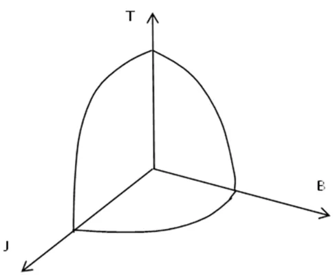
Superconductors are materials that can carry an electrical current without generating heat. This is a desired property for applications where reducing energy waste or high current density is critical; since a resistive conductor with a high current will generate much heat and may damage the system. Superconductors show promises in applications using high field magnets such as maglev trains, magnetic resonance imaging, nuclear magnetic resonance, or in power transfer and storage applications. Other applications include digital circuits and sensitive magnetic sensors.

Figure 1.1. Superconductivity surface: superconductivity exists only when temperature, magnetic field, and current density all smaller than critical values.

After the discovery in mercury, tin, and lead, superconductivity was discovered in most other elements as well. Most pure elements (except vanadium, technetium and niobium) have type 1 superconductivity, in these superconductors the Meissner effect is an all or nothing phenomenon. If the magnetic field is less than critical value, no magnetic flux penetrates the material. But if the magnetic field is higher than that critical value, superconductivity is lost totally and the magnetic field penetrates the material completely.

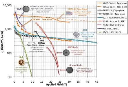
1.2. High Temperature Superconductors

Figure 1.2. Engineering critical current density versus magnetic field for low temperature superconductor wires, high temperature superconductor wires and tapes

and MgB2 wires [1].

1.3. Bi2212 Round Wires

conductor reliability as a function of critical current. The statistical approach is needed is because even individual samples of the same heat treatment batch, under the same mechanical loading condition, usually have different critical currents. On Figure 1.3 the

reliability at a certain value of Ic on the graph is the probability a sample will have the current of at least that Ic value or higher. By definition, this probability is equal to 1 at zero critical current because every sample has a critical current of at least zero.

The reliability does not necessarily decrease immediately as Ic increases, in fact for samples under no mechanical loading (strain equal to zero), reliability stay constantly equal to one until Ic reaches the critical value γ = 579A. This means at no load condition, it is certain that every sample has critical current of at least 579A or higher. Value of γ however decreases markedly with loading strain: when strain increases from 0% to 0.25%, γ decreases from 579A to 448.1A. When strain increases to 0.40%, γ approaches 0A. This means at strain of 0.40%, there is no certainty that a sample will carry a non-zero superconducting current. From this statistical analysis, one can see that the current carrying performance depends not only on the loading condition but also on individual samples. One question remains: how do samples have such large variation in performance even when they undergo the same manufacturing processes?  

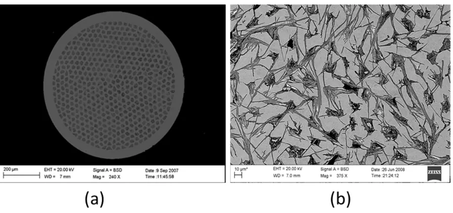
One possible explanation is the variation in the electrical performance is caused by the variation in the micro-structure of the superconducting wire, which in turn is highly sensitive to heat treatment parameters. Powder-in-tube method is used in the manufacturing of the Bi2212 wires, in which Bi2212 powder is filled in silver tubes, and then the tubes are drawn to create the untreated or “green” wires. The green wires become superconducting after they have gone through a heat treatment process to create connected, solid Bi2212 filaments from the initial powder. As Figure 1.4(a) shows, there are hundreds of untreated Bi2212 filaments inside a green wire and initially, they are all separated from each other. However, Figure

1.4(b) shows after a heat treatment, there are voids, multiple phases and intergrowth between

Figure 1.4. Cross-sectional scanning electron microscopy images of Bi2112 round wires: (a) Before heat treatment, and (b) After heat treatment.

Figure 1.5. Temperature–time schematics (not to scale) of the heat treatment profiles for (a) partial-melt processing, (b) split-melt processing, and (c) saw-tooth processing

[3] .

It has been found the split melt process results in 40% increase in critical current in Bi2212

round wires, compared the to the partial melt process [6]. While study [3] shows that a

However, all heat treatment processes are often not 100% effective. As mentioned above, other than the Bi2212 superconducting phase and silver, there are also remaining non-superconducting phases and bubbles/voids. Limiting the amount of these phases is often the underlying mechanism for improving the material’s performance.

Figure 1.6. (a) Tomographic image of a heat treated wire, dark gray areas are bubbles. (b) Scanning electron microscopy image of a cut-out Bi2212 filament, showing the

hollow core inside it [5].

while the wire with iso-static pressing achieves 3661 A/mm2. The reason why the cold pressing results in such improvement is it densifies the (untreated) wires, resulting in lower porosity or the volume fraction of the bubbles in the wires. Also, in the study, SEM image analysis of the quenched samples shows a change in shape and size of the bubbles. The wires without cold pressing have elongated bubbles with length about 2-3 times their diameters, while the wires undergoing the cold pressing have smaller and more rounded bubbles.

Similar to bubbles, non-superconducting phases also limit or block the current flow inside the Bi2212 filaments. Thus by reducing their volume fractions, one could also improve the performance of the wires. One of the methods of doing so is the saw-tooth heat treatment process [3]. In the process, by the multiple heating and cooling cycles, more nucleation sites for growing the superconducting phase Bi2212 are formed compared to just one cycle as in the split-melt process. This results in a higher percentage of the superconducting phase Bi2212, and conversely, lower percentages of other non-superconducting phases. Figure

1.7(a) shows an example of a filament where a significant fraction is the

non-superconducting phase Bi2201 (light gray) instead of the desired non-superconducting phase

Bi2212 (dark gray). Such filament would not conduct current well. While Figure 1.7(b)

shows a dense filament comprised of mostly the Bi2212 phase. It is found in [3] that more

Figure 1.7. Cross-sectional SEM images of (a) filament with significant amount of Bi22012 phase and (b) filament consisting mostly Bi2212 phase [3].

Another important microstructure feature in Bi2212 round wires is the intergrowths between

the Bi2212 filaments. In the study [4], it is found that by varying the split and the return

temperatures of the split-melt process, there’s a significant change in microstructure of the

wires and consequently, the electrical performance. Specifically, the amount of intergrowths

between the superconducting filaments is highly dependent on both the split and the return

temperatures. Figure 1.8 (a) shows an example cross-sectional SEM image of the wire, while

Figure 1.8(b) shows the transformed image of Figure 1.8(a) by analyzing and marking the

superconducting areas different colors by different thicknesses. The red color corresponds to

areas with half-width from 0 to 1 micron, yellow: 1 to 2 microns, green: 2 to 3 microns, blue:

Figure 1.8. (a) Original cross-sectional SEM image analysis of Bi2212 wire showing intergrowths between the filaments. (b) Image analysis: bridges with different widths

are marked with different colors from red to blue.

By analysis of SEM images of multiple wires then matching the results with heat treatment

profiles, relationships between bridges growth and heat treatment temperatures are

established [4]. Figure 1.9(a) shows the correlation between the split temperature and the

volume percentage of bridges/intergrowths. Similarly, Figure 1.9(b) shows the correlation

between return temperature and the bridges volume percentage. In the range of the

temperatures investigated, there is a positive relation between the temperatures and the

Figure 1.9. (a) Relationship between split temperature and bridge size and bridge area percentage. (b) Relationship between return temperature and bridge size and bridge

area percentage [4].

Also, matching the image analysis results with data on critical current densities of the wires

shows the strong correlation between bridge percentage and electrical performance. More

specifically, Figure 1.10 shows that when the bridges are categorized by sizes, the larger

bridges (Figures 1.10(c) and 1.10(d)) have a strong positive correlation with effective critical

Figure 1.10. Relationship between 4.2 K, self-field Je, bridge size and bridge area percentage (of the non-Ag area) with bridges size, (a) 0–1 μm; (b) 1–2 μm; (c) 2–3 μm

and (d) 3–4 μm [4].

One possible explanation for this behavior is the intergrowths enhance the connectivity of the

previously, there are bubbles and non-superconducting phases inside Bii2212 filaments. They

can severely limit the current running through them or even block the current completely.

When this happens in a filament, the intergrowths allow other pathways for the current to

flow from the blocked filament to other ones. In other words, the relationship between the

filaments and the intergrowths is similar to a system of highways and detours. When one

highway gets congested, traffic can redirect to detours to get into other highways. This

enhanced connectivity results in higher electrical performance. The reason why thicker

bridges have more influence than thinner bridges on performance could be simply because

the thicker bridges can bypass a higher electric current from filament to filament because of

their bigger sizes. Also, another possible explanation is thicker bridges tend to be made of

single grain, while thinner bridges can be formed from joined grains with different

orientations [8]. Grain boundaries (especially high angle ones) are barriers to

superconducting currents. Thus qualitatively the single grain bridges can carry currents better

than the multi-grain bridges.

than a critical value and irreversible/degrading behavior when the strain is higher than the critical value.

Experimentally, it has been found that this threshold strain value varies from wire to wire, with the average value about 0.31% in tension. From zero to 0.31% applied tensile strain, the critical current slightly decreases when the applied strain increases. In the study, it is considered that in this region, the Bi2212 phase is actually in the compressive state. The reason is due to differences in thermal expansion coefficients, when the Bi2212 wire is cooled from room temperature to cryogenic temperature where experiments are taken, the B-i2212 phase will be in compression stress/strain state, while silver is in expansion state. So the externally applied strain in this region only alleviates the internal compression already present in the B-i2212 phase, and around the critical applied strain 0.31% is where the externally applied strain neutralizes the internal strain in Bi2212. The irreversible degradation of critical current at strains larger than 0.31% is stipulated as the result of the cracking in Bi2212 filaments in tension.

support from the silver matrix. Although the descriptive models are reasonable, there need more understandings as well as quantitative experiments to confirm the suggestions of the models. However, due to the micro-scale of the features in Bi2212 wires, experimental approaches would face significant difficulties to be conducted at such as small scale.

So far, it has been found that that bubbles, non-superconducting phases, and filament shapes and inter-filamentary bridges all play important roles in the electrical performance for the Bi2212 round wires. But how do they influence the mechanical behavior? For example, do wires with bubbles have lower strength than wires without them, and how much lower? Or how do the spatial arrangements of different phases affect the relationship between local strain and the macroscopic strain? The micrometer scale of these features in Bi2212 round wires make it difficult for experimental approaches to correlate a specific microstructure feature to the material’s mechanical behavior, since each wire can contain multiple features. Since mechanical experiments on these wires are usually implemented on macroscopic scale, it is challenging to correlate some specific microstructure features and the macroscopic properties.

investigate the system’s behavior. The reason is classical mechanics rely on partial differential equations to establish the constitutive stress-strain relationship in the material. Classical approaches using finite element method usually requires rounding off the geometry at those sharp corners.

In order to eliminate those rough edges/sharp corners, in [15] a fractal analysis is used to re-generate the microstructure of the Bi2212 wires. In the study, a longitudinal SEM image of Bi2212 filament is used to analyze the irregular shape of the boundary between the Bi2212 filament and the silver matrix. A fractal dimension number is assigned to this boundary line. Then using computer simulation, fractal curves of the same fractal dimension number (as the original line) are generated. Figure 1.12(b) shows a simulated microstructure in which, two fractal curves are used for generating the Bi2212/silver interface. The computer generated fractal curves in Figure 1.12(b) have the same fractal dimension of the real silver/Bi2212

boundary curves obtained from the Figure 1.12(a). The computer generated fractal curves

Figure 1.12. Original and simulated microstructures using fractal analysis [15].

Figure 1.13 shows the von-Mises stress distribution in the simulated microstructure. Stress

Figure 1.13. Steady-state von-Mises stress distribution with fixed load of 60 N/m to simulated microstructure [15].

1.4.Peridynamic Theory

1.4.1. Peridynamics as a Non-local Theory

undefined there. Thus one needs to redefine the body and its boundary so the cracks are on the boundary [16]. Also, at phase boundary where coordinates are defined and continuous, their spatial derivatives are not continuous - there is a jump at the interface. This also requires classical mechanics to define the phase boundary and its corresponding boundary conditions. For a composite material with complex phase structure, this could lead to complex boundary problems. So far, finite element method (FEM) is the most commonly used to simulate mechanical behaviors of a material or system. Since FEM is based on partial

differential equations, stress and strain singularities at sharp corners create undefined

derivatives at these regions, resulting in convergence problems. Especially in materials with

complex phase arrangements where there are many “sharp corners” at the phase boundaries

or voids, FEM faces significant difficulties. Partial differential equations are also limited with

respect to systems with discontinuities such as cracks. Additional modeling techniques, such

as adaptive meshing, are required to model the growth of an existing crack.

interactions between discrete points, in peridynamic theory material points are continuous, like in classical mechanics. It is just that in practice of computer modeling and simulation, the continuum peridynamic body is approximated by a discrete set of peridynamic nodes. Finally, the difference between peridynamics and classical mechanics is peridynamics uses integral equations instead of partial derivative equations for its formulas, and the force interactions happen over a finite distance instead of contact/ local forces.

Figure 1.14 shows the schematic of interaction between 2 points in peridynamic theory. In

the figure, each peridynamic point interacts with all other points around it within a cut off distance δ called the horizon.

In peridynamics, the motion of a point depends on forces other points acting on it:

¨ , , , d , (1.1)

where is the mass density at reference point x (kg/m3). u is the displacement of point x at time t. H is the neighborhood region of point x containing all points that interact with it. The region of H depends on the specific peridynamic model, usually it is defined as a region around the point x within the cut off distance δ as illustrated in Figure 1.14. , , is the force density the reference point x act on reference point x at time t: f has the unit of Newton/m6. d is the differential volume at point x’ (m3). And , is the externally applied body force at point x and time t (Newton/m3). To satisfy Newton’s third law, the function f is anti-symmetric:

, , , , (1.2)

Also, when f is anti-symmetric, the linear momentum conservation of a peridynamic system is satisfied, as shown in [20]. The specific dependence of force , , on bond deformations determines how a peridynamic system behaves and is called the constitutive equation.

, _{| |}cs (1.3) where is the original relative position of the point exerting force on the point of interest, is also called the bond vector, is the relative displacement and is the deformed bond vector. Figure 1.15 shows the physical presentation of those vectors when a peridynamic body is in deformation. In the figure, point 1 moves a distance u1, while point 2 moves a distance u2. Thus the relative displacement of point 2 to point 1 is:

(1.4)

Figure 1.15. Undeformed and deformed peridynamic bonds.

s is the bond stretch which is defined as:

| | | |

c is a constant named micromodulus, and this bond based model is called the prototype microelastic brittle (PMB) model . The interaction between two points in this peridynamic model is like that of a spring: the direction of the force is parallel to the deformed bond vector, while the magnitude is proportional to the relative displacement from the original/equilibrium position. By comparing the strain energy density of this model and that of classical mechanics, the authors find that this PMB model is equivalent to a classical mechanic elastic model with a Poisson’s ratio of 1/4, and the micromodulus c is related to the bulk modulus k by the equation:

(1.6) Where δ is horizon size mentioned previously. Although this model is a linearly elastic model, mathematically the model is not linear. The reason is although the interaction force is linear to the bond elongation, it is not linear to the material coordinates. A linearized bond based model based on this model has been proposed in [22]. Also, a generalized PMB model is proposed by Seleson and Parks in [23] by adding a function named influence function to the constitutive equation:

, _{| |} cs (1.7)

The micromodulus c of this generalized PMB model takes the form:

| | 〈| |〉 (1.8)

s is the bond stretch defined above. The influence function is a scalar function of the

undeformed bond vector . In most researches, the influence function is chosen to be

function is used to give different weight contributions to different point, usually to give

closer points greater weights of force than points further away. Constant, inverse polynomial,

triangle/conical, and Gaussian functions have been used for influence function in various

studies [23-30]. Figure 1.16 gives a graphical presentation of these functions. Note that all

the functions are cut off at the bond length | | δ.

The PMB and generalized PMB models above are 3D models, meaning each peridynamic point has a spherical neighborhood. Development of constitutive equations for 1D and 2D bond based models has been proposed in [26, 31-33]. The bond-based models can only have a fixed Poisson’s ratio =1/4 in 3D and 1/3 in 2D plane stress [32, 34]. This is the main limitation of the bond-based model, because in reality materials have a wide range of Poisson’s ratio. Especially in composite materials, where the difference in Poison’s ratio in different phases has important influences on mechanical stress, the bond-based models would not be able to account for such influences. State-based peridynamics was developed to solve this limitation.

In a state-based peridynamic system, the force density f is decomposed into two parts [34]:

, , , 〈 ′ _〉 ′_{, 〈} ′_{〉 (1.9)}

, 〈 ′ 〉 is called the force vector state. In peridynamic theory, a state is a function that

takes the bond vector ′ as input and produces an output which could be a scalar or

a vector. The variable or input of a peridynamic state is written in angle brackets. In this case, T takes a vector input and produces another vector output. Note that output of T has the same

unit as that of the force density f: force/volume2, or N/m6. , is similar to the concept of

second order tensors in classical mechanics: it uses the bond vector ( ′ ) as input and

produces another vector as output. The main difference with tensors is: T does not always

have to be linear or even continuous. In state-based peridynamics, the formula of , 〈 ′

〉 depends on deformations of all bond vectors in the neighborhood of x, not just the bond

vector ′ . The state based peridynamic model can be formulated for both solids and

model to zero. In [34], a 3D ordinary model for linear peridynamic solids is proposed. In the

model, the force state is set as: T = tM, where M is the unit vector along the deformed bond

direction and t is a scalar named force scalar state (see [34], equation (43)). For linearly

elastic solids, the peridynamic formula of t in the 3D model is:

(1.10)

where

3 ● (1.11)

(1.12)

θ is the called the volumetric strain, which is equal to the volume dilatation one would obtain

by taking the trace of the strain tensor in classical mechanics when horizon size is small

enough so that the strain field could be considered uniform within the neighborhood of the

point of interest. ω〈 〉 is the influence function mentioned previously. x is the position scalar

state whose value at a bond vector ξ is the scalar bond length |ξ|; and e is the extension scalar

state whose value at a bond vector ξ is the bond elongation, which is the difference between

the deformed and undeformed bond lengths. is the deviatoric part of the extension state e:

. q is the weighted volume, defined as the dot product of the influence function

and the position scalar state, ● . The dot product (●) of two peridynamic states is

defined in [34], equation (11). In the case where two peridynamic states are scalars as in this

case, then the dot product is simply the integration of their regular product over the

neighborhood region [34]:

The scalar constants k and α can be chosen so the peridynamic solid corresponds to a

classical elastic solid. By equalizing the peridynamic and classical strain energy density for

the same deformation, it is found that k is equal to the bulk modulus, while α is related to the

shear modulus μ by the formula:

(1.14)

This 3D state based model is also linear to the bond elongation but not to the material

coordinates. Linearized theory of state based peridynamics has been proposed in [35].

Recently, there has been development frame work for modeling plasticity with peridynamics

[36, 37].

One advantage of the peridynamic models is that they can incorporate cracking behavior

natively without any additional equations. In both bond based and state based models, this is

simply done by setting a peridynamic bond to break irreversibly when it gets longer than

some critical value. Once a bond breaks, there will be no interaction between the two

peridynamic points. In the study by Silling and Askari [21], a bond is broken if its bond

stretch is larger than a critical value s0. They also show that for the 3D PMB model, the

critical stretch is related to the energy release rate G0by:

(1.15)

To calculate the degree of damage, a history-dependent function that takes the values of

either 1 or 0 is introduced [21]:

, , 1 if , , ξ for all 0

The damage index, representing the portion of bonds connected to a peridynamic point, thus

can be calculated by:

, 1 , , (1.17)

By making maps of damage index, cracking patterns in peridynamics can be visualized and

studied. Most of dynamic simulation studies in peridynamics focus on the cracking behavior

and pattern. The dynamic behavior of a peridynamic system depends strongly on the choice

of horizon size. Peridynamic simulations of crack propagation when dynamic load is applied

on the sample boundaries show that the propagation speed is dependent on the horizon size

[26, 38]; but when the mechanical load is applied directly on the crack surface, study by

Bobaru and Hu [38] shows crack propagation speed is largely unaffected by the choice of

horizon size, as illustrated by Figure 1.17. It is explained that in the previous case, there is

interaction between the propagating crack and the reflected stress waves from the sample

boundaries. The magnitude and frequency of these waves depend strongly on horizon size

Figure 1.17. Crack propagation speed with three different horizon sizes [38].

The shape of the influence function also has influences on the dynamic behavior of a

peridynamic system. In the study [23], the authors use the influence function of the forms:

〈 〉 _{| |} (1.18)

and 〈 〉 _{| |} (1.19)

Where and p are constants. In both formulas above, the higher the value of p, the more

weight the shorter bonds have compared to the longer bonds in the interactions of

peridynamic points. By using a 1D, bond-based peridynamic model for plane wave, the

angular frequency Ω and wave number k. When values of p are small, peridynamic

dispersion curve shows significant difference from the linear relationship (which is typical of

classical mechanics), as shown in Figure 1.18. In fact, when p is negative, Figure 1.18(b)

even shows a range where Ω even decreases when k increases. When p is positive and large,

the peridynamic dispersion curve becomes linear just like in classical mechanics. This is

understandable because the higher than value of p, the more local the peridynamic system

becomes.

Figure 1.18. Dispersion relations for various values of p. (a) with influence function in equation (1.18). (b) with influence function in equation (1.19) [23].

The choice of p also influences results in a dynamic fracture simulation using peridynamics

[23]. Figure 1.19 shows 3D, bond-based peridynamic simulation results of an impact

on the figure from the top down view, the colors denote the damage index. From the figure it

can be clearly seen the crack or damage pattern is strongly dependent on the choice of p.

Figure 1.19. Impact of a hard sphere on a disc of brittle material at 5x10-5s after impact. (a) p = 0. (b) p = 5. (c) p = 10 [23].

1.4.2. Relations between Classical Mechanics and Peridynamics

In classical mechanics, there are two basic concepts: stress and strain. The infinitesimal strain tensor is defined as the spatial derivative of displacement [39]:

(1.20)

where is the displacement gradient of the displacement field u with respect to the reference coordinates. The strain tensor at a point depends on the displacement at that point only, in other words it is a local quantity. One important physical interpretation of the strain tensor is the formula of unit elongation:

where dS and ds are the length of a small element vector before and after deformation. n is unit vector at the direction of the element before deformation.

Similar to the strain tensor, in classical mechanics stress is also a local quantity. In classical mechanics, the forces are contact forces, meaning the interactions happen over an infinitesimal distance between two touching surfaces. The force acting on a small surface area is proportional to that area by the formula:

dA (1.22)

where df is the force acting on the surface area dA at the point of interest, n is the surface normal vector (n is a unit vector). σ is the stress tensor. Though the force df depends on the direction of the surface normal, the stress tensor σ does not, at a point σ only depends on the state of deformation at that point.

When there is mechanical loading on a solid, the system will deform and reach equilibrium where there is a balance between external and internal forces. How the system deforms depends on the external load distribution, the system’s intrinsic material properties, and its geometry. Constitutive equation in classical mechanics is the equation describing the relationship between the intrinsic stress and strain tensors, which depends only on the material’s characteristics but not its macroscopic shape. Typically, in solids there are elastic and plastic deformations, which have different stress-strain relationships. The elastic region is where a material deforms reversibly under mechanical load, the material comes back to its original shape after the load is removed. There is a maximum limit of stress or strain under which the material will deform elastically, over that limit is the plastic region or fracture. Many materials, especially metals and alloys, display a linear relationship between stress and strain when it is in elastic region. In such relationship is described by Hooke’s law [39]:

(1.23)

Or conversely:

(1.24)

relate and compare the results in peridynamics and classical mechanics? And what would be an equivalent classical mechanic system to given a peridynamic system? It has been proven that in the limit where to horizon in peridynamics goes to zero, a peridynamic system will converge to classical mechanics [20, 40]. Specifically, from peridynamic deformations of all bonds connected to a peridynamic point one can calculate equivalent deformation gradient tensor at that point [34, 40]:

〈 〉 〈 〉⨂ dV . 〈 〉 ⨂ dV (1.25)

Figure 1.21. Interpretation of the force flux at x across a plane with unit normal n [41].

From this concept, the equivalent Piola stress tensor can be calculated from the force state T via the collapsed stress tensor [20, 35, 40]:

〈 〉⨂ (1.26)

The symbol ⨂ denotes the dyadic product between two vectors, which results in a tensor. This collapsed stress tensor has been proven to converge to classical dynamic stress when the horizon goes to zero [40]. Conversely, from deformation and stress in a classical system, an equivalent peridynamic system would have the bond deformation state Y and force vector state T of the forms [20, 34, 40]:

〈 〉 〈 〉 〈 〉 ⨂ dV (1.28) 1.4.3. Peridynamic Applications

Most of applications of peridynamic theory have been on simulations of cracking behaviors in various materials. The majority of these simulations have bond based model since the state based model is relatively new. The applications mostly focus on dynamic cracking behavior of different geometries, which is the strength of the peridynamic theory. Various types of materials and geometries have been studied. In the study by Doh Ha and Bobaru [42], a 3D bond based peridynamic model is used to study crack path instability and branching. Figure

1.22 shows the simulated crack paths in pre-notched samples with sudden mechanical loads.

Figure 1.22. Damaged maps for tests of crack path instability and branching, with sudden loads on top and bottom. (a) 12 MPa load, t = 46 μs. (b) 27 MPa load, t = 38 μs

[42].

Figure 1.23. Experimental results of cracking from sharp and blunt pre-notches [42, 45].

glass plate at high temperature is cooled by being pushed from an oven into the water. The

crack is induced by internal stress, which is the result of uneven temperature distribution.

Figure 1.24(b) shows the peridynamic simulation of crack branching pattern when the

temperature difference between the oven and the water is 2500 K [46]. By varying the

temperature difference, the researchers find as the difference increases, the crack pattern

changes from straight to oscillating to branching cracks. This agrees well with experimental

results.

Figure 1.25. Peridynamic application in fracture of membrane (a); and a fiber network in initial and deformed configuration (b) [48].

Other than for modeling of single phase materials mentioned previously, the bond based

peridynamic model has also been adapted to study mechanical behavior in composite

materials [28, 49, 50]. Figure 1.26(a) shows the peridynamic discretization scheme for a

of nodes of peridynamic nodes corresponding to two phases in the system. Figure 1.26(b)

shows the simulation result of damage pattern at an interface between two laminas in the

study.

In contrast with classical mechanic modeling for composite materials, in peridynamic

modeling there is no boundary condition at the interface between two phases. Instead, the

two peridynamic nodes of different phases just have force interactions, depending on their

relative displacement. The formula of force interaction between two nodes of different phase

has important influence on the interface characteristics. For example, in a bond based

peridynamic model, the interface rigidity can be increased by increasing the spring constant

c, while the interface strength could be increased by either increasing the spring constant c or

the critical stretch s0, or both. It is important to note that the bond based model used on these

researches can only have a same fixed Poisson’s ratio for all phases. In reality materials have

different Poisson’s ratio, and especially inside a composite the difference in Poisson’s ratio

can have great influences on stress strain distribution. Thus a state based peridynamic model

would be a better fit for composite materials.

Peridynamics shares one challenge similar to molecular dynamics, computation cost. For a typical simulation, each peridynamic subdomain/node has bonds with around a hundred other nodes. This can result in millions of bonds in a whole sample, while calculating interaction forces in just a bond requires several integrations. This results in a huge number of calculations, especially for samples with complex geometries. One way to resolve this issue is by coupling peridynamics with finite element analysis to take the advantages of both methods [22, 29, 51, 52]. Peridynamic model can be implemented within conventional finite element analysis software by using the truss elements [22]. Figure 1.27 shows such schematic for the coupling between peridynamic and finite element models. In the figure,

region on the right is with peridynamics. Two regions must be bound to each other somehow

to create a seamless system. To do so, an overlapping domain between the finite element and

the peridynamics regions is created. In that domain, both peridynamic and finite element

equations are used. This combination of two methods can utilize both peridynamics’ ability

for spontaneous crack growth prediction and finite element analysis’ reduced computation

cost. The coupling scheme has been used for modeling fracture in a rectangular bar under

Figure 1.27. Schematic for coupling of finite element method and peridynamics [29].

constant but can be changed during the simulation, thus it might result in unphysical effects in the simulated system.

2. 2D STATE BASED PERIDYNAMICS

2.1. Introduction

As mentioned in chapter 1, currently in peridynamics there are only bond based models for

2D structures. Since the bond based models can only have a fixed Poisson’s ratio of 1/3,

they are not adequate for modeling materials with different Poisson’s ratios. Thus one goal of

this study is to develop 2D models for linearly elastic solids in plane stress and plane strain

conditions.

In 3D peridynamics, the neighborhood of each node is a sphere whose radius is the horizon δ. In the 2D peridynamics models developed here, only one layer of peridynamic nodes, lying on a flat x-y plane, exists. Thus the neighborhood region is a disk. For a 2D model to correspond to a classical continuum mechanics model, the formulas from 3D peridynamics must be modified accordingly.

The key to ensuring that a peridynamics model corresponds to a classical continuum mechanics model is that under the same strain/displacement condition, both models must have the same energy density. Thus, the peridynamic system behaves the same as the classical system under the same loading conditions. To develop a force vector state of a peridynamics model in 2D, four steps are followed:

 Find the classical strain energy density as a function of strain and elastic constants (k, υ) in 2D.

 Propose a formula of 2D state-based peridynamic energy density as a function of displacements.

constants.

 Derive the peridynamic force vector state by taking the Frechet derivative of the peridynamic energy density.

2.2. Peridynamic Model for 2D Plane Stress

Classical strain energy density in plane stress

In continuum mechanics, the linearly elastic strain energy density function is decomposed into two parts, the volumetric energy density and the distortional energy density [34]:

(2.1) where k and μ are the bulk and shear moduli, respectively, dV/V is the volume dilatation, and

is the ij component of the deviatoric strain tensor. In the second term, the Einstein summation notation is used, meaning a summation is made over all ij components of the deviatoric strain tensor.

To find the energy density function in plane stress, the stress/strain components in the z directions are not independent. Thus the energy density can be written as a function of strains in the x-y plane only. In plane stress, all stress components on the surface normal to the third direction are equal to zero. The component of the strain tensor, however, is non-zero [53]:

0 0

0 0 0

0 0

0 0 (2.2)

(2.3) (2.4)

(2.5) where E is the Young modulus and υ is Poisson's ratio.

.

. . → (2.6)

The volume dilatation is also a function of strain in the x-y plane:

(2.7)

Taking ._. , as a function of the volume dilatation becomes:

(2.8) Also, from (2.7) the deviatoric strain tensor is:

0 0

0 0

(2.9)

where I is the identity tensor. The component is given by:

(2.10) Substituting (11) into (2), the classical strain energy density in plane stress is:

∑_{, ,} (2.11)

From (2.7) and (2.11), Ω is only a function of strain components in the x-y plane. Note that in the second term of the right hand side, i and j range from 1 to 2.

Now that the energy density in classical mechanics has been established, the peridynamic energy density in 2D to match (2.11) is needed. Similar to the 3D case, first the scalar-valued function θ, is defined. Later it will be proven to be equal to the volume dilatation.

●

(2.12)

In this model, ω also depends only on the bond length |ξ| but not its direction, 〈|ξ|〉.

Similar to the 3D case, to see that θ is equal to the volume dilatation, consider the transversely isotropic plane stress condition, ε11 = ε22 = ε0, in which the peridynamic 2D deformation takes the form Y = (1+ε0)X. Taking the integration in (2.12), and comparing to

(2.7), bothresult in the same value of .

Now suppose that the peridynamic energy density at a point takes the form:

, ● (2.13)

where k' and α are parameters to be found. θ is the volume dilatation in (2.12). Here is the deviatoric part of the extension state e and still keeps the same form as in 3D case:

. It is important to note that to calculate W at a point of interest correctly, one must use the value of θ at that point only, not at other points within the neighborhood region of that point since θ varies.

Relationship between the peridynamics and classical constants

〈 〉 | | ∙ _{| |} ∙ _{| |} (2.14) where n is the unit vector in the bond vector's direction, n = ξ/|ξ|. Similar to [34], the

deviatoric part of the extension state is given by:

〈 〉 _{| | | |}∑_{, ,} (2.15)

The main difference from the 3D model is that in the 2D model the indices i and j only run from 1 to 2, not to 3. Since all peridynamic nodes lie on a same x-y plane, the third component (ξ3) is always zero.

Using (2.15) to calculate the second term of (2.13), noting that :

2 ● 2 〈 〉

1 | | , , 1 | | , , d 〈 〉

| | 4 2

4 4 d (2.16)

Since it is assumed that the influence function ω depends on the bond length |ξ| only, but not its direction, terms that have an odd number of any index integrate to zero due to the symmetry of the integration region (a disk). Thus only the integration of terms that contain (ξ1)4, (ξ2)4, and (ξ1)2(ξ2)2 are calculated. Due to the symmetry of the 2D integration region, integrations of (ξ1)4 and (ξ2)4 are equal. Thus, to evaluate equation (2.16), only two integrations are required.

quantities including volume, energy density, etc., consistent with ones in the classical model or 3D peridynamic model. Thus,

〈 〉

| | d

〈 〉

cos d d 〈 〉 d cos d

(2.17) and

〈 〉

| | d

〈 〉

cos sin d d

〈 〉 d cos sin d (2.18)

where in this 2D model it is assumed that the influence function ω depends on the bond length only, 〈| |〉 〈 〉.

To prove that the integration 〈 〉 d , by using polar coordinates one finds that q is given by:

● 〈 〉 d 2 〈 〉 d (2.19)

Substituting results from (2.17) and (2.18) to (2.16):

● ∑_{, ,} ∑ _, (2.20)

By utilizing the property 0, the second summation on the right hand side of (2.20) is equal to . Then:

● ∑_{, ,} (2.21)

Substituting (2.21) into (2.13) and θ by dV/V, one obtains:

In plane stress, substitute in (2.10) to (2.22), obtaining:

, ∑_{, ,} (2.23)

Equalizing (2.23) and (2.11), the relationships between classical and peridynamic parameters in plane stress are obtained:

or (2.24)

or ′ (2.25)

The peridynamic force state

Similar to the 3D model in [34], the model developed here is also an ordinary model: T = tM, where M is the unit vector along the deformed bond direction ([34], equation (43)). Thus the force vector state is parallel to the bond vector. Here t is the magnitude of T and is called “scalar force state”. t is calculated from the Frechet derivative of the energy density function W with respect to the extension state e. From (2.13):

Δ ′ ●Δ ●Δ (2.26)

where is the Frechet derivate of θ with respect to e; this quantity will be calculated later. To calculate Δ from the definition in [34]:

→ Δ Δ ●Δ (2.27)

Substitute (2.27) to (2.26) and after some rearrangements one obtains:

Δ ′ ● ●Δ ●Δ (2.28)

To calculate in plane stress, use the definition of θ in (2.12):

(2.30) Thus in the 2D plane stress model, the force state t takes the form:

′ ● (2.31)

where θ, α, and k' are given in (2.12), (2.24) and (2.25). Unlike in the 3D case, the formula for the force state t in this 2D case has more terms. Also, t is not decomposed into co-isotropic co-deviatoric parts as in the 3D model.

2.3. Peridynamic Model for 2D Plane Strain

Classical strain energy density in plane strain

As opposed to plane stress, in plane strain ε33 is zero, but the stress component is not zero [53]: 0 0 0 0 0 0

0 0 0

(2.32)

Because ε33 is now zero, even with the same strains in the x-y plane, volume dilatation in the plane strain condition is different from that in the plane stress condition (2.7) by a factor:

(2.33)

Compared to (2.7), volume dilatation in (2.33) does not have the factor . Similarly, the component is given by:

∑_{, ,} (2.35) Peridynamic strain energy density

In plane strain the volume dilatation differs from that of plane stress, so the peridynamic function θ now is given by:

2 ● (2.36)

Again assume that the form of 2D peridynamic energy density remains as in (2.13). Matching (2.13) and (2.35), the values of k' and α for plane strain are obtained.

Relationship between the peridynamics and classical constants

Since the 2D peridynamic energy is still of the same form as in (2.13) with θ, k', and α taking new values, the relationships are the same as in (2.22):

, ∑_{, ,} (2.37)

In plane strain, the relationship between and dV/V is in (2.34). Substituting (2.34) into (2.37):

, ∑_{, ,} (2.38)

Comparing (2.38) and (2.35):

or (2.39)

or ′ (2.40)

As the 2D peridynamic energy density still takes the same form, (2.29) still applies for t but just with new values of θ, α, and k' given in (2.36), (2.39) and (2.40). To calculate for plane strain, use the definition of θ in (2.36), so in 2D plane strain:

2 (2.41)

The force state t becomes:

2 ′ ● (2.42)

2.4. Simulation Approach

2.4.1. Finding the Peridynamic Steady-State Solution

To obtain steady state in the 2D peridynamics simulation, two different approaches are applied: dynamic relaxation and energy minimization. The purpose of using both these methods is to prove that the 2D peridynamic model is stable and results can be achieved with either of them. With dynamic relaxation, a viscous force is added to dissipate the kinetic energy of the system such that, after a sufficiently long time, the system approaches the steady state. In the 2D model, viscous forces between a pair of peridynamic nodes are parallel to the bond vector. Their values are given by:

| | d d (2.43)

of solids in classical mechanics. But if only the steady state results are of interest, as shown previously, adaptive dynamic relaxation can be used [24, 28, 30] with the advantage of less computation. It may, however, result in unphysical effects due to a variable viscosity coefficient.

Figure 2.1. Viscous interaction forces between two peridynamic nodes.

To implement the dynamic relaxation simulation, velocity-Verlet algorithm is used in the simulation code to calculate trajectories and velocities of peridynamic nodes:

∆ (2.45) where , , and are position, velocity, and acceleration of the peridynamic node at the

simulation step n. Similarly, , , and are position, velocity, and acceleration of the peridynamic node at the simulation step n+1. The acceleration is known since it is proportional to the total force acting on the node, which a function of coordinates at step n. After is calculated in (2.44), , which depends on , is also known. Thus in (2.45) is also known.

energy, which is force and is already formulated. The key of the method is optimizing the line search direction. Initially, this direction d0 is actually the total residual force f0 at time zero. In other words, the initial search direction of the conjugate gradient method is the same as the search direction of the steepest descent method [54]:

′ (2.46)

At a step i, on the search line , find the scalar variable that minimizes the energy .

At next step i+1, the new coordinates are . The new search direction is updated, using the information of the total residual forces at the last two steps and :

(2.47) where is a non-unit, scalar number. There are various formulas for this variable. In this

study, the Polak-Ribiere formula is used [54]:

(2.48) The superscript T in (2.48) denotes the mathematical transpose. Thus the product used in (2.48) is the inner product between two vectors. The Polak-Ribiere formula has the advantage of fast convergence speed, but it can in some cases cycle infinitively [54]. To avoid this problem, the line search can be reset to the direction of the residual force when this happens. Mathematically, this is done simply by resetting to zero whenever the calculated value in (2.48) is negative:

Figure 2.2 plots of the average von Mises stress vs. simulation step of a typical simulation. In Figure 2.2(a), dynamic relaxation with a constant viscosity coefficient is used. Each simulation step in this figure corresponds to a real time step of 5 nanoseconds. The viscosity coefficient is chosen large enough so the system goes to the final result as quickly as possible (near critical damping condition). In Figure 2.2(b), each step is simply a conjugate gradient step that does not correlate to any real time step. With energy minimization, peridynamic

forces are elastic forces only, there is no need to add viscous forces to the system to find the

solution. Though different in implementation, both methods give the same final result.

However, the conjugate gradient method requires much fewer steps and is orders of

magnitude faster than the dynamic relaxation method.

2.4.2. Modifying the Node Interaction Volume

In peridynamic theory, each infinitesimal volume interacts with an infinite number of other

volumes within a perfectly circular disk region. But in discrete numerical implementation,

each peridynamic node has a finite volume defined by the node size ri. Figure 2.3(a) shows

two neighboring nodes with a horizon centered at node 1. Node 2 has a center located near

the cut off distance of the horizon; only a part of its volume is inside the horizon. Thus, for

interaction between node 2 and node 1, only the volume fraction inside the horizon is

counted. In [19], the volume fraction around the cut-off distance decreases continuously from

1 to 1/2, then abruptly from ½ to 0 as the bond length increases. Here a volume fraction scheme similar to the one in [19] is used. The difference is that in this study, the volume fraction decreases continuously from 1 to 0 around the cut-off distance. In the 2D implementation, the volume fraction is approximated by a linearly decreasing function near

the neighborhood boundary:

1 if

if

0 if

(2.50)

where xi and xp are positions of a node and its neighbor and is the neighbor node’s size. This volume fraction function is plotted in Figure 2.3(b). The benefit of this volume modification scheme is that it reduces the discretization effect, resulting in a more stable,

faster m-convergence. Here m-convergence is the convergence of simulation results when the

horizon is fixed while the node size is reduced, which is discussed further in the sections

Figure 2.3. (a) Two-dimensional diagram showing discrete nodes with boundaries (dotted lines), node 2 has about half of its volume inside the horizon region of node 1.

(b) Volume fraction as a function of distance.

2.5. Verification with FEM Analysis

The 2D peridynamics model for plane stress is implemented using Matlab code. The

simulations are run on a CUDA-enabled, 384-core Graphic Processing Unit (GPU) installed

Figure 2.4. Rectangular plate with a hole in the middle. The left side is fixed and a tensile load is applied to the right.

The results from peridynamic simulations are then matched with ones from finite elements

simulations of the exact same sample geometry, physical properties, and testing conditions.

All the finite element simulations are done with very fine meshes and quadratic shape

functions to ensure that all the results converged accurately.

2.5.1. Convergence to Continuum Peridynamics

The peridynamics quantities are defined by integral equations. In numerical simulation, however, the continuum body is approximated by a system of a finite number of nodes, with each node interacting with a finite number of neighbor nodes and the peridynamics integrations are approximated by numerical integrations. Here a simple summation of every node is used in this article. In order to approximate the integrations adequately, each peridynamic node must have a sufficiently large number of neighbors. In other words, the ratio between the horizon size and node size must be sufficiently large.

To test the convergence in the 2D numerical simulation, the horizon is kept at a fixed value, δ = 3 mm, while the node size r is reduced from 1.5 mm to 0.375 mm (in a single simulation, every node has the same size ri = r). Thus, the ratio m = δ/r ranges from 2 to 8, as shown in Figures 2.5 and 2.6. This type of convergence is called “m-convergence” in [33, 47]. Figure 2.5 shows displacement and von Mises stress profiles observed on the central horizontal line

of the samples (the red lines across the rectangles in Figure 2.5) with a fixed horizon size δ =

3mm and values of m ranging from 2 to 8, where m = δ/r is the ratio between the horizon

and node sizes. Similarly, Figure 2.6 shows the displacement and stress profiles observed on

the central vertical lines with the same fixed δ and m varying over the same range. From the

m >= 5, meaning that at m = 5 the discrete peridynamics implementation is close enough to

the continuum peridynamic theory.

Figure 2.6. Distribution along the vertical line with different m values and a fixed δ. (a) Displacement vs. position. (b) von Mises stress vs. position.

Figures 2.5(b) and 2.6(b) also show that, near the free boundaries, the von Mises stress shows

some anomalies. In the thickness of about 2δ near the free boundaries, the stress in the

peridynamic model always deviates from the FEM model, no matter what the values of m is.

This is expected because the peridynamic collapsed stress tensor only converges to the

classical mechanics stress tensor when there is a full neighborhood region (a disk in this

case). A peridynamic node at an edge has only a half disk neighborhood region, while a node

at a corner has only a quarter of a disk. Thus, near the boundaries, the system deviates from

the theoretical model. This “skin effect” is a general issue in peridynamics models [42]. The

method to reduce this effect in bond-based models. Also see [55] for another possible method that may be applicable to both bond- and state- based models.

2.5.2. Convergence to Classical Mechanics

Peridynamic theory is a non-local theory based on integral equations, while classical mechanics is a local theory based on partial differential equations. It has been proven theoretically that peridynamics results converge to classical mechanics results when the horizon size goes to zero [40]. In practice, for steady-state problems this convergence occurs when the horizon size is small enough compared to the length scale of the stress/strain field in the system. For dynamic problems such as simulations of cracks, wave dispersion is strongly dependent on the horizon size [38]. In such cases the horizon should be chosen as small as possible while keeping m, the ratio between the horizon size and node size, sufficiently large, to have matching results to classical model. Also when the horizon is small, the skin effect is reduced as well since the skin’s thickness is reduced. This convergence, when reducing horizon size, is called δ-convergence [33, 47].

To study δ-convergence, the 2D simulations are performed with horizon sizes decreasing

from 3 mm to 1 mm. To study the influence of horizon size only, without the influence of

m-convergence, the ratio m is fixed at m = 5 in Figures 2.7 and 2.8. Figures 2.7 and 2.8 show

the displacement and stress profiles on the central horizontal and vertical lines δ varying

from 3 mm to 1mm. Figures 2.7 and 2.8 show that as δ decreases, the peridynamic

Figure 2.7. Distribution along the horizontal line with different horizon sizes and a fixed m. (a) Displacement vs. position. (b) von Mises stress vs. position.

For a visual comparison, Figure 2.9 shows both FEM and peridynamics samples with displacements magnified 15,000 times. In Figure 2.9(b), the horizon is set at smallest value δ = 1 mm, and m = 5. The colors denote the von Mises stress levels. Again, the two samples have similar deformed shapes and stress distribution patterns except near the free boundaries.

Figure 2.9. von Mises stress distribution of (a) finite element simulation and (b) peridynamics simulation. Colors denote stress levels. Displacements are magnified

2.6. Peridynamics Stress at the Sharp Corners

It is known that in FEM simulation using classical mechanics, the stress at a sharp

corner/notch may increase to infinity when the element size is reduced to zero. Does the

same phenomenon happen in peridynamics, when horizon size is reduced to zero? To answer

this question, a rectangle plate with a square hole in its center is simulated to investigate the

stress concentration. The plate is 50 mm by 100 mm and the square hole has the edge

dimension of 14.14 mm. The plate and the testing conditions are illustrated in Figure 2.10.

Similar to previous sample, the left side of the plate is fixed while the right side is stretched

Figure 2.12. Dependence of von Mises stress at the sharp corner on horizon size.  

3. Bi2212 STUDY RESULTS

3.1. Scanning Electron Microscopy Image Analysis

Figure 3.1. (a) Longitudinal SEM image of a Bi2212 filament. (b) Longitudinal SEM image of multiple Bi2212 filaments. (c) Processed microstructure from (a). (d)

Processed microstructure from (b).

artificial defects allow the study to isolate and control influences of a single defect type. While in “real life” SEM images, different defects and phase shapes co-exist in one sample thus experimentally, it is difficult to attribute which microstructure feature dominates the macroscopic properties of the wires.

Figure 3.2. Different defect shapes studied. (a) Single real defect. (b) Multiple real defects. (c) Artificial rectangle defect. (d) Artificial 45 degree slanted defect. (e)

After being processed, the images are put into a Matlab program for discretization to generate a discrete peridynamic system. In the discretization program, the red areas will be either ignored to create voids (no peridynamic node) or set up as solid defects with certain bulk modulus and Poisson’s ratio.

3.2. Peridynamics System Construction

Figure 3.3. (a) Discretization scheme from SEM image to peridynamic system. (b) Additional peridynamic nodes are added at the free boundary.

nodes are set up of the same mechanical constants as the nodes in the silver phase (white color). Later in final visualization of results, these additional nodes are ignored. The reason for adding then removing them later is, at the outer boundary the peridynamic stress shows deviation from classical mechanics stress especially when there is externally applied force on these outer nodes (the , in the equation of motion). This effect has been shown in [56]. So adding then removing these dummy nodes helps removing those anomalies.