Tangible Geospatial Modeling.

(1)

PETRASOVA, ANNA. Tangible Geospatial Modeling. (Under the direction of Helena Mitasova.)

The recent advances in remote-sensing technologies have opened new ways to harness the

po-tential of physical models as collaborative environments for learning and problem solving. Physical

models are historically recognized as effective means to mediate discussions and guide decisions in

a variety of fields. Coupling the 3D physical and digital models through a real-time cycle of

inter-action, 3D scanning, geospatial computation, and projection allows for the physical manifestation of

geospatial data and promises accelerated learning, prototyping, and the exchange of ideas.

I explore the novel concept of tangible geospatial modeling through the development and

appli-cations of Tangible Landscape, the first system with real-time coupling of 3D physical model with a

geographic information system. The developed methodology addresses the technological challenges

of linking physical and digital data, including georeferencing and generating high-quality digital

ele-vation models from a low-cost sensor. In order to meaningfully link a wide range of geospatial models,

analyses, and simulations, I developed a suite of tangible interactions that allow users to more freely

control geospatial models.

(2)

(3)

by

Anna Petrasova

A dissertation submitted to the Graduate Faculty of

North Carolina State University

in partial fulfillment of the

requirements for the Degree of

Doctor of Philosophy

Geospatial Analytics

Raleigh, North Carolina

2018

APPROVED BY:

(4)

(5)

(6)

First and foremost, I would like to thank my advisor Dr. Helena Mitasova for her constant support,

guidance and patience. I cannot imagine a better and more caring advisor, her kind words have been

always encouraging and motivating for me during my studies.

I am grateful to my committee members Ross Meentemeyer, Laura Tateosian, and Karl Wegmann

for generously offering their time and resources, and for making my experience at NCSU a positive

one.

(7)

LIST OF TABLES

.

vii

LIST OF FIGURES

.

viii

Chapter 1 Introduction

.

1

1.1 Motivation

.

1

1.2 Background

.

2

1.3 Objectives and contributions

.

3

Chapter 2 Tangible Modeling with Open Source GIS

.

5 System Configuration

.

11 Tangible Interactions

.

32 Surface Water Flow Modeling .

.

44 Viewshed Analysis .

.

56 Trail Planning

.

62 Wildfire Spread Simulation

.

74 Landscape Design

.

84

Chapter 3 Fusion of High-resolution DEMs for Water Flow Modeling

.

96 Background .

.

97 Methods

.

98 Weighted Linear Combination of DEMs .

.

98 Results

.

99 Updating Lidar-based DEM with UAS-based DSMs .

.

99 Merging Lidar- and Kinect-based DEMs .

.

101 Discussion

.

103 Conclusions

.

103 References

.

104

Chapter 4 Open Source Approach to Urban Growth Simulation

.

105 Introduction

.

106 F UTURES Model .

.

107 Integration in GRASS GIS

.

107 Implementation

.

107 Case Study

.

109 Approach .

.

109 Results

.

110 Discussion

.

111 Conclusion

.

111

(8)

5.2.2 Steering framework architecture

.

118

5.3 SOD model case study .

.

120

5.3.1 Study area .

.

121

5.3.2 Epidemiological model

.

122

5.3.3 Workflow description

.

125

5.4 Discussion

.

127

5.5 Conclusion

.

127 BIBLIOGRAPHY

.

129 APPENDIX

.

133 Appendix A

List of co-authored publications and software

.

134

A.1 Publications

.

134

(9)

Table 2.1

Naming conventions for GRASS GIS modules .

.

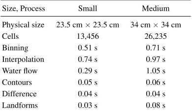
19 Table 2.2

Scanning speed for different model sizes .

.

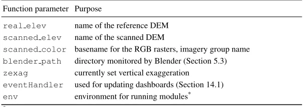
25 Table 2.3

Available parameters of functions ran for each scan

.

29 Table 2.4

Classes of the Anderson fuel model

.

75 Table 2.5

Overview of design stages and their associated interaction modes

.

87 Table 3.1

The amount of simulated rainfall water

.

102 Table 4.1

List of selected predictors and estimated coefficients for site suitability .

.

110

(10)

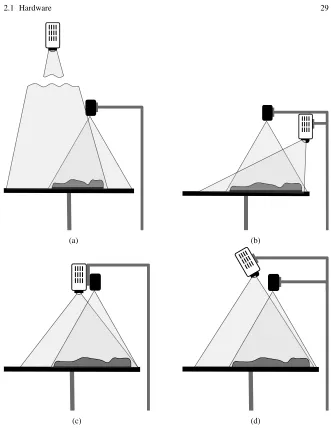
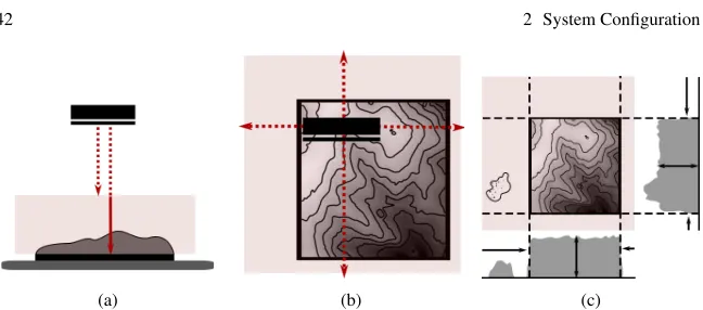
Figure 2.1

Possible placements of the projector and scanner

.

15 Figure 2.2

Mobile system setup

.

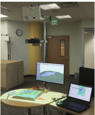
17 Figure 2.3

Laboratory system setup

.

18 Figure 2.4

Calibration of angular deviation .

.

22 Figure 2.5

Accuracy assessment

.

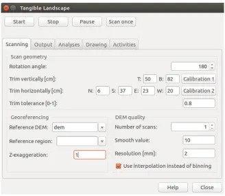
26 Figure 2.6

Tangible Landscape plugin dialog

.

27 Figure 2.7

Finding the boundaries of the physical model

.

28 Figure 2.8

Different modes of interaction used in Tangible Landscape .

.

33 Figure 2.9

Examples of different tangible objects used for interaction

.

33 Figure 2.10

3D sketching a levee breach with feedback on the resulting extent of flooding

.

33 Figure 2.11

Schema of interaction with 3D rasters

.

34 Figure 2.12

Exploring 3D soil moisture dataset

.

35 Figure 2.13

Examples of using markers .

.

36 Figure 2.14

Using magnetized markers on a CNC-routed model with magnetic primer

.

36 Figure 2.15

Examples of using markers to explore 3D soil moisture distribution

.

37 Figure 2.16

Calibration and scanning of colored felt pieces .

.

39 Figure 2.17

Using colored sand to design new urban development zones in Asheville

.

40 Figure 2.18

Using the direction of the marker to change azimuth of the sun for shaded relief

computation .

.

42 Figure 2.19

Using the position and direction of the marker to compute visibility

.

43 Figure 2.20

Flow accumulation and watershed boundaries

.

48 Figure 2.21

Water depth computed with r.sim.water

.

49 Figure 2.22

An overview of Lake Raleigh’s surroundings .

.

50 Figure 2.23

Detailed view of the sand model in the dam location

.

52 Figure 2.24

The flood simulation with current conditions

.

52 Figure 2.25

The flood simulation after the road has been removed

.

53 Figure 2.26

The study area with extent of the physical model

.

54 Figure 2.27

A physical model of landscape with projected orthophoto, contours, and

sim-ulated water flow depth

.

55 Figure 2.28

Line of sight analysis

.

57 Figure 2.29

Lake Raleigh Woods DSM

.

58 Figure 2.30

Placing a marker to identify a viewpoint

.

59 Figure 2.31

Viewsheds computed on lidar-based DSM

.

60 Figure 2.32

Modeling viewsheds from a new building

.

60 Figure 2.33

View of the new hotel building from Lake Raleigh dam

.

61 Figure 2.34

The TSP applied to a network of potential trails

.

65 Figure 2.35

The slope and cross-slope of a trail

.

65 Figure 2.36

Friction map for Lake Raleigh

.

68

(11)

Figure 2.43

The spread of fire after creating a firebreak .

.

81 Figure 2.44

The simulation with additional firebreak

.

82 Figure 2.45

Tangible Landscape setup for design case study

.

85 Figure 2.46

Study area with the highlighted physical model extent

.

88 Figure 2.47

First scenario: sculpting the landscape

.

89 Figure 2.48

First scenario: planting and siting the shelter .

.

91 Figure 2.49

Second scenario: sculpting the landscape, planting and siting the shelter

.

92 Figure 2.50

A comparison of two design scenarios

.

94 Figure 3.1

Schema of DEM fusion

.

99 Figure 3.2

Study area

.

100 Figure 3.3

Spatially variable overlap width

.

101 Figure 3.4

Terrain profile of fused and source DEMs .

.

101 Figure 3.5

Effect of DEM fusion on water flow patterns .

.

102 Figure 3.6

Tangible Landscape .

.

103 Figure 4.1

Simplified schema of F UTURES conceptual model .

.

107 Figure 4.2

Diagram of F UTURES workflow .

.

108 Figure 4.3

An example of r.futures.demand output plot

.

108 Figure 4.4

2011 land cover and protected areas in the Asheville metropolitan area

.

109 Figure 4.5

Results of three realizations of multiple stochastic runs with different scenarios

110 Figure 4.6

Area in km

2

of converted land from forest and farmland to urban

.

110 Figure 5.1

Tangible Landscape setup

.

116 Figure 5.2

Steering framework architecture

.

119 Figure 5.3

Pilot workshop

.

121 Figure 5.4

Simulated spread of Sudden Oak Death without any intervention

.

124 Figure 5.5

Simulated spread of Sudden Oak Death with adaptive management

.

125 Figure 5.6

Workflow diagram

.

126

(12)

CHAPTER

1

Introduction

1.1 Motivation

With the rise of computer technology and ubiquitous sensors in the past several decades, geospatial

modeling and analysis has penetrated the traditional scope of many disciplines and became an integral

part of many interdisciplinary research endeavors. With advanced visualizations and 3D displays we

can now better explore and experience data and processes visually, however the manipulation of 3D

geospatial data is still limited [Piper et al., 2002a; Ratti et al., 2004]. When using a mouse, keyboard,

and digital display we are separated from our data by multiple layers of abstraction, making the

inter-action unintuitive [Sharlin et al., 2004] and hindering collaboration. Moreover, traditional interfaces

to geospatial models typically assume familiarity with the software as well as a basic understanding

of spatial concepts and representations, which creates barriers to the engagement of non-experts

[Ab-bot et al., 1988; Rambaldi, 2010]. However, collaboration between non-experts and researchers from

different fields is recognized as essential for making progress towards solving today’s complex

envi-ronmental issues [Voinov & Bousquet, 2010].

(13)

The recent advances in remote-sensing technologies have opened new ways to harness the

poten-tial of physical models as collaborative environments for learning and problem solving. Coupling the

physical and digital models through a real-time cycle of interaction, 3D scanning, computation, and

projection allows for the physical manifestation of geospatial data and promotes accelerated

learn-ing, prototyplearn-ing, and the exchange of ideas. While the concept of tangible geospatial modeling offers

numerous opportunities to advance interdisplinary research, it also raises many questions about its

implementation and applications, which have not been explored before.

1.2 Background

With the advancement of scanning technology, multiple research groups have developed approaches

to couple physical and digital models to create a collaborative environment for intuitive design and

decision making augmented with geospatial analyses. The MIT Media Lab developed the early

proto-types of these continuous shape displays—Illuminating Clay [Piper et al., 2002a] and Sandscape [Ishii

et al., 2004]—which link a continuous physical model with its digital representation through a cycle of

sculpting, 3D scanning, computation, and projection. The coarse resolution of these systems, given by

the sensing technology and the physical medium, was not suitable for representing real landscapes.

Both systems used a limited library of custom implementations of geospatial analyses, which led to

the idea of integration with a full GIS, giving the users wide range of sophisticated, scientific tools

for modeling and visualization [Piper et al., 2002b]. The Tangible Geospatial Modeling System

(Tan-GeoMS) adopted this approach and extended the concept of Illuminating Clay by integration with

GRASS GIS and working with real landscapes [Tateosian et al., 2010]. However, establishing a near

real-time connection between a laser scanner and a GIS proved challenging.

(14)

In my dissertation I explore the emerging concept of tangible geospatial modeling from its

technolog-ical foundations to its practtechnolog-ical applications in various domains. In the second chapter of this thesis I

describe the methodology developed behind Tangible Landscape, which is the first system with

real-time coupling of a 3D physical model with a Geographic Information System (GIS), namely GRASS

GIS, an open source geospatial platform. This chapter specifically describes the method to couple a 3D

physical model with a georeferenced digital model to enable interaction with real geospatial data and

algorithms at relevant extents and scales. To explore the potential of tangible geospatial modeling, I

developed various interaction methods using tangible objects, allowing users to intuitively create new

geospatial inputs into models. The ability to interact with elevation surfaces, cross-sections, different

types of vector geometries directionality, or categorical data helped me to develop a wide range of

applications, which are described in the second chapter.

When designing a tangible modeling application we need to consider the scale of the interaction

for realistic landscape modifications, which then directly influences the size and scale of our physical

model. The spatial extent of the modeled phenomena, however, often does not match the extent of

the physical model. Modeled processes such as wildfire or disease spread can originate outside of the

physical model’s extent, and spread beyond it. Similarly, overland flow is spatially defined by watershed

boundaries, which typically do not match the scale of our interactions on the physical model. This can,

for example, lead to the inability to properly model the effects of our interventions on the water flowing

downstream outside of the model’s boundaries. The possible solution for these cases is to perform the

computations on a larger extent while merging the interventions on the physical model into one larger

digital elevation model (DEM). The third chapter generalizes this problem into the question of how to

create a seamless digital elevation model from partially overlapping DEMs from different sources while

preserving their topographic features. Apart from the tangible geospatial modeling context, this is an

increasingly common problem due to the growing availability of lidar- and UAS-based datasets with

different extents, and spatial and temporal resolutions. The developed method addresses this problem

in a fast and effective manner, and thanks to its GIS-based implementation, it can be easily integrated

into common DEM processing workflows, enhancing the subsequent modeling results.

(15)

completely removes these barriers. F UTURES is now being tested and applied by the land change

community for different extents and urbanization patterns, leading to a more robust model.

While making a complex spatio-temporal model accessible to the scientific community is

challeng-ing, bringing it to practitioners and stakeholders to inform decisions on natural resource managment

issues is typically even more difficult. Thanks to its visualization capabilities, an intuitive interface, and

strong geospatial component, tangible geospatial modeling is highly suited for facilitating discussions

among stakeholders and decision makers. In the final chapter of my dissertation I couple a dynamic,

spatially-explicit epidemiological simulation of a tree disease called Sudden Oak Death with

Tangi-ble Landscape to create a unique participatory modeling tool, where stakeholders can explore

differ-ent managemdiffer-ent scenarios through the steering of the simulation. The proposed generalized steering

framework makes this deployment of Tangible Landscape applicable to other dynamic models such as

wildfire, or urban growth simulations.

(16)

CHAPTER

2

Tangible Modeling with Open Source GIS

Reprint

Anna Petrasova, Brendan A. Harmon, Vaclav Petras, Payam Tabrizian and Helena Mitasova. 2018.

Tangible Modeling with Open Source GIS. Springer International Publishing. 2nd edition (in press).

This thesis contains selected chapters of the book.

Attribution

(17)

Anna Petrasova, Brendan Harmon, Vaclav

Petras, Payam Tabrizian, Helena Mitasova

Tangible Modeling with Open

Source GIS

March 12, 2018

(18)

1 Introduction. . . 1

1.1 Tangible User Interfaces . . . 1

1.2 Tangible Geospatial Modeling . . . 4

1.2.1 Shape Changing Interfaces . . . 5

1.2.2 Augmented Architectural Interfaces . . . 8

1.2.3 Augmented Clay Interfaces . . . 9

1.2.4 Augmented Sandbox Interfaces . . . 10

1.3 Tangible Landscape . . . 13

1.3.1 Developing Tangible Landscape . . . 16

1.4 The Organization of This Book . . . 16

References . . . 20

2 System Configuration. . . 25

2.1 Hardware . . . 25

2.1.1 3D Scanner . . . 25

2.1.2 Projector . . . 27

2.1.3 Computer Requirements . . . 28

2.1.4 Physical Setup . . . 28

2.2 Software . . . 32

2.2.1 GRASS GIS . . . 33

2.2.2 GRASS GIS Python API . . . 34

2.2.3 Scanning Module r.in.kinect . . . 35

2.2.4 Tangible Landscape Plugin for GRASS GIS . . . 39

2.2.5 Tangible Landscape Plugin Installation . . . 44

References . . . 44

3 Building Physical 3D Models . . . 47

3.1 Handmade Models . . . 47

3.2 Digitally Fabricated Models . . . 49

3.2.1 Digital Models . . . 50

(19)

3.2.3 CNC Routing . . . 53

3.2.4 3D Printing . . . 58

3.3 Molding and Casting . . . 58

3.4 Workflows . . . 60

3.4.1 Selecting a 3D Model Scale . . . 61

3.4.2 Sculpting a Malleable Model from Lidar Data . . . 63

3.4.3 CNC Routing a Topographic Model from Contour Data . . . . 64

3.4.4 CNC Routing Topographic and Surface Models from Lidar Data . . . 64

3.4.5 3D Printing Topographic and Surface Models from Lidar Data . . . 66

3.4.6 Casting a Malleable Topographic Model with a CNC Routed Mold Derived from Lidar Data . . . 67

References . . . 68

4 Tangible Interactions . . . 69

4.1 Modes of Interaction . . . 69

4.2 3D Sculpting of Surfaces and Volumes . . . 70

4.3 Detecting Markers . . . 71

4.4 Detecting Color and Shape . . . 74

4.5 Combining Color and Elevation . . . 76

4.6 Direction Marker . . . 78

References . . . 80

5 Real-time 3D Rendering and Immersion. . . 81

5.1 Blender . . . 81

5.2 Hardware and Software Requirements . . . 82

5.3 Software Architecture . . . 83

5.4 File Monitoring . . . 83

5.5 3D Modeling and Rendering . . . 84

5.5.1 Handling Geospatial Data . . . 85

5.5.2 Object Handling and Modifiers . . . 86

5.5.3 3D Rendering . . . 88

5.5.4 Materials . . . 90

5.6 Workflows . . . 92

5.7 Realism and Immersion . . . 95

5.7.1 Realism . . . 95

5.7.2 Virtual Reality Output . . . 96

5.8 Tangible Landscape Add-on in Blender . . . 97

References . . . 98

6 Basic Landscape Analysis. . . 101

6.1 Processing and Analyzing the Scanned DEM . . . 101

6.1.1 Creating DEM from Point Cloud . . . 101

(20)

6.1.3 Analyzing the DEM . . . 103

6.2 Case Study: Topographic Analysis of Graded Landscape . . . 106

6.2.1 Site Description and 3D Model Properties . . . 107

6.2.2 Basic Workflow with DEM Differencing . . . 107

6.2.3 The Impact of Model Changes on Topographic Parameters . 109 6.2.4 Changing Landforms . . . 111

References . . . 112

7 Surface Water Flow Modeling . . . 113

7.1 Foundations In Flow Modeling . . . 113

7.1.1 Overland Flow . . . 113

7.1.2 Dam Breach Flooding . . . 115

7.2 Case Study: The Impact of Development on Surface Water Flow . . . 116

7.3 Case Study: Dam Breach . . . 118

7.3.1 Site Description and Input Data Processing. . . 119

7.3.2 The Impact of the Road on Flooding . . . 120

7.4 Case Study: Flow Outside the 3D Model Area . . . 121

7.4.1 Site Description and the Physical Model . . . 122

7.4.2 Surface Runoff Modeling . . . 122

8 Soil Erosion Modeling . . . 125

8.1 Soil Erosion and Deposition Modeling . . . 125

8.2 Case Study: Designing Erosion Control Measures . . . 126

8.2.1 Site Description and 3D Model Properties . . . 127

8.2.2 Erosion Modeling While Modifying Topography . . . 128

8.2.3 Reducing Erosion by Modifying Land Cover . . . 129

9 Viewshed Analysis . . . 133

9.1 Line of Sight Analysis . . . 133

9.2 Case Study: Viewsheds around Lake Raleigh . . . 134

9.2.1 Site Description and Model . . . 134

9.2.2 Visibility Analysis on DSM Using Markers . . . 135

9.2.3 Modeling Viewsheds from a New Building . . . 136

10 Trail Planning . . . 139

10.1 Trail Design Methodology . . . 139

10.1.1 Least Cost Path Analysis . . . 140

10.1.2 Network Analysis . . . 141

10.1.3 Trail Slope Extraction . . . 141

10.2 Case Study: Designing a Recreational Trail . . . 143

10.2.1 Input Data Processing . . . 143

10.2.2 Computing the Trail Using the Least Cost Path . . . 144

(21)

10.2.4 Mapping Trail Slopes . . . 147

10.2.5 Alternative Trail Scenarios . . . 150

11 Solar Radiation Dynamics . . . 151

11.1 Solar Radiation Modeling . . . 151

11.2 Case Study: Solar Irradiation in Urban Environment . . . 153

11.2.1 The Impact of Building Configuration on Cast Shadows . . . . 154

11.2.2 The Impact of Building Configuration on Direct Solar Irradiation . . . 154

12 Wildfire Spread Simulation . . . 159

12.1 Fire Spread Modeling Methods . . . 159

12.1.1 Input Data . . . 159

12.1.2 Fire Spread Algorithm . . . 160

12.2 Case Study: Controlling Fire with Firebreaks . . . 161

12.2.1 Data Preparation . . . 162

12.2.2 Scenario with Multiple Firebreaks . . . 163

13 Coastal Modeling . . . 169

13.1 Modeling Potential Inundation . . . 169

13.2 Case Study: Simulating Barrier Islands Flooding . . . 170

13.2.1 Storm Surge Flooding at Jockey’s Ridge Sand Dunes . . . 170

13.2.2 Exploring Storm Surge Protection . . . 172

13.3 Case Study: Designing Resilient Coastal Architecture . . . 174

14 Landscape Design. . . 177

14.1 Integrating Tangible and 3D Modeling Methods . . . 177

14.2 Case Study: Designing a Park . . . 181

14.2.1 Site Description and Model . . . 181

14.2.2 Scenario 1 . . . 182

14.2.3 Scenario 2 . . . 183

14.2.4 Evaluation of Scenarios . . . 183

A Appendix . . . 189

A.1 Applications of Tangible Landscape . . . 189

A.2 Data Sources . . . 198

A.3 Starting with GRASS GIS . . . 200

(22)

System Configuration

The setup of the Tangible Landscape system consists of four primary components: (a) a physical model that can be modified by a user, (b) a 3D scanner, (c) a pro-jector, and (d) a computer installed with GRASS GIS for geospatial modeling and additional software that connects all the components together. The physical model, placed on a table, is scanned by the 3D scanner mounted above. The scan is then imported into GRASS GIS, where a DEM is created. The DEM is then used to compute selected geospatial analyses. The resulting image or animation is projected directly onto the modified physical model so that the results are put into the context of the modifications to the model.

2.1 Hardware

Tangible Landscape can be built with affordable, commonly available hardware: a 3D scanner, a projector and a computer. We describe some of the current hardware options, while noting that the technology develops rapidly, and alternative, more effective solutions may emerge.

2.1.1 3D Scanner

(23)

The Technology Behind 3D Scanning We describe the basic principles behind current 3D depth sensing technologies, with just enough detail to explain both the potential and the limitations of current scanning devices. More detailed information can be found, for example, in Mutto et al. (2012).

Several currently available depth sensors such as Apple Primesense Carmine, Asus Xtion PRO LIVE1_{, and Kinect for Windows v1, are based on a Primesense} proprietary light-coding technique. This technique uses triangulation to map 3D space in a manner similar to how the human visual system senses depth from two slightly different images. Rather than using two cameras, it triangulates between a near-infrared camera and a near-infrared laser source. Corresponding objects need to be identified in order to triangulate between the images. A light coding (or structured light) technique is used to identify the objects. The laser produces a pseudo-random dot pattern which is then used to find the matching dot pattern in the projected pattern. In this way, the final depth image can be constructed.

Kinect for Xbox One usesTime-of-Flight(ToF), a technique widely used in lidar technology. It has a sensor that indirectly measures the time it takes for pulses of near-infrared laser light to travel from a laser source, to a target surface, and then back to the image sensor. Time-of-Flight sensors are generally considered to be more precise, but are also more expensive.

Since the scanning and 3D modeling algorithms and their implementations for most sensors are proprietary, the specific behavior and precision of particular sen-sors is the subject of many experimental studies. Generally, sensen-sors using near-infrared light are sensitive to lighting conditions, so outdoor usage is typically not recommended. The depth resolution decreases with the distance from the sensor and also at close range (i.e. between a couple of millimeters to tens of centimeters). The range and field of view of the sensors can vary; Tangible Landscape requires short range sensors with a minimum distance of 0.5 m to keep the highest possible res-olution. When scanning with one sensor, the size of the physical model is limited by the required accuracy because the sensor must be far enough away to capture the entire model in the sensor’s field of view, which for the Kinect for Xbox One is 60° vertical by 70° horizontal.

Detailed information about accuracy and precision of Kinect for Windows v1 and Kinect for Xbox One can be found in Wasenm¨uller and Stricker (2017); Andersen et al. (2012); Lachat et al. (2015) and a comparison to Asus Xtion can be found in Gonzalez-Jorge et al. (2013). The main factors that limit the accuracy of Kinect for Xbox One include the correlation of depth accuracy and scanner temperature, the influence of scene color on depth estimation, flying pixels (erroneous pixels, a well-known artifact of ToF cameras) along depth discontinuities, and high depth deviation in image corners. Knowing these limitations, we can to a certain extent compensate for them by pre-heating the scanner before measuring, avoiding high contrast scenes, and using statistical filtering methods to avoid flying pixels (see Section 2.2.3 for more details).

(24)

2.1.2 Projector

The projector projects the background geospatial data and results of analyses onto the 3D physical model. Therefore, it is important to select a projector with sufficient resolution and properties that minimize distortion and generate a bright image.

Resolution and brightness are two important criteria to be considered. We recom-mend higher resolution projectors offering at least WXGA (1280×800). The bright-ness depends upon where Tangible Landscape is used and whether the room’s am-bient light can be reduced for the sake of brighter projected colors. We recommend brighter projectors (at least 3000 lumens) since we project on a variety of materials which are not always white and reflective.

There are two main types of projectors — standard and short-throw projectors. They differ in throw ratio values, which are defined as the distance from the projec-tor’s lens to the screen, divided by the width of the projected image (short throw and ultra short throw projectors have ratios 0.7 - 0.3, while the standard projectors have throw ratio values around 2). At the same distance the projector with a lower throw ratio can display a larger image. In other words, a projector with a lower throw ratio (short-throw) can project an image of the same size as the higher throw ratio projec-tor, but from a shorter distance. Tangible Landscape can be set up using both types of projectors; each has advantages and disadvantages.

The placement and configuration of the projector is important because it affects the coverage, distortion, and visibility of the projected data. For example, in some setups the 3D scanner may be caught in the projection and would thus cast a shadow over the model. Therefore it can be practical to use a short-throw projector because it can be placed to the side of the physical model at a height similar to the 3D scan-ner (Fig. 2.1b and 2.3). Since the projection is cast from the side, the projection beam does not cross the 3D scanning device and no shadow is cast. However, with a short-throw projector there is a certain level of visible distortion when project-ing on a physical model that has substantial relief. The distortion occurs because the light rays reach the model at an acute angle. The horizontal position at which the projected light intersects the model is shifted from the position at which it would intersect with a flat surface. Larger differences in height increase the distortion. The-oretically, we can remove the distortion by either warping the projected data itself or using the projector to automatically warp the projected image. The first solution would require an undistorted dataset for geospatial modeling and a warped copy of that data for projecting. That is impractical, especially when working with many different raster and vector layers. The other solution requires the projector itself to warp the image; while this technology exists, it is only offered by a few projector manufacturers and such projectors are typically more expensive. Moreover, as the landscape is modified, the warping pattern should change as well. Currently it is not possible to find this feature in the off-the-shelf projectors.

(25)

manipulate the projector when is it so high above the model. Furthermore it is chal-lenging to align the projector and the 3D scanner without casting a shadow. Since the 3D scanner has a limited field of view it must be placed close to the horizontal center of the model. When the projector is mounted above the scanner, the scanner is caught in the projector’s beam, casting a shadow over part of the model. For small to mid sized models, depending on the particular setup and the height of the scanner and projector, this may not be a problem.

The shadow of the scanner can also be avoided with specialized short throw pro-jectors that allow greater installation flexibility through lens shifting. These projec-tors (for example Canon WUX400ST) are capable of projecting from the horizontal center of the projected area at the same height as the scanner (Fig. 2.1c). A device which combines the scanner and projector would make this setup easy; an appropri-ate device, however, was not available at the time of writing.

To minimize the distortion when using projectors with lower throw ratios, we can project from the center by tilting the projector and correcting the resulting keystone distortion (Fig. 2.1d). With this setup we recommend projectors that have throw ratios around 1.0 (for example Epson PowerLite 1700 Series) as a lower ratio can result in additional distortion. When testing the projector setup it is useful to project the rectangular grid on a flat surface in order to quickly check if there is any distor-tion.

2.1.3 Computer Requirements

System requirements depend largely upon the sensor and its associated library or software development kit (SDK). Certain sensors, such as Kinect for Xbox, are designed to work on specific operating systems with the producer’s SDK, how-ever open source drivers, namelylibfreenect2(Xiang et al., 2016), allow users to run Kinect on other platforms. The preferred platform of Tangible Landscape is GNU/Linux distribution Ubuntu, see notes in Section 2.2.5. The computer should be configured for 3D scanning and geospatial modeling, both of which are performance-and memory-intensive processes. The hardware requirements are very similar to the requirements for gaming computers: a multi-core processor, at least 4 GB of sys-tem memory and a good graphics card are necessary to achieve real-time interaction with the model. The specific parameters required for the scanner device should be reviewed on the manufacturer’s website.

2.1.4 Physical Setup

(26)

build-(a) (b)

(c) (d)

(27)

ing Tangible Landscape in the laboratory or when bringing it to the community, the following items are necessary:

• a table for a model

• a laptop or desktop computer with a table • a scanner

• a projector

• 1-2 stands for a projector and a scanner • 3-4 power plugs (and/or extension cable)

Ideally the table should be either a 90 cm×90 cm square table with rounded cor-ners, a rounded table 100 cm in diameter, or a teardrop table of similar size. To freely interact with the model a person should be able to almost reach the other side of the table; this is not possible with larger tables. Smaller tables, on the other hand, have less space for tools, additional sand, and application windows. Ideally application windows with additional information should be projected onto the table beside the model. A large model can be placed on top of a smaller table or stand, provided that this base is stable. In this case, if any application windows are needed, they have to be projected directly onto the model.

A round table is quite advantageous because people can stand at equal distances from the model and can easily move around the table. Unfortunately, one side of the table is typically occupied by the metal stands for projector and scanner since ceil-ing mounts are rarely possible and render the system immobile. The table should be stable enough to hold sand and models and sturdy enough to withstand their manipu-lation. We recommend putting the computer on a separate table so that the modeling table is not cluttered. The more space there is around the modeling table, the more access users have to the model. The computer, however, needs to be situated so that its operator has easy access to the model as well.

An alternative is to use a rectangular table (ideally with rounded corners) that is 140 cm×90 cm for both the model and the laptop. A narrow table that is 150 cm×75 cm may work as well. This setup makes the model less accessible as at least two sides of the model are blocked. However, the whole model should be accessible from any of the remaining sides, so this setup does not necessarily limit interaction, but rather the number of users.

Sometimes it is advantageous to have a large screen showing additional data or 3D views to enhance users’ understanding of the processes. However, such a screen should not limit access to the physical model. Tangible Landscape could also be extended with additional devices such as 3D displays, head-mounted displays, and hand-held devices.

(28)

Fig. 2.2 Mobile system setup: projector, scanner, model, laptop and optionally screen.

(29)

Fig. 2.3 Laboratory system setup with short throw projector and large physical model.

stand. Fig. 2.3 shows a similar setup with a short throw projector. For permanent setups the projector can be mounted on the ceiling.

2.2 Software

The software for Tangible Landscape consists of two main components:

• Moduler.in.kinectis a GRASS GIS module which obtains depth and optionally color data from Kinect sensor and processes it into a DEM and RGB rasters. It can run in a loop to continually create new DEMs.

• Tangible Landscape Plugin is a GUI plugin of GRASS GIS, which callsr.in.kinect and runs selected geospatial analyses on the scanned DEMs as the physical model is being scanned.

(30)

Tangible Landscape software is available in the GitHub repository2 _{under the} GNU GPL license.

2.2.1 GRASS GIS

GRASS GIS (Neteler and Mitasova, 2008) is a general purpose cross-platform, open-source geographic information system with raster, vector, 3D raster, and im-age processing capabilities. It includes more than 400 modules for managing and analyzing geographical data and many more user contributed modules available in the add-on repository. GRASS GIS modules can be run using a command-line in-terface (CLI) or a native graphical user inin-terface (GUI) called wxGUI, which offers a seamless combination of GUI and CLI native to the operating system.

Modules are organized based on the data type they handle and they follow nam-ing conventions explained in Table 2.1. Each module has a set of defined options and flags, which are used to specify inputs, outputs, or different module settings. Most core modules using GRASS GIS C library are written in C for performance and portability reasons. Other modules and user scripts are written in Python, us-ing the Python Scriptus-ing Library which provides a Python interface to GRASS GIS modules.

Table 2.1 Naming conventions for GRASS GIS modules with examples.

Name Data type Examples

g.* general data management g.list, g.remove, g.manual r.* raster data r.neighbors, r.viewshed, r.cost r3.* 3D raster data r3.colors, r3.to.rast, r3.cross.rast v.* vector data v.net, v.surf.rst, v.generalize db.* attribute data db.tables, db.select, db.dropcolumn t.* temporal data t.register, t.rast.aggregate, t.vect.extract i.* imagery data i.segment, i.maxlik, i.pca

GRASS GIS software can be downloaded freely from the main GRASS project website.3_{The download web page offers easy to install binary packages for GNU/Linux,} Mac OS X, and Microsoft Windows as well as the source code. The GRASS GIS website also provides additional documentation, including manual pages, tu-torials, information about the externally developed modules (add-ons) and vari-ous publications. Support for developers and users is provided by several