ABSTRACT
COONLEY, BRETT WILLIAM. Sequential Programming for PDE Constrained Optimizations. (Under the direction of Kazufumi Ito.)
Sequential Progamming (SP) is a method for solving PDE constrained optimizations. These include many applications of practical importance, especially optimal control problems, such as the optimal control of fluid flow governed by the incompressible Navier-Stokes equations. The Sequential Programming (SP) method is guaranteed to converge to an optimizer of a PDE constraint problem under proper conditions. A hallmark of the method is that there is no line search needed for the damped update involved in sequential iterations.
Sequential Programming for PDE Constrained Optimizations
by
Brett William Coonley
A dissertation submitted to the Graduate Faculty of North Carolina State University
in partial fulfillment of the requirements for the Degree of
Doctor of Philosophy
Mathematics
Raleigh, North Carolina 2015
APPROVED BY:
Zhilin Li Xiao-Biao Lin
Hien Tran Kazufumi Ito
DEDICATION
BIOGRAPHY
The author was born in New Hampshire where he attended the Montessori School. He moved to Connecticut and attended Union Elementary School, Lake Garda Elementary School, Har-Bur Middle School, and graduated valedictorian of Lewis S. Mills High School in 1995. He was a member of the high school Math Team during 8th grade through senior year when he was President and MVP of the team. He was voted DAR Good Citizen by his high school class, performed classical piano in the high school talent show, qualified for the State Wrestling Championships, and was a Boy Scout in Troop 37 of Unionville.
ACKNOWLEDGEMENTS
My greatest thanks of all go to my advisor Dr. Kazufumi Ito for his guidance and dedication. Dr. Ito showed me patience, kindness, and persistence, and instilled in me a drive to reach for more than I need.
I would also like to thank my committee members Dr. Zhilin Li, Dr. Xiao-Biao Lin, and Dr. Hien Tran for being available and encouraging. Each of you has unique skill and talents that have shaped and improved my work.
Special thanks go to my colleagues Amanda Landi and Melissa Ngamini, and my good friend Ryan Patridge.
TABLE OF CONTENTS
LIST OF TABLES . . . vii
LIST OF FIGURES . . . .viii
Chapter 1 Introduction . . . 1
Chapter 2 Optimization Theory. . . 4
2.1 Constrained Optimization . . . 4
2.2 Unconstrained Non-smooth Minimization . . . 5
2.2.1 Existence of Minimizers . . . 6
2.2.2 Necessary Optimality . . . 6
2.2.3 Deconvolution Problem . . . 8
2.2.4 Inverse Medium Problem . . . 9
2.3 Lagrange Multiplier Theory . . . 9
2.3.1 Equation Form of Complementarity Condition . . . 11
2.4 Optimal Control Problem . . . 12
2.4.1 Necessary Optimality . . . 14
Chapter 3 Sequential Programming Method and Theory . . . 16
3.1 Lagrange Calculus . . . 17
3.2 Gradient Method . . . 19
3.3 Sequential Quadratic Programming (SQP) . . . 20
3.4 Sequential Programming . . . 22
3.4.1 Convergence . . . 22
3.4.2 Second Order Sequential Programming Method . . . 26
3.4.3 Fixed Point Formulation of Saddle Point Problem . . . 27
3.4.4 Second Order Version . . . 28
3.4.5 Non-smooth Cost Case . . . 28
3.4.6 Properties . . . 29
3.5 Bilinear Control Problem and Partial SQP . . . 29
3.6 Saddle Point Solver . . . 30
3.6.1 Reduced Order CG . . . 31
3.6.2 Preconditioned Conjugate Residual (CR) Method . . . 32
3.6.3 Inequality Case . . . 33
3.7 Comparison to Gradient Method and SQP . . . 35
Chapter 4 Applications of SP . . . 37
4.1 Optimal Control Problem . . . 37
4.2 Ill-posed Inverse Problem . . . 38
4.3 Semilinear Control Problem . . . 39
4.3.1 Moving Damping Actuator Control Problem . . . 42
4.4 Non-smoothness in SP . . . 45
4.4.2 Newton-like Solver . . . 47
4.4.3 Inequality Constraint . . . 48
Chapter 5 Optimal Control of Navier-Stokes System and SP . . . 50
5.1 Navier-Stokes Control Problem . . . 50
5.1.1 Stokes Theory . . . 52
5.1.2 Hodge Decomposition . . . 53
5.1.3 Weak Solution of Navier-Stokes . . . 54
5.1.4 Optimal Control Problem for Incompressible Navier-Stokes Flow . . . 56
5.2 Optimality System . . . 57
5.3 SP for Navier-Stokes Control . . . 58
5.4 Numerical Methods . . . 59
5.4.1 Gradient of Pressure . . . 60
5.4.2 Divergence of Velocity . . . 60
5.4.3 Convective Term . . . 62
5.4.4 Diffusion Term . . . 63
5.4.5 Second Order Implicit–Explicit Time Integration Method . . . 65
Chapter 6 Discretization in Time and Space . . . 67
6.1 Application of SP for Optimal Control Problem . . . 68
6.1.1 High Order Discretized Problem . . . 68
6.1.2 Runge-Kutta-Gauss Method . . . 69
6.1.3 Necessary Optimality for Discretized Control Problem . . . 71
6.1.4 Discretized Saddle Point Problem for SP . . . 72
6.1.5 Saddle Point Solver and Preconditioner . . . 73
Chapter 7 Concrete Examples and Numerics . . . 75
7.1 Lorenz Attractor With Control . . . 75
7.1.1 Implementation of Controlled Lorenz Problem . . . 78
7.1.2 Cost and Convergence Study . . . 82
7.1.3 Parameter Study for Controlled Lorenz Problem . . . 84
7.1.4 The Code Tpbdry.m . . . 85
7.2 Coefficient Optimal Control in Elliptic Equations . . . 91
7.3 Moving Damping Actuator Control Problem . . . 93
7.4 Tests for Numerical Method for Controlled Navier-Stokes System . . . 94
Chapter 8 Summary and Conclusion . . . 96
References. . . 98
Appendix . . . .104
LIST OF TABLES
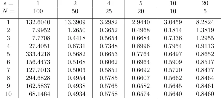
Table 7.1 Cost JN(uN) for varying numbers of stages s and subintervals N over 10
iterations. . . 83 Table 7.2 Computation of |x(T)−xtarget|2 for varying numbers of stagess and
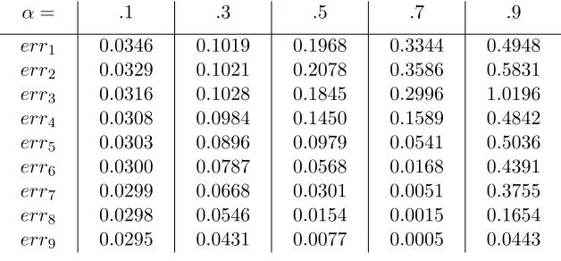
subin-tervals N over 10 iterations. . . 83 Table 7.3 Relative error errn+1 = |xn+1−xn|/|xn| between state iterates for varying
(damping) stepsizes α = .1, .3, .5, .7, .9 over 10 iterations, with s = 5 stages and N = 20 subintervals. . . 84 Table 7.4 Convergence rates rn = errn+1/errn corresponding to iterates in Table 7.3
LIST OF FIGURES
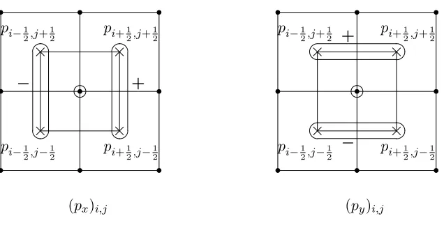
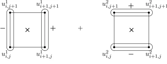
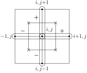
Figure 5.1 Two-dimensional staggered grid for step flow withh×hsquare cells,h= 1/4. Pressure nodes ×at cell centers and velocity nodes •at cell corners. . . 59 Figure 5.2 Gradient term ∇p= (px, py) located at i, j grid node. . . 61
Figure 5.3 Divergence term divu=u1
x+u2y located ati, j pressure node. . . 62
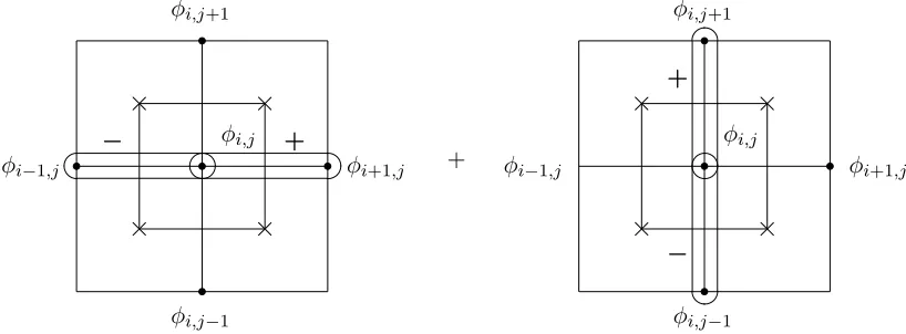
Figure 5.4 Convective termu· ∇φ(with φ=u1 or u2) located at i, j grid node. . . 63 Figure 5.5 Diffusion (Laplace) term −∆u = (−∆u1,−∆u2) located at i, j grid node.
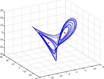
(φ=u1 for−∆u1 and φ=u2 for −∆u2.) . . . 64 Figure 7.1 Lorenz attractor with parameters σ = 4, ρ = 50, β = 1 exhibits a butterfly
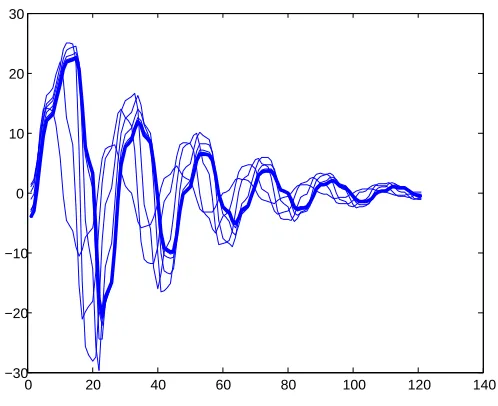
shape. . . 76 Figure 7.2 Iterates x1, . . . , x10 by Tpbdry.m for the controlled Lorenz system.
Parame-ters β = 1, c = 1 over time horizon [0,5] with 5 stages and 20 subintervals, targeting equilibrium (7,7,−1) with initial conditionx0 = (1,1,1) and damp-ing parameter α=.7. . . 79 Figure 7.3 Controlsu1, . . . , u10 corresponding to states x1, . . . , x10 in Figure 7.2. . . 81 Figure 7.4 Controluafter 10 iterations for varying number of subintervals N = 20,40,80. 81 Figure 7.5 Orbit ofx0 = (1,1,1) and corresponding controlufor varied control authority
parameter β = 1,101,1001 . (Other parameters α = .7 and c = 1, over time horizon [0,5].) . . . 86 Figure 7.6 Effect on control u of varying terminal timeT = 5,2,1. . . 86 Figure 7.7 Effect on orbit ofx0 of varying target authority parameter c= 101 ,1,10. . . . 86 Figure 7.8 Optimal control u satisfying |un+1−un|
|un| <10
Chapter 1
Introduction
In this thesis we consider constraint optimization problems in Hilbert spaces. Optimization is one of the key components for mathematical modeling of real world problems and the solu-tion method provides an accurate and essential descripsolu-tion and validasolu-tion of the mathematical model. Optimization problems are encountered frequently in engineering and sciences and have widespread practical applications. An appropriately chosen cost functional is minimized sub-ject to constraints. For example, the constraints are in the form of equality constraints and inequality constraints. We also discuss a class of non-smooth optimizations. A non-smooth op-timization method is a very basic modeling tool and enlarges and enhances the applications of the optimization method in general. For example in imaging/signal analysis the sparsity optimization is used by means of L1 and T V norm regularization.
A sequential algorithm based on Sequential Programming (SP) is developed and analyzed for the constraint optimization. Especially, we consider the optimal control problem for ODEs and PDEs and inverse problems and structural design problems. Sequential Programming (SP) is a method for solving constrained optimization problems and uses a linearization of the equality constraints. Sequential Programming is shown to be a middle ground between other solution methods. Specifically, we compare the SP method to the gradient method and SQP (Sequential Quadratic Programming) and show that SP remedies drawbacks of each method.
objective function and the constraints are assumed to be twice continuously differentiable for the SQP method. SQP is quadratically convergent but requires a consistent quadratic model to the Hessian of the Lagrangian and globalization methods for a stable implementation.
It is a distinctive feature that SP does not rely directly on the Hessian information of the Lagrange functional and thus it can be used for non-smooth problems and in many problems of practical interest. It can avoid instabilities due to possible indefiniteness of the Hessian of the Lagrange functional during the iteration.
The SP method is guaranteed to converge to an optimal solution with (very improved) linear rate under appropriate conditions. In fact, we show that the necessary optimality for the original constraint optimization is a perturbation of the one for the SP constraint problem. In general, the convergence is dependent on the error between the equality constraint and its linearization and the curvature error of the Lagrange functional.
Each SP method requires a (nonlinear) saddle point solver for a linear equality constraint. We develop the fixed point iterate method for the saddle point problem based on the (linear) primal solver and the adjoint equation solver and the optimality condition. That is, it involves exactly the same as in a step in the gradient method for the constraint optimization. But we use it as an inner loop for the saddle point problem. As a consequence SP requires much fewer gradient-like steps in total.
The plan of the presentation is as follows. In Chapter 2 we present the basic optimization theory for constrained and unconstrained optimizations. We discuss the existence of optimizers (Section 2.2.1) and formulate the necessary optimality as a variational inequality (Section 2.2.2). The Lagrange multiplier theory (Section 2.3) is the basis for developing the necessary opti-mality condition for a given PDE constraint optimization [8, 29] and developing solvers for the SP method. The necessary optimality condition is of the form of a saddle point problem for the primal and dual variables. Existence of Lagrange multipliers for the necessary optimality system is based on the constraint qualifications, i.e., the regular point condition [48, 67, 29]. Non-smoothness in the cost and constraints is treated as a variational inequality for the opti-mality condition.
In Chapter 3 we introduce the (basic) SP method for constrained optimization and analyze its convergence and convergence rate using the Lagrange multiplier theory (Section 3.4.1). Comparison with the projected gradient method and SQP is detailed and we discuss pros and cons. Also, we develop and analyze a second order SP method (Section 3.4.2). The second order information of the Lagrange functional is incorporated by a sequential difference of derivatives of the Lagrange functional instead of the quadratic model for the Hessian of the Lagrange functional.
non-smooth problems. We use the damped fixed point iterate for the resulting fixed point problem and thus develop a sequential method for a general class of constrained optimizations using the SP framework. As a specific example the fixed point problem for the control variables is developed for the optimal control problem as a reduced order method and we use the conjugate gradient method for a well-conditioned fixed point problem (Section 3.6.1). It is a very effective method for a large scale optimal control problem. Specifically, we introduce and analyze the iterative method for the inequality constraint case and non-smooth cost functional based on the semi-smooth Newton method (Section 4.4).
We are most interested in applying the SP method to solve the optimal control problems and PDE constrained optimizations. For PDE constraint optimization, we consider three specific problems and develop implementations for them based on SP. First, we develop the inverse medium (coefficient control) for the elliptic equations (Section 2.2.4). We also consider the moving damping actuator problem (Section 4.3.1). This is an optimization problem for a wave equation with moving damping, i.e., we formulate the optimal control problem for determining the optimal path of dampers with prescribed damping distribution.
Finally, we consider the control of fluid flow [22, 19, 29] governed by the incompressible Navier-Stokes equations. We present the Navier-Stokes theory in Chapter 5, and discuss the weak form of the equality constraint and define the weak solution to the constraint (Section 5.1.3). Then, we formulate the weak form of the necessary optimality condition (Section 5.2) and develop a discretization in time and in space (Section 5.4) for the solution of the controlled Navier-Stokes problem.
In Chapter 6 we develop the time integration method for the dynamical system. It is essential to have an efficient (few number of unknowns) but accurate (high order approximation) method. We use the Runge-Kutta-Gauss time integration [10] (Section 6.1.2) and develop an effective saddle point solver for SP applied to the resulting finite dimensional constraint optimization.
Chapter 2
Optimization Theory
In this chapter we introduce a class of constrained optimization problems and develop the corre-sponding Lagrange multiplier theory. Our motivation is PDE constrained optimization problems such as the incompressible Navier-Stokes control problem for fluid flow and the moving damp-ing actuator problem. We develop the necessary tools to solve constrained optimizations which involves the generalized Lagrange multiplier theory for constrained optimizations including equality and inequality constraints. Algorithmically, we cast the necessary optimality system as a saddle point problem with primal and dual variables. Also, there is the necessity to develop the necessary optimality for non-smooth optimization problems. We develop the necessary opti-mality as a variational inequality. It contains PDE constrained optimization and the inequality constraint problem and non-smooth optimization. Concrete examples and applications of the multiplier theory are presented.
2.1
Constrained Optimization
In general most problems of interest can be cast in the following form. We discuss the constrained optimization of the form
min F(y) subject to E(y) = 0, G(y)≤0 and y∈ C, (2.1) whereC is a closed convex subset of a Banach spaceX, and F :X→R is a functional over C. E :X →Y is an equality constraint taking values in a Banach spaceY, and G:X →Z is an inequality constraint with ordered (≤) Banach spaceZ.
we discuss is for the pair (x, u) on the product spaceX×U of the form
min F(x) +H(u) subject to E(x, u) = 0, u∈ C, (2.2) where C is a closed convex subset of U. This is the “control form” of equality constrained optimization. Problems of the form (2.2) are important for applications such as the control problem and the inverse medium problem as discussed in Section 2.2.4. Without any difficulty (y = (x, u), G= 0,C:=X× C) one can relate (2.2) with a specific case of (2.1).
For (2.2) we have y = (x, u) in the product spaceX× C and thusE(y) =E(x, u) = 0 and u∈ C, i.e., we have a constraint set for u only. In applications x denotes the state x∈X with state space X and u denotes the design, medium, or control variable u ∈ U with parameter space U. The equality constraint E(x, u) = 0 defines an equation between the statex∈X and the control variable u ∈ C. We often assume that given u∈ C the equation E(x, u) = 0 has a unique solutionx=x(u)∈X. That is, the state x is implicitly a function of uby the equality constraint. Thus, we define the composite cost functional J(u) = F(x(u), u), and minimize J overu∈ C only. The cost functional is in general not necessarily separable, i.e.,F(y) =F(x, u). In addition, F and H are not necessarily continuously differentiable. For example
F(y) =
Z
Ω
(f(x(ω)) +h(u(ω)))dω,
wheref :Rn→R and h:Rm→R are lower semicontinuous functions.
It is essential to analyze solutions to the equality constraint E(x, u) = 0. For example, if E(x, u) = 0 is the incompressible Navier-Stokes equation (5.3), we must be concerned with the well-posedness (feasibility) of the PDE constraint. That is, a solution to the PDE constraint must exist in order for the minimization of the cost functional to be performed. Uniqueness of solutions to the constraint must also be addressed.
2.2
Unconstrained Non-smooth Minimization
In this section we discuss unconstrained minimization of the form
min F(x) over x∈ C, (2.3)
2.2.1 Existence of Minimizers
Existence of minimizers to F uses the Weierstrass theorem in Banach spaces [66]. Suppose C is compact and F is lower semicontinuous. Then (2.3) has a minimizer x∗ ∈ C. In general, we assume F is weakly sequentially lower semicontinuous, i.e.,
F(x)≤lim infF(xn)
for all weakly convergent sequences (xn) to x inX or for all weakly-star convergent sequences
(xn) to x inX=Y∗. Assume eitherF is coercive on C, i.e.,
F(x)→ ∞ as |x| → ∞, x∈ C,
or C is bounded. In fact, let η = infx∈CF(x) and xn ∈ C be a minimizing sequence, i.e.,
F(xn) is decreasing and limn→∞F(xn) = η. If X is reflexive there exists a weakly convergent
subsequence (xnk) to ¯x∈ C and since isF is weakly sequentially lower semicontinuous η= lim
nk→∞
F(xnk)≥F(¯x)≥η,
which impliesF(¯x) =η, and ¯xis a minimizer. If X=Y∗ we use the weak-star topology. In the case of (2.1) we assume thatF, E, Gare weakly continuous, i.e., foryn∈ Cconverging
weakly toy∈ C
F(yn)→F(y), E(yn) weakly converges toE(y), G(yn) weakly converges toG(y).
Then the above arguments show the existence of minimizers to (2.1).
2.2.2 Necessary Optimality
The necessary optimality for unconstrained minimization (2.3) is of the form of a variational in-equality. There are two types of variational inequality to cover the case whereF is differentiable and the case where F can be decomposed into a differentiable part and convex part.
Theorem 2.1. (Variational inequality of first kind) If F is Gateaux differentiable at a mini-mizerx∗∈ C, i.e.,
F0(x∗)(d) = lim
t→0
F(x∗+td)−F(x∗) t
exists for all directions d∈X, then the necessary optimality for (2.3) is
Proof. If x∗ ∈ C is a minimizer of (2.3), then
0≤F(x∗+t(x−x∗))−F(x∗) (2.5) for all x∈ C and t∈[0,1] where we use the convexity ofC. The Gateaux derivative ofF atx∗ in the direction ofx−x∗ is
F0(x∗)(x−x∗) = lim
t→0
F(x∗+t(x−x∗))−F(x∗) t = limt↓0
F(x∗+t(x−x∗))−F(x∗)
t ≥0
where we used the minimality condition (2.5) to obtain the inequality.
Example Consider the minimization inR2 of a differentiable functionF :R2 →R: minF(x1, x2) over C= [0,1]×[0,1].
If a minimizer (x∗1, x∗2) is on the right boundary,x∗1 = 1 and 0< x∗2 <1, the necessary optimality is
∂F ∂x1 ≤
0, ∂F ∂x2
= 0.
This follows since we have direction x1 −x∗1 ≤ 0 for all x1 ∈ [0,1], so the derivative in x1 must be negative to satisfy (2.4). Similarly, if a minimizer is on the top boundary, x∗2 = 1 and 0< x∗1 <1, the necessary optimality is
∂F ∂x1
= 0, ∂F ∂x2 ≤
0.
Next we consider the case
F =F0+F1, (2.6)
whereF0 is differentiable and F1 is convex on C, i.e.,
F1(tx1+ (1−t)x2)≤tF1(x1) + (1−t)F1(x2) for all x1, x2∈ C and t∈[0,1].
Theorem 2.2. (Variational inequality of second kind) LetF =F0+F1 whereF0is differentiable
and F1 is convex on C. Assume x∗ ∈ C is a minimizer of (2.3). The necessary optimality
for (2.3)is given by
Proof. Since F1 is convex,
F1(x∗+t(x−x∗))−F1(x∗)≤t(F1(x)−F1(x∗)) for all x∈ C and t∈[0,1]. Thus fort∈(0,1] we have
0≤ F(x∗+t(x−x∗))−F(x∗) t
= F0(x∗+t(x−x∗))−F0(x∗) +F1(x∗+t(x−x∗))−F1(x∗) t
≤ F0(x∗+t(x−x∗))−F0(x∗)
t +F1(x)−F1(x
∗).
Lettingt→0 we obtain (2.7).
This encompasses a great deal of examples and applications (e.g., see Section 2.2.4). In the next two sections we introduce two problems for which the theorems work.
2.2.3 Deconvolution Problem
In this section we discuss the case of non-smooth cost functional F(y) in (2.1). For example, consider the deconvolution problem for the convolutionK defined by
y(x) =Ku(x) =
Z
Ω
k(x, ω)u(ω)dω
where Ω is a bounded open subset ofRdandu(ω) represents an image andk≥0 is a convolution
kernel, i.e., K is a convolution operator onL2(Ω). The deconvolution problem is to determine u from observationy, wherey may contain an additive noise.
It is a very ill-posed problem since K is compact and thus the variational formulation is used to construct a robust and accurate reconstruction u from y. The variational formulation is
min F(u) = 1
2|Ku−y| 2+
Z
Ω
α
2|(∇u)(ω)|
2+β|u(ω)| dω (2.8)
subject to pointwise constraint u(ω)∈Ue, a closed convex set in Rm. The first term in (2.8) is
2.2.4 Inverse Medium Problem
Also, consider aninverse medium problem. Consider the equation for (y, u)∈H1
0(Ω)×L2(Ω) −∆y+u y= 0 in Ω, ∂y
∂ν =g at boundary ∂Ω (2.9)
for equality constraint E(y, u) = 0, where u is the absorption coefficient and g is an applied current at the boundary ∂Ω. We observe the voltage z = y at the boundary ∂Ω. The inverse medium problem is to determine u from the observation z. The problem is very ill-posed and we use a variational formulation
min F(y) +H(u) = 1 2
Z
∂Ω|
y−z|2ds+
Z
Ω (α
2|(∇u)(ω)|
2+β|u(ω)|)dω (2.10)
subject to the equality constraint (2.9) and the inequality constraintu≥0 pointwise. Thus we consider the constrained minimization of the form (2.2):
min F(y) +H(u) subject to E(y, u) = 0, u∈ C. The necessary condition (system for (y∗, u∗, λ)) is given by
F0(y∗) +Ey(y∗, u∗)∗λ= 0
hEu(y∗, u∗)∗λ, u−u∗i+H(u)−H(u∗)≥0 for allu∈ C.
(2.11)
Similarly, the SP step (e.g., see in Chapter 3) has F0(y+) +E
y(y, u)∗λ= 0
hEu(y, u)∗λ, u+−ui+H(u+)−H(u)≥0 for all u∈ C,
(2.12)
which is a variational inequality for (y+, u+, λ).
2.3
Lagrange Multiplier Theory
In this section we discuss the Lagrange multiplier theory for the constrained optimization (2.1). The multiplier theory is essential for analyzing, developing algorithms, and solving (2.1). The Lagrange multiplier theory is the basis of the Sequential Programming method developed in Chapter 3.
Lagrange functional
L(y, λ, µ) =F(y) +hλ, E(y)i+hµ, G(y)i, (2.13) for y ∈ X,λ ∈ Y∗, and µ ∈ Z∗, where Y∗ and Z∗ are the (strong) dual spaces of Y and Z, respectively. The idea of the multiplier theory is that one can state the necessary optimality condition for a minimizer y∗ ∈X by stating there exists a multiplierλ∈Y∗ (for simplicity we assume equality constraint only and C=X) such that
Ly(y∗, λ) = 0, E(y∗) = 0,
i.e.,
F0(y∗) +E0(y∗)∗λ
E(y∗)
= 0, (2.14)
which is a system of equations for (y∗, λ). Most algorithms for determining a minimizery∗ use the saddle point system (2.14) for (y∗, λ) as in Section 3.6.
For the general case (2.1), we introduce the constraint qualifications in terms of the regular point condition at a minimizer y∗ ∈ C:
0∈int
(
E0(y∗)(y−y∗)
G0(y∗)(y−y∗)−K+G(y∗)
!
:y∈ C
)
, (2.15)
whereK is the closed convex (negative) cone defined by K ={z∈Z :z≤0}, and we assumeF, E, G are C1.
It follows from [48, 29] that the following necessary optimality holds at y∗ ∈ C. Assuming the regular point condition (2.15) at a minimizer y∗, there exist Lagrange multipliers λ∈Y∗, µ∈Z∗ such that the necessary optimality holds
(F0(y∗) +E0(y∗)∗λ+G0(y∗)∗µ, y−y∗) ≥0 for all y∈ C
E(y∗) = 0
G(y∗)≤0, µ≥0, hµ, G(y∗)i = 0.
2.3.1 Equation Form of Complementarity Condition
In this section we write the complementarity condition, the condition in (2.16)
G(y∗)≤0, µ≥0, hµ, G(y∗)i= 0, (2.17) as an equation. Let Z=L2(Ω). That is, we claim that (2.17) is equivalent to
µ= max(0, µ+c G(y)) (2.18)
wherec >0 is arbitrary, and the max operation is pointwise. Note that ifµ+c G(y)>0 then from (2.18) we have
µ=µ+c G(y) =⇒ G(y) = 0 and µ >0. Ifµ+c G(y)≤0, then
µ= 0 and G(y)≤0. This means (2.18) is equivalent to (2.17).
Also (2.17) is the basis for the primal-dual active set method for the inequality constraint optimization (2.1). That is, given a current iterate (y, µ) define the active set
A={ω∈Ω : (µ+cG(y))(ω)>0}, and the inactive set
I ={ω ∈Ω : (µ+cG(y))(ω)≤0}. According to the above discussion, the next iterate (y+, µ+) satisfies
µ+= 0 onI and G(y+) = 0 on A.
We state the primal-dual active set method for the quadratic programming
min 1
2(Ay, y)−(b, y) subject to Gy ≤c whereA is a positive self-adjoint operator on a Hilbert spaceX.
Primal-Dual Active Set Method
2. Define the active and inactive sets at thekth iterate
Ak={ω ∈Ω : (µk+G(yk))(ω)>0},
Ik ={ω∈Ω : (µk+G(yk))(ω)≤0}.
3. Solve for (yk+1, µk+1):
µk+1 = 0 onIk and G(yk+1) = 0 onAk,
and
Ayk+1+G∗µk+1 =b.
4. Check convergence. Otherwise, set k=k+ 1 and return to Step 2.
The convergence of the primal-dual active set method has been investigated [27].
2.4
Optimal Control Problem
In this section we discuss the optimal control problem as an example of contrained optimization (2.2). We derive the necessary condition for an optimal control using the Lagrange multiplier theory. The necessary optimality condition is the form of a two point boundary value problem (i.e., a special case of the saddle point problem (2.14) in Section 2.3). The optimal control problem (Bolza form) is to find an admissible control inUad that minimizes the cost functional
(performance criterion). The optimal control problem is an important example of constrained optimization with control.
The optimal control problem (Bolza form) is
min
Z T
0
f0(t, x, u)dt+g(x(T)) (2.19)
subject to the dynamical constraint d
dtx(t) =f(t, x(t), u(t)), x(0) =x0∈R
n (2.20)
and the control constraint
u(t)∈U, a closed convex set inRm, a.e. in [0, T].
pointwise constraint set for u. The functional f0(t, x, u) is for a running cost, and g is for a terminal cost. The function f : R+ ×Rn ×U → Rn is the dynamical model. Uad = {u ∈
L2(0, T;Rm) : u(t) ∈ U} is the set of admissible controls. Thus, the first term of (2.19) is a
running cost and the second term is a terminal cost at t=T.
First, we have a well-posedness assumption on (2.20), i.e., for existence and uniqueness of solutions and the continuity of the solution map (x0, u)∈Rn×L1(0, T;U)→x=x(t, x0, u)∈ C(0, T;Rm). In order to have well-posedness of the optimal control problem we introduce the the following sufficient conditions (see also Section 6.1.1).
1. The set of admissible controls is integrable, i.e.,
Uad =u∈L1(0, T;Rm) :u(t)∈U .
2. There exists a solution to the control dynamics (2.20), and there exists a solution to the optimal control problem (2.19) subject to (2.20) andu∈Uad.
3. Assume the following for ω-dissipativeness inx(2.21) and for control growth (2.22): (f(t, x, u)−f(t, y, u), x−y)≤ω|x−y|2 for all u∈U (2.21) and moreover that eitherU ⊂Rm is bounded or that f0(t,0, u)≥c1|u|2 and
(f(t, x, u), x)≤ω|x|2+c2|u|2 (2.22) for constantsω, c1, c2 >0 independent ofx, y∈Rn and u∈U.
4. Define the Hamiltonian H:R+×Rn×Rm×Rn→R
H(t, x, u, λ) =f0(t, x, u) +hλ, f(t, x, u)i.
For each fixedt, x, λassumeHadmits a unique minimizer overu∈U denoted by Ψ(x, λ). 5. Assume thatf0,g, and f are C1 withf0 andg bounded from below.
Now let
E(x, u) =f(t, x, u)− d
dtx(t), u∈ C=U.
Then (2.19)–(2.20) is a special case of the control form of constrained optimization problem (2.2) withX =H1(0, T;Rn)×L2(0, T;Rm).
It contains the Lagrange problem (running cost only) and the Mayer problem (terminal cost only).
2.4.1 Necessary Optimality
In this section we derive the necessary optimality by the Lagrange multiplier theory for the optimal control problem (2.19)–(2.20).
First, we have the Lagrange functional
L(x, u, λ) =
Z T
0
f0(t, x, u)dt+g(x(T)) +
Z T
0
(f(t, x, u)− d
dtx(t), λ(t))dt. (2.23) Thus,
Lx(x, u, λ)(h) =R0T(fx0(t, x, u), h(t))dt+ (g0(x(T)), h(T)) + RT
0 (fx(t, x, u)h(t)−
d
dth(t), λ(t))dt
Lu(x, u, λ)(v) = RT
0 (fu0(t, x, u), v(t))dt+ RT
0 (fu(t, x, u)v(t), λ(t))dt. By integration by parts
Lx(x, u, λ)(h) = Z T
0
Z T
t
(fx(s, x, u), λ(s)) +fx0(s, x, u)ds−λ(t) +g0(x(T)),
d dth(t)
dt.
ThusLx(x, u, λ)(h) = 0 for allh∈H01(0, T;Rn) implies
λ(t) =g0(x(T)) +
Z T t
(fx(s, x, u), λ(s)) +fx0(s, x, u)ds,
which implies λ∈ H1(0, T;Rn) is absolutely continuous and the Lagrange multiplier λ(t) for
the equality constraintE(x, u) = 0 satisfies the adjoint equation
−dtdλ(t) =fx(t, x, u)tλ+fx0(t, x, u), λ(T) =g0(x(T)).
FromLu(x, u, λ)(v−u)≥0 for all v∈Uad it follows that for an optimal pair (x∗, u∗)
H(t, x∗, u∗)≤ H(t, x∗, v) for all v∈Uad,
whereH is the Hamiltonian defined by
In summary we have the necessary optimality as a system of equations for (x∗, u∗, λ): d
dtx
∗(t) =f(t, x∗, u∗), x(0) =x
0
−d
dtλ(t) =fx(t, x
∗, u∗)tλ+f0
x(t, x∗, u∗), λ(T) =g0(x∗(T))
H(t, x∗, u∗)≤ H(t, x∗, v) for all v∈U .
(2.24)
If U = Rm and f0 is C1 then the optimality condition (the last equation in (2.24)) for u is equivalent to
fu0(t, x∗, u∗) +fu(t, x∗, u∗)tλ= 0, (2.25)
which is equivalent to (H(t, x∗, u∗), λ) = a constant. But, in general the optimality condition reduces to
u∗(t) = Ψ(t, x∗, λ).
Thus the necessary optimality system (2.24) becomes the so-called two point boundary value problem for (x∗, λ):
d dtx
∗(t) =f(t, x∗, u∗), u∗(t) = Ψ(t, x∗(t), λ(t)) andx(0) =x
0
−d
dtλ(t) =fx(t, x
∗, u∗)tλ+f0
x(t, x∗, u∗), λ(T) =g0(x∗(T)).
Chapter 3
Sequential Programming Method
and Theory
In this chapter we introduce the Sequential Programming method for solving constrained op-timization problems (2.1) and (2.2). There are many popular methods for the nonlinear pro-gramming which has equality and inequality constraints. For example, we have the projected gradient method for constrained minimization and the SQP (Sequential Quadratic Program-ming) method. All of the methods use the Lagrange calculus and result in iterative methods that converge to a minimizer. The gradient method involves the two steps, i.e., the primal equality constraint solver and the adjoint equation solver for the multiplierλ, and then deter-mines a gradient of the composite cost functional by evaluating a derivative of the Lagrange functional (2.13). We compute the gradient and use it for the projected gradient step, which requires a line search algorithm. SQP uses a quadratic model for the Lagrange functional and solves the necessary optimality system (2.14) for (y, λ) by Newton-like method. Thus, it involves the curvature information of the Lagrange functional and a system solver. For convergence the gradient method in general requires a line search algorithm [48, 29].
Our proposed method, i.e., the Sequential Programming (SP) method, is a middle ground between the gradient method and SQP. The SP method involves a sequence of linearized equality constraint optimizations, i.e., we linearize the equality constraint at the current iterate and then solve the optimization problem (no change in cost) subject to the linearized constraint. We must have a good solver for the resulting saddle point problem for the linearized equality constraint problem. We develop specific methods for the saddle point problems in various cases, inequality constraint and non-smooth cost. We also describe its implementation in detail. The SP method is very flexible for adapting to cases with non-smoothness and inequality constraints.
conditions that we describe in Section 3.4.1. We also introduce the second order variant of SP in Section 3.4.2. In summary the SP method opens up the possibility for the large scale and non-smooth optimization problems. First we introduce the Lagrange calculus method.
3.1
Lagrange Calculus
The Lagrange multiplier theory described in Section 2.3 is the basis for most of the constrained optimization algorithm. In this section we discuss the so-called Lagrange calculus for the equality constrained optimization
min F(x) +H(u) subject to E(x, u) = 0, u∈ C (3.1) over (x, u)∈X×U. Define the Lagrangian
L(x, u, λ) =F(x) +H(u) +hλ, E(x, u)i.
We assume the equation E(x, u) = 0 has a continous solution branch x= Φ(u) in a neighbor-hood of (¯x,u). Then we define the composite cost functional¯
J(u) =F(Φ(u)) +H(u) on u∈U . (3.2) The Lagrange calculus evaluates the implicit derivative of F(x) +H(u) by the Lagrange mul-tiplier theory.
Theorem 3.1. (Lagrange) Let (¯x,u)¯ be a solution to E(x, u) = 0. Assume Ex(¯x,u) :¯ X → Y
has a bounded inverse. Then there exists a C1 solution branch x = Φ(u) to E(x, u) = 0 in a neighborhood of(¯x,u)¯ . Assume multiplier λ∈Y∗ satisfies the adjoint equation
Ex(¯x,u)¯ ∗λ+F0(¯x) = 0. (3.3)
Then
∂
∂uJ(¯u) =Lu(¯x,u, λ) =¯ H
0(¯u) +E
u(¯x,u)¯ ∗λ. (3.4)
Proof. By the implicit function theorem [66] there exists aC1 solutionx= Φ(u) in a neighbor-hood of (¯x,u). By the chain rule (dot denotes differentiation with respect to¯ u)
∂
∂uJ(¯u)( ˙u) =F
0(¯x)( ˙x) +H0(¯u)( ˙u)
where
From the adjoint equation (3.3) and (3.5)
F0(¯x)( ˙x) =−hλ, Ex(¯x,u)( ˙¯ x)i=hλ, Eu(¯x,u)( ˙¯ u)i,
which implies the implicit derivative (3.4).
RemarkIf (x∗, u∗) is a minimizing pair for (3.1), it follows from the Theorem 3.1 that (x∗, u∗, λ) satisfy the necessary optimality system:
E(x∗, u∗) = 0
Ex(x∗, u∗)∗λ+F0(x∗) = 0
H0(u∗) +Eu(x∗, u∗)∗λ= 0.
In general, we have
Corollary 3.1. Assume u→H(u) is convex onC. If u∗ ∈ C is a minimizer of (3.1), then
H(u)−H(u∗) +hλ, Eu(x∗, u∗)(u−u∗)i ≥0 for all u∈ C. (3.6)
Proof. For u∈ C and t∈(0,1), letut= ¯u+t vwith v=u−u¯ and xt= Φ(ut). Then, we have
0 =hλ, E(xt, ut)−E(¯x,u)¯ i=hλ, Ex(¯x,u)(x¯ t−x) +¯ Eu(¯x,u)(u¯ t−u)¯ i+o(|t|), (3.7)
and from the adjoint equation
F0(¯x)(x−x) =¯ −hλ, Ex(¯x,u)(x¯ −x)¯ i. (3.8)
Thus, from (3.7)–(3.8)
J(ut)−J(¯u) =F(xt)−F(¯x) +H(ut)−H(¯u) =F0(¯x)(xt−x) +¯ H(ut)−H(¯u) +o(|t|)
=hλ, Eu(¯x,u)(u¯ t−u)¯ i+H(ut)−H(¯u) +o(|t|),
and
lim
t→0
J(ut)−J(¯u)
t ≤ hλ, Eu(¯x,u)(u¯ −u)¯ i+H(u)−H(¯u) for all u∈ C. If we let ¯u=u∗, then we obtain the optimality condition (3.6).
and the adjoint equation (3.8) has a solutionλand the following estimates hold: F(xt)−F(¯x)−F0(¯x)(xt−x) =¯ o1(|t|)
hλ, E(xt, ut)−E(¯x,u)¯ −Ex(¯x,u)(x¯ t−x)¯ −Eu(¯x,u)(u¯ t−u)¯ i=o2(|t|).
Of course, ifFis twice differentiable at ¯xandEis twice differentiable at (¯x,u), then the Remark¯ follows under the assumption of the implicit function theory.
3.2
Gradient Method
One can apply the implicit (Lagrange) calculus described in Section 3.1 for the gradient method for the constrained minimization (3.1).
Algorithm (Projected Gradient Method)
1. Pick u1 ∈ C and letk= 1.
2. Solve E(xk, uk) = 0 for xk, given uk.
3. Solve the adjoint equationEx(xk, uk)∗λk+F0(xk) = 0 for λk.
4. Evaluate the gradientgk=H0(uk) +Eu(xk, uk)∗λk.
5. Perform a line search for stepsizeα >0
uk+1 = ProjC(uk−α gk).
6. Check convergence. Otherwise setk=k+ 1 and return to Step 2.
The gradient method consists of forward solution for xk given uk ∈ C and adjoint solution for
λk(givenukandxk) and line search inα >0 for updateuk+1. It is convergent under conditions of sufficient descent [3, 65] but the convergence may be very slow. For example, we consider the unconstrained minimization ofF(x) = 12|Ax−b|2
Rn for x∈ Rn. The convergence rate is given by 1−ρ1 whereρ >1 is by the square of the condition number ofA(i.e., the ratio of the largest and smallest singular values of A). If the condition number is large we have no convergence practically. Thus, we may apply the preconditioned gradientP gk so that the condition number
3.3
Sequential Quadratic Programming (SQP)
The Sequential Quadratic Programming involves a sequence of quadratic constrained problems. LetL be the Lagrangian for (2.1) with y= (x, u) and cost F(x) +H(u):
L(x, u, λ, µ) =F(x) +H(u) +hλ, E(x, u)i+hµ, G(x, u)i.
We make a quadratic model for L(x, u, λ, µ) in (x, u). For example, we use the second order Taylor approximation at (xc, uc, λc, µc) as
L=L(xc, uc, λc, µc) + (∇L(xc, uc, λc, µc), δy) +1
2(L
00(x
c, uc, λc, µc)δy, δy), (3.9)
whereδy= (x−xc, u−uc), and we linearize the constraints
Ec(x, u) =E(xc, uc) +Ex(xc, uc)(x−xc) +Eu(xc, uc)(u−uc) = 0
Gc(x, u) =G(xc, uc) +Gx(xc, uc)(x−xc) +Gu(xc, uc)(u−uc)≤0.
(3.10)
Each SQP step solves the quadratic programming: minL(x, u, λc, µc)
subject to the linearized constraints (3.10) and the quadratic model (3.9) over (x, u), withu∈ C. By the Lagrange multiplier theory (2.16)–(2.18) we obtain the system for (x+, u+, λ+, µ+)
E(xc, uc) +Ex(xc, uc)(x−xc) +Eu(xc, uc)(u−uc) = 0
F00(xc)(x−xc) +F0(xc) +Ex(xc, uc)∗λ+Gx(xc, uc)∗µ= 0
H00(uc)(u−uc) +Eu(xc, uc)∗λ+Gu(xc, uc)∗µ= 0
µ= max(0, µ+ ˜cGc(x, u)).
(3.11)
The SQP update for each component is
u= ProjC(uc+α(u+−uc))
x=xc+α(x+−xc)
with a stepsize α > 0 (determined by a line search). In the case of equality constraint alone, (3.11) reduces to
E(xc, uc) +Ex(xc, uc)(x−xc) +Eu(xc, uc)(u−uc) = 0
F00(xc)(x−xc) +F0(xc) +Ex(xc, uc)∗λ= 0
H00(uc)(u−uc) +Eu(xc, uc)∗λ= 0,
(3.12)
which is equivalent to Newton’s method applied to the necessary optimality conditions (2.14) on (x, u, λ):
∇L(x, u, λ) = 0,
where the∇is the derivative with respect to every component (x, u, λ). Moreover (x+−xc, u−
uc, λ−λc) is the preconditioned gradient (Newton direction) since
L00(xc, uc, λ)(x+−xc, u−uc, λ−λc) +∇L(x+−xc, u−uc, λ−λc) = 0.
Pros:(3.12) is a linear saddle point problem for (x, u, λ). If SQP converges, it converges quadrat-ically under proper conditions. But also we can check the type of constrained problems in terms of L00(x∗, u∗, λc).
Cons: We must solve the linear system for (x, u, λ). The system is symmetric, but can be indefinite for L00(xc, uc, λc). We have to compute the second derivative L00(xc, uc, λc). It is not
globally convergent in general (we must do a line search α >0).
Remedy of Cons: We use BFGS for sequential approximations of L00(xc, uc, λc). If
Deniss-More condition is satisfed it is super-linear convergence. One can use incomplete Newton step solver or the Newton step is performed by regularized least squares
min |L00(xc, uc, λc)(x−xc, u−uc, λ−λc) +∇L(xc, uc, λc)|+
β
2|(x−xc, u−uc, λ−λc)| 2
for a proper choice ofβ >0.
3.4
Sequential Programming
Sequential Programming (SP) is a method to solve the constrained minimization
min F(y) subject to E(y) = 0, y ∈ C, (3.13) which can include an inequality constraint by lettingC={y∈X :G(y)≤0}. We linearize the equality constraint at the current iterateyc∈ C, i.e., the tangent equation
E0(yc)(y−yc) +E(yc) = 0.
We may use the Broyden update for the Jacobian E0 [42, 9]. Then, we solve the sequence of linearized equality constraint problems:
min F(y) subject to E0(yn)(y−yn) +E(yn) = 0, y∈ C. (3.14)
The necessary optimality condition for (3.14) is the form of the saddle point problem: (F0(y+) +E0(yn)∗λ, y−y+)≥0, y∈ C
E0(yn)(y+−yn) +E(yn) = 0.
(3.15)
Let y+ be a solution to (3.14) at the nth iterate. We update the current iterate yn with a
damped update
yn+1=yn+α(y+−yn), (3.16)
whereα∈(0,1] is selected. In the initial steps of SP update we relaxα to adjust the quadratic errors of the linearization; see our analysis of convergence in Section 3.4.1. Note that under-damping also keeps iterates in the convex set C.
3.4.1 Convergence
In this section we present the convergence analysis of the SP method. Suppose y∗ ∈ C is a solution to the original problem (3.13). Then y∗ is a solution to the perturbed problem of (3.14):
min F(y) subject to E0(yn)(y−yn) +E(yn) = ∆2, y∈ C (3.17) where
In fact, the necessary optimality system for (3.13)
(F0(y∗) +E0(y∗)∗λ∗, y−y∗)≥0, y∈ C
E(y∗) = 0 can be written alternatively as
(F0(y∗) +E0(yn)∗λ∗−(E0(yn)∗−E0(y∗)∗)λ∗, y−y∗)≥0, y∈ C
E0(yn)(y∗−yn) +E(yn) =E0(yn)(y∗−yn) +E(yn)−E(y∗),
which is a perturbation of the necessary optimality system for (3.14), i.e., (F0(y∗) +E0(yn)∗λ∗−∆1, y−y∗)≥0, y∈ C
E0(yn)(y∗−yn) +E(yn) = ∆2
(3.18)
with perturbation (∆1,∆2) given by
∆1 = (E0(yn)∗−E0(y∗)∗)λ∗
∆2 =E(y∗)−E(yn)−E0(yn)(y∗−yn).
That is, the necessary optimality system for the original problem (3.13) is a perturbation of the necessary optimality system for the linearized equality constraint problem (3.14). Recall the SP step for (3.14)
(F0(y+) +E0(y
n)∗λ+, y−y+)≥0, y ∈ C
E0(yn)(y+−yn) +E(yn) = 0.
(3.19)
Combining (3.19) with (3.18) we obtain (F0(y+)−F0(y∗) +E0(y
n)∗(λ+−λ∗) + ∆1, y+−y∗)≥0, y∈ C E0(yn)(y+−y∗) = ∆2.
That is, the solution y∗ (and y+) is a function of the perturbation (∆
1,∆2). Then, for the damped update
yn+1=yn+α(y+−yn), α∈(0,1],
we have by (3.20)
|yn+1−y∗| ≤(1−α)|yn−y∗|+α|y+−y∗| ≤(1−α)|yn−y∗|+α(M1|∆1|+M2|∆2|). That is,
|yn+1−y∗| ≤(1−α+αMf1)|yn−y∗|+αMf2|yn−y∗|2. (3.21)
Thus, rate (1−α+αMf1) < 1 if Mf1 <1. The best convergence rate is achieved with α = 1,
but we need to bound the quadratic term by adjustingα ∈(0,1), i.e., we may need to choose α <1 so thatαMf2|yn−y∗|2 is dominated by the first order error. Thus, for small perturbation
(∆1,∆2), the SP iterates yn+1 converge to the optimal solutiony∗ with linear rate. For example, we estimate Mf1 for the case where C = X and F(y) = 1
2(Qy, y). Then the necessary optimality condition for SP is
Qy+E0(yn)∗λ= 0
E0(yn)(y−yn) +E(yn) = 0.
Define
Gn=
Q E0(yn)∗
E0(yn) 0
.
Then
Gn
y+−y∗
λ+−λ∗
=
−∆1
∆2
. (3.22)
LetEn=E0(yn),δy=y+−y∗, and δλ=λ+−λ∗. Then (3.22) is written
Q(δy) +En∗(δλ) =−∆1
En(δy) = ∆2.
(3.23)
We solve the first equation of (3.23) for incrementδy:
substitute into the second equation of (3.23):
−EnQ−1∆1−∆2−EnQ−1E∗n(δλ) = 0,
and solve for increment δλ:
δλ=−(EnQ−1En∗)−1(EnQ−1∆1+ ∆2). (3.25) Then combining (3.24) and (3.25) we obtain
y+−y∗ =δy=−Q−1∆1+Q−1En∗(EnQ−1En∗)−1(EnQ−1∆1+ ∆2). Thus,
|y+−y∗| ≤ |Q−1∆1−Q−1En∗(EnQ−1En∗)−1EnQ−1∆1|+|Q−1En∗(EnQ−1En∗)−1∆2|. Observe that
P =Q−1−Q−1En∗(EnQ−1En∗)−1EnQ−1
is the projection operator onto ker(En) (one can easily verify EnP = 0). Thus,
y+−y∗ = Projker(En)∆1+Q−1En∗(EnQ−1En∗)−1∆2. We assume
|Projker(En)∆1| ≤γ|yn−y∗|.
Then we have
|yn+1−y∗| ≤γ|yn−y∗|+c|yn−y∗|2,
which shows (3.21).
In many applications one can show thatγ <1. Moreover, the rate of convergence of the SP method is on the order of
1−α+αγ = 1 +α(γ−1), which can be less than 1 (contractive) ifγ <1.
Remarks(1) SupposeF0(y∗) is small, e.g., the small residual case for the target optimization F(y) = 12|y−y¯|2 where ¯y is the desired state and thusγ <1.
(2) If the constraint E is nearly linear in the direction of λ∗, then |(E0(y∗)∗ −E0(yn))λ∗| is
sufficiently small and γ <1.
is monotone Lipschitz, then one can estimateγ using PDE analysis.
3.4.2 Second Order Sequential Programming Method
In this section we introduce the second order version of SP (Sequential Programming) to achieve the quadratic convergence. In order to obtain a second order method it is necessary to incor-porate the term (E0(yn)∗−E0(y∗)∗)λ∗ to the update [31]. Thus we consider
min F(y) +hλn, E(y)−(E0(yn)(y−yn) +E(yn))i
subject toE0(yn)(y−yn) +E(yn) = 0 andy∈ C.
(3.26)
Observe that the termhλn, E(y)−(E0(yn)(y−yn)+E(yn))ican be understood as approximation
to 12hλn, E00(yn)(y−yn, y−yn)i.
The necessary optimality condition for (3.26) is given by
(F0(y+) + (E0(y+)∗−E0(yn)∗)λn+E0(yn)∗λ∗, y−y+)≥0 for ally∈ C
E0(yn)(y∗−yn) +E(yn) = 0.
(3.27)
When compared to (3.15) this is the saddle point problem involving the linearized equation where the term (E0(y)∗−E0(yn)∗)λn is added. The necessary optimality condition (3.18) to
(3.17) can be expressed to follow the structure of (3.27) as
(F0(y∗) + (E0(y∗)∗−E0(yn)∗)λn+E0(yn)∗λ∗−∆1, y−y∗)≥0 for ally∈ C
E0(yn)(y∗−yn) +E(yn) = ∆2,
(3.28)
where
∆1 = (E0(y∗)∗−E0(yn)∗)(λn−λ∗) and ∆2 =E0(yn)(y∗−yn) +E(yn)−E(y∗). (3.29)
Observe that there is now a (λn−λ∗) term in the perturbation ∆1. This gives ∆1 ∼O(|yn−y∗| |λn−λ∗|) and ∆2 ∼O(|yn−y∗|2).
The update according to (3.26) results in the following algorithm, which is locally quadratically convergent.
1. Choose (y0, λ0). Set n= 0.
2. Given (yn, λn), solve the saddle point problem (3.27) for (y+, λ+).
3. Update (yn+1, λn+1) = (yn, λn)+α((y+, λ+)−(yn, λn)). Iterate until convergence criterion
is satisfied.
3.4.3 Fixed Point Formulation of Saddle Point Problem Consider the case
E(x, u) =E0(x) +Bu.
Then the saddle point problem (2.14) for SP step is written in stepwise: x+=x
n−(E00(xn))−1(Bu++E0(xn))
λ=−(E00(xn))−∗F0(x+)
u+= Ψ(p) = argminu∈C{H(u) + (u, p)}, p=B∗λ
(3.30)
whereu+= Ψ(B∗λ) solves the optimality condition:
H(˜u)−H(u+) + (B∗λ,u˜−u+)≥0 for all ˜u∈ C. Thus, we obtain the fixed point formulation for u+∈ C
u+= Ψ(B∗λ), (3.31)
where givenu+,λ=λ(u+) is determined by the first two equations of (3.30). IfH(u) = 1
2(u, Ru) we have
u+ = ProjC(−R−1B∗λ).
3.4.4 Second Order Version
Suppose F(y) = 12(y, Qy) and C = X. Then the saddle point problem (2.14) for (y+, λ) is written in stepwise as
y+=Q−1((E0(y+)∗−E(yn)∗)λn−E0(yn)∗λ= 0
λ=−(E0(yn)Q−1E0(yn)∗)−1(E(yn) +E0(yn)∗(yn+Q−1(E0(y+)∗−E(yn)∗)λn).
(3.32)
That is, y+ is a fixed point of
y+=−Q−1((E0(y+)∗−E(yn)∗)λn+E0(yn)∗λ) (3.33)
where λ = λ(y+) is determined by the second equation of (3.32). We use the damped fixed point update
yn+1 =α y++ (1−α)yn, (3.34)
whereα >0 is selected such that it becomes a contraction mapping for (3.33).
3.4.5 Non-smooth Cost Case Consider cost functional
F(y) = 1
2(y, Qy) +F1(y)
whereF1 is differentiable but not necessarilyC1. The saddle point problem (2.14) for (y+, λ) is y+=Q−1(−F0
1(y+)−E0(yn)∗λ) = 0
λ=−(E0(yn)Q−1E0(yn)∗)−1(E(yn) +E0(yn)∗(yn) +Q−1E0(yn)F10(y+)).
(3.35)
That is, y+ is a fixed point of
y+=−Q−1(F10(y+) +E0(yn)∗λ) (3.36)
whereλ=λ(y+) is determined by the second equation of (3.35). We use the damped update yn+1 =α y++ (1−α)yn.
3.4.6 Properties
Recall the necessary optimality system at a minimizery∗ ∈ C:
hF0(y∗) +E0(y∗)∗λ, y−y∗i ≥0, y ∈ C, E(y∗) = 0. If we linearize the equality constraint at the current iterateyn, we obtain
hF0(y+) +E0(yn)∗λ, y−y+i ≥0 y∈ C, E0(yn)(y+−yn) +E(yn) = 0.
This is exactly the necesary optimality system for the SP method (3.19): min F(y+) subject to E0(yn)(y+−yn) +E(yn) = 0, y+ ∈ C.
Thus, the SP method is a partial linearization method of the necessary optimality system compared to the SQP method which fully linearizes the system (3.12). Also, we can use the quadratic model for F0(y+) ∼ F0(y
n) +Q(y+−yn). Then it becomes SQP method with no
quadratic model forE(y). Moreover, we describe the second order SP method to treat theE(y) term sequentially. Thus, SP is indeed the middle ground.
3.5
Bilinear Control Problem and Partial SQP
Consider the specific case of (2.2), i.e., the coefficient control of the form minF(y) +H(u) subject to Ay+B(u)y=b, u≥0
whereuis control, design variable and medium coefficient. For example,u≥0 is the absorption coefficient in the diffusive medium Ω for the dynamical constraint
−∆y+u(x)y =f, x∈Ω. (3.37) Consider the following medium identification problem. Find u ≥0 from the boundary obser-vation of ¯y at ∂Ω with Neumann boundary condition ∂ν∂ u = 0. The problem is formulated as
min |y−y¯|2∂Ω+
Z
Ω (α
2|∇u|
2+β|u|)dω subject to (3.37). Similary, the coefficient control problem is to minimize
min |y−yd|2Ω+
Z
Ω (α
2|∇u|
subject to (3.37), where yd is the desired diffusive field. For material design problem with
respect tou we select a proper design performance as a cost functional. Thus, inverse medium, coefficient control, and material design problems are formulated the same but with different cost functional F(y). A feature of the bilinear control problem is that the second derivative of a bilinear term such as (Bu)yis a constant B. Thus computing and using the second derivative information (as is done for SQP) is affordable and can enhance the solution method. This results in the partial SQP method.
Consider the bilinear control problem with E(x, u) =Ex+f(x) + (Bu)x= 0, where f(x) may be nonlinear. The necessary optimality for the SP step is
Ex+f0(xc)(x−xc) +f(xc) + (Buc)(x−xc) + (Bu)xc= 0
Qx+ (E+f0(xc))∗λ+ (Buc)λ= 0
u=−1
α(B∗λ)xc.
Partial SQP uses the second derivative of the bilinear term (Bu)x and results in the following saddle point problem:
Ex+f0(xc)(x−xc) +f(xc) + (Buc)(x−xc) + (Bu)xc= 0
Qx+ (E+f0(xc))∗λ+ (Buc)λ+ (Bu)λc= 0
αu+B∗(λ xc+λcx) = 0.
Note that SQP would also include the second derivative term forf(x), which can be expensive. Partial SQP remedies this by only doing SQP for the bilinear term.
3.6
Saddle Point Solver
In this section we discuss solvers for each SP step for determiningy+∈ C that minimizes F(y) subject to E0(yn)(y−yn) +E(yn) = 0, y∈ C
at thenth iterate yn∈ C. We use the necessary optimality condition (3.15)
F0(y+) +E0(yn)∗λ= 0
E0(yn)(y+−yn) +E(yn) = 0,
which is a saddle point problem for (y+, λ). Thus, we describe solution methods to solve the saddle point problem (3.38) for (y+, λ) in various cases.
3.6.1 Reduced Order CG
In order to solve the saddle point problem (3.38) for SP we have an efficient algorithm, especially for large scale problems. In this section we introduce the reduced order method based on the conjugate gradient (CG) method. Consider the specific case for (2.2)
E(x, u) =E(x) +Bu, F(x) +H(u) = 1
2((Qx, x) + (Hu, u))
whereB ∈ L(U, X) and thusE is linear inu.QandH are positive self-adjoint operators onX and U, respectively. The saddle point problem (3.38) for SP at the current iterate (xn, un) is
E0(xn)(x+−xn) +E(xn) +Bu+= 0
Qx++E0(xn)∗λ= 0
Hu++B∗λ= 0,
(3.39)
where the triple (x+, u+, λ) is unknown. Now we describe how to reduce this system to a system just foru. From the first equation of (3.39)
x+ =E0(xn)−1(−Bu++E0(xn)xn−E(xn)), (3.40)
and from the second equation
λ=−E(xn)−∗Qx+. (3.41)
Thus, from the third equation we obtain the reduced order equation foru+
(H+B∗E0(xn)−∗QE0(xn)−1B)u+=B∗E0(xn)−∗QE0(xn)−1(E0(xn)xn−E(xn)). (3.42)
Notice that
L= (H+B∗E0(xn)−∗QE0(xn)−1B)
is a positive self-adjoint operator onU, and moreoverHis coercive andB∗E0(xn)−∗QE0(xn)−1B
Remarks(1) System (3.42) for u+ is linear and well-posed, i.e., the condition number ofL is not large.
(2) We do not need to use a preconditioner for solving system (3.42) since it is well-conditioned. (3) The CG step requires we evaluate B∗E0(xn)−∗QE0(xn)−1Bu given u ∈ U, which involves
the forward solution forx+ by (3.40) followed by the adjoint solution forλby (3.41).
(4) Thus, each CG step is identical to the gradient step described in Section 3.2, except that the forward equation is linear for SP. Comparatively, the gradient method solves the nonlinear equation E(x+, un) = 0 for x+ givenun.
(5) We apply the “hot” start CG (i.e., we initialize the CG step by the previous iterate un). A
few iterates of CG works practically since an SP solution sequence (xn) is assumed convergent
and Ldepends onx Lipschitz continuously.
(6) In summary, SP is very efficient because it is equivalent to CG, we do not need to precondi-tionL, and we can use the “hot” start to proceed immediately from the previous iterate. Thus, the total number of CG steps needed is possibly much less than the number of steps needed for the gradient method to converge.
3.6.2 Preconditioned Conjugate Residual (CR) Method
In this section we introduce the preconditioned conjugate residual method for solving equations of the formF(x) =Ax−b= 0. We present a method for the case whereF is nonlinear. To solve the nonlinear equation F(x) = 0 by the conjugate residual method, we make the identification ofF(x) withAx−bso that we can approximate the quantity Ark that is need to compute the
Cauchy stepsize. That is, since the derivative of Ax−b is A, we deduce that F0(x) ≈ A and thusArk can be approximated byF0(x)(rk), the Gateaux derivative ofF atx in the direction
rk. Since F is truly nonlinear, we approximate the derivative by the secant. Recall the saddle
point problem for minimizingF(y) subject toE(y) = 0, with x= (y, λ)
F(x) = F
0(y) +E0(y)∗λ
E(y)
!
=Ax= Q E
∗
E 0
!
x=RHS
where A is self-adjoint but indefinite. The (preconditioned) CR method is the iterate method (like CG) with conjugate directions {pk} satisfying (Apk, Apj) = 0, j < k. It is based on the
descent algorithm for 1
2|Ax−b| 2 = 1
2(AAx, x)−(Ab, x) +const.
1. Calculate sk for approximating Ark by
sk=F(xk+rk)−F(xk).
2. Update the direction by
pk=rk−βkpk−1, βk=
(sk, qk−1) (qk−1, qk−1)
.
3. Calculate
qk=rk−βkqk−1. 4. Update the solution by
xk+1=xk+αkpk, αk=
(rk, sk)
(qk, qk)
.
5. Calculate the residual
rk+1 =F(xk+1).
Remarks(1) The operatorAmay be indefinite for the CR method. Thus, it is a good iterative solver (like CG) for problems with system matrix that is not necessarily positive definite. For example, the saddle point problem for the incompressible Navier-Stokes control problem described in Section 5.3 has this property.
(2) The CR method has computational complexity on the order of the CR method [57]. CR is not the same as CG applied to the normal equations. Thus we do not lose performance due to the condition number ofA being squared.
3.6.3 Inequality Case
We consider the constrained optimization problem with inequality constraint, i.e.,
minJ(x) subject toGx≤c, y∈ C (3.43) with C = {x ≤ 0}, or C = box, e.g., ai ≤ xi ≤ bi component-wise, or C = {Gx ≤ c} (affine
constraint) with G:X→Z. The necessary optimality condition for (3.43) is J0(x) +G∗µ= 0
µ≥0, Gx≤c, (µ, Gx−c) = 0.
That is, at least one of µand Gx−c is zero coordinate-wise. Or equivalently µ= max(0, µ+β(Gx−c)).
Thus, we have an equation form of the necessary optimality (3.44) for (x, µ) J0(x∗) +G∗µ= 0
µ= max(0, µ+β(Gx−c)).
(3.45)
First, the primal-dual equation is the necessary condition for (x, µ). From the complementarity condition: ifµ+β(Gx−c)≥0, thenµ=µ+β(Gx−c) andGx=c, otherwise ifµ+β(Gx−c)< 0, thenµ= 0 (andGx < c). Thus, given (x, µ), define active and inactive index sets:
A={k:µ+β(Gx−c)≥0}
I ={i:µ+β(Gx−c)<0}. Now, we define the primal-dual active set method for SP.
Algorithm (Primal-Dual Active Set Method for SP)
1. Selectx0 and µ0.
2. Define the active and inactive index sets:
An={k:µn+β(Gxn−c)≥0}
In={i:µn+β(Gxn−c)<0}.
3. Solve system for (xn+1, µn+1)
J0(xn+1) +G∗µn+1= 0
Remarks(1) IfJ0(x) =Ax−b andG=I and c= 0, then one can solve the system (3.45) by the partition of the coordinate by the active and inactive indices:
AIIxI =bI
xA= 0, µA =bA−AAIxI. This is the reduced system forxI we need to solve.
(2) The primal-dual active method is trying to find the active indicies for Gx≤c sequentially based the complementarity condition (2.18) for (x, µ).
(3) In general we need to solve
A G0A
GA 0
xn+1
µnA+1
=
b
cA
whereGA =Gon A.
(4) If J0 is nonlinear we may use the linearization
J0(xn+1)∼H(xn)(xn+1−xn) +J(xn). (5) It is equivalent to solving the linear equality constrained problem
J(x) subject toGAx=cA.
3.7
Comparison to Gradient Method and SQP
Recall the projected gradient method in Section 3.2 for the (control form) equality constrained minimization (2.2):
min F(x) +H(u) subject to E(x, u) = 0, u∈ C.
The method consists of forward solve E(xn, un) = 0 for xn given un ∈ C. Next, solve the
adjoint equation F0(xn) +Ex(xn, un)∗λ= 0 for λgiven un and new xn from the forward step.
Then, compute the gradient by the implicit Lagrange calculusgn=Eu(xn, un)∗λ+H0(un). The
projected gradient step is
for selected stepsizeα >0. The corresponding SP step involves solving the saddle point problem for (x+, u+, λ)
Ex(xn, un)(x+−xn) +Eu(xn, un)(u+−un) +E(xn, un) = 0
F0(x+) +Ex(xn, un)∗λ= 0
u+= Proj
C(un−α(Eu(xn, un)∗λ+H0(u+) ) ).
(3.46)
Recall in Section 3.6.1 we consider the caseE(x, u) =E(x) +Buand F(x) = 12(Qx, x) and the reduced order conjugate gradient method. Each step of the CG method is exactly the same as for the gradient method, except the forward solution step is linear and well-posed CG application, guaranteed to converge, and “hot start” is employed to reduce the number of inner loop iterates and overall number of iterates for the SP method. In summary, the total number of gradient iterates for the gradient method should be compared to the number of SP steps (outer loop) times the number of CG steps (inner loop).
In general, we use the Newton-like method for (3.46) or the alternating direction method in Section 4.4. Especially, the alternating direction method is very similar to the gradient step. The difference is we solve the saddle point problem for the linearized equality constraint problem and we iterate the inner loop and then update the solution by the SP update.
In summary, we use an inexact solution for each SP saddle point problem and “hot start.” Now, we compare SP to SQP. In section 3.4.6 we state that SP is a partial SQP method that involves the linearization of the equality constraint. SP does not use the second derivatives of the Lagrangian and can avoid the ill-posed system for the SQP step. But, we need to solve the saddle point problem for each SP step. We introduce the Newton-like method for the saddle point solver and it is closely related to the semi-smooth Newton method (Section 4.4).
Chapter 4
Applications of SP
In this chapter we describe concrete applications and provide a more detailed account of the SP method case by case. That is, each case needs a specific discussion on how to apply the generic SP method (3.14) and how to solve each SP step. Thus, each section in this chapter is very independent and demonstrates different aspects of the SP method.
4.1
Optimal Control Problem
The optimal control problem is introduced in Section 2.4 and recall the necessary optimality condition is a saddle point problem (2.26). The SP step is given as
d dtx
+=f
x(t, xn, un)(x+−xn) +fu(t, xn, un)(u+−un) +f(t, xn, un)
−dtdλ=fx(t, xn, un)∗λ+fx0(t, x+, u+)
u+= Ψ(t, x+, λ),
(4.1)
where u+ = Ψ(t, x+, λ) is implicitly a function of x+ and λ by the optimality condition fu(t, x+, u+)∗λ+fu0(t, x+, u+) = 0.
If f0(t, x, u) = 1
2(Qx, x) +h(u), then fx0(t, x+, u+) = Qx+. Moreover, if h(u) = 12(Ru, u) and f(t, x, u) =f(x) +Bu, then
In this case (4.1) becomes the linear saddle point problem d
dtx +=f
x(xn)(x+−xn) +f(xn) +Bu+
−d
dtλ=fx(xn)
∗λ+Qx+
Ru+=−B∗λ,
and the reduced order CG method discussed in Section 3.6.1 can be used as a saddle point solver.
In general, we have
h(u)−h(u+(t)) +fu(t, xn, un)(u−u+(t))≥0 for u∈U ,
where u+ ∈ C = {u+(t) ∈ U, a.e. t ∈ (0, T)}. Thus, we must use the method presented for non-smooth problems as in Section 2.2. For the fully nonlinear case (especially withf0) we try to use the preconditioned CR method as described in Section 3.6.2 to solve the saddle point problem for the SP step (4.1).
4.2
Ill-posed Inverse Problem
Many inverse problems are formulated as follows:
min 1
2|K(u)−y| 2
Y + Z
Ω
(h(u) +α 2|∇u|
2)dω (4.2)
whereK :X→Y is a compact nonlinear map andy∈Y is given data. Since the Jacobian K0 is compact, the inverse of K0 is unbounded. Thus, we need to use the regularization method, for example those in (2.8) or (2.10), e.g., with h(u) = β2(|u|+|u|2).
Often, K(u) is determined by the equality constraint E(x, u) = 0 and K(u) = x. In this case, we use the formulation (2.2), i.e.,
min F(x) +H(u) subject to E(x, u) = 0, u∈ C.
Or, we use the implicit Lagrange calculus (3.2) to computeF(K(u)) with respect tou. The SP method in terms of Gauss-Newton minimizes
1 2|K
0(u
n)(u+−u) +K(un)−f|2+ Z
Ω
(h(u+) +α 2|∇u

![Figure 7.2:Iterates(7 x1, . . . , x10 by Tpbdry.m for the controlled Lorenz system. Parameters= 1, c = 1 over time horizon [0, 5] with 5 stages and 20 subintervals, targeting equilibrium, 7, −1) with initial condition x0 = (1, 1, 1) and damping parameter α = .7.](https://thumb-us.123doks.com/thumbv2/123dok_us/1698182.1215175/89.612.142.487.372.594/iterates-controlled-parameters-subintervals-targeting-equilibrium-condition-parameter.webp)