Some effects of selection when there is partial full-sib mating.

Some Effects of Selection When There Is Partial

Full-Sib Mating

Edward

Pollak

Department of Statistics, Iowa State University, Ames, Iowa 5001 1 Manuscript received July 6, 1993

Accepted for publication September 19, 1994

ABSTRACT

If there is selection only for viability between zygote formation and adulthood, the frequency of a particular allele changes between these two stages of life. With complete random mating this is all that happens, but if there is a positive probability that full sibs mate, there is an extra change between adulthood and the appearance of zygotes in the next generation. This occurs because there are then correlated frequencies of the alleles carried by the mates. An expression for the change in the frequency of an allele, which incorporates these two effects, is derived, and the result is found to be consistent with earlier work by the author on the probability of survival of a rare allele in a large population. The result is inconsistent with the usual expression for the change in frequency of an allele when there is partial inbreeding because that expression does not incorporate the second change in frequency within one generation.

w

GHT (1942) developed the following theory for the change in the frequency of an allele A at one locus in a partially inbred population that is close to equilibrium. Let AA, Aa and aa have relative viabilities 1

+

s, 1

+

hs and 1, respectively, and let F be a measure of the departure from a Hardy-Weinberg structure among zygotes. Then, if

p

and

q

are, respec- tively, the frequencies of A and a before selection in a given generation, the array of zygotes is

(p'

+

Fpq)AA

+

2pq(l

- F)Aa

+

( 4

+

Fpg)aa.

Among adults the genotypic array is

1

-

[(p'

+

Fpg)(l

+

s)AA

+

2 ( 1 - F)pq(l

+

hs)Aa

w

+

($

+

Fpq) aal 7

where

w

= 1

+

s(@

+

Fpq)

+

Phspq(1 - F ) . Hence, if

p

is small, the change in the frequency of A between zygote formation and adulthood is

Ap

= Y 1

[(p'

+

Fpg)(l

+

S)

+

(1 -

F)pq(l

+

hs) W

-

p

- s(pS

+

FpZq) - 2hspZq(l - F)]

1

w

= "(1 -

p ) [ ( p

+

Fq)s

+

(1 - F)(1 - 2P)hsl

=

p(l

- p ) [ F s

+

(1 - F)hs].

This is equivalent, if s and sh are small, to Equation 3

of CABALLERO and HILL (1992b).

The assumption is then made that

p'

=

p

+

Ap

is the frequency of A among zygotes in the next generation. This assumption can be shown to be valid when there is partial self-fertilization by following the reasoning

Genetics 139: 439-444 Uanualy, 1995)

used by KIMURA and OHTA (1971) or POLLAK and SA-

BRAN (1992). However, I shall show that it fails to hold

when there is partial full-sib mating, with viability selec- tion between zygote formation and adulthood, followed by the mating of adult survivors. The results thereby obtained turn out to be consistent with an expression derived by POL= (1988) for the probability of survival of an advantageous allele A that is originally present in only one heterozygote in a large population. Thus, contrary to a statement made by CA~ALLERO and HILL (1992b), my earlier results apply to selection operating on differential viability of individuals and not differen- tial viability of couples.

In the derivation I will occasionally resort to approxi- mations. To avoid an unnecessarily complicated nota- tion, the expression O ( a, 6) should be taken to mean terms of order of magnitude no larger than the maxi- mum of a and b as these quantities tend to zero.

The model: Consider a dioecious population in which the probabilities of full-sib mating and random mating are, respectively, equal to and 1

-

p.

We assume also that a gene has alleles A and a and that there is selection only for viability between zygote for- mation and adulthood among genotypes AA, Aa and

aa. Thus we can take the survival probabilities of AA,

Aa and aa individuals to be in the proportions SH:l,

where s = 1

+

s and H = 1

+

hs. Any two individuals that mate are then independent survivors of selection, whether they are full sibs or independently chosen ran- dom individuals.

440 E. Pollak

TABLE 1

Mating types in generation t and offspring and offspring pairs that they produce

Mating type Frequency Offspring Offspring pairs

A A X A A XI 1 SAA S‘(AA x A A )

AA X Aa x21 S H S‘ 1 1

-AA: “ A a

2 2 “(AA 4 X AA):-SH(AA 2 X Aa):-H2(Aa 4 X An)

AA

x aa X? 1 HAa H 2 ( A a X Aa)

Aa X Aa x4 f S H 1 S‘

-AA:-Au:-uu “(AA X AA):-SH(AA 1 X Aa):-(AA S X aa):

4 2 4 16 4 8

H‘ H

“(Au X Aa):--(Au X UU):-(UU 1 X UU)

4 4 16

Aa X aa x5 t H 1 CfL H 1

“Au: -aa

2 2 “(Au 4 X Aa):-(Aa 2 X UU):-(UU 4 X U U )

aa x aa X 6 1 aa ( a a x aa)

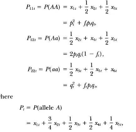
It follows from Table 1 that among adult mates in generation t,

1 1

2

2

PI,, = P(AA) = X]/

+

- x 9 1

+

- x31

=

p:

+

J5ptqt3 ( 1 )

1 1

Plz, = P(Au) = -

+

x41

+

-

2 2

where

P, = P(alle1e A)

q1 = 1 -

p,

and J measures the deviation of genotype

frequencies from those there would be with a Hardy- Weinberg structure.

The change in the frequency of A from one genera- tion of selection: It follows from Table l and Equations

1-3 that the genotype array of adults in generation

t

+

1 is equal to

2Ptqdl - J5) -

Therefore the frequency of A among these adults is

T

If selection is weak, we can neglect squares of s and

1

- 2hsp,qt(l

-fi)

- - ( S - 2hs)Dt

4

1

=

p,

+

sptqdp,

+

q&)

+

hsptqdl -

2Pt)

( 1 -

fi)

+

-

1 Dt[sqt -

M I

- 2pJI. (6)

4

Among random mating couples the frequency of A can be shown to remain

pR,+l.

In the special case in which heterozygotes are of intermediate viability so that h =

i,

Equation 6 reduces to

S 1

p,,+1

=

p,

+

2

Ptqt(1 -

J )

+

s

a . (7)

Now note that if there were no selection we would have

1 2

P,2,t+l = 2pt+1qr+1(1

-J+d

= 2P,qt(l -

J )

- - Dt 1

2

= P12t - - D,.

If there is selection,

pt+,

=

p ,

+

O ( s , sh), so that

P l 2 , t + l - P1et =

2P,qdJ

-

J + J

+

O ( s , sh)

1 2

=

-

- D,

+

O ( s , sh).

I shall henceforth assume that A is a rare allele, t is not large and

fo

is at least approximately equal to the equilibrium value F = @ / ( 4 - 3p) of the inbreeding coefficient as found by GHAI (1969). This means that we can neglect the last term on the right side of Equation 6 and replace Equation 6 by

P R t + l

=

p ,

+

p r q m

+

( 1 - F ) h s I . ( 8 )

We now consider couples for which the mates are full sibs. With weak selection the total number of such couples among adults of generation t

+

1 is propor- tional to

( 4

(:

8

4

4 l )

7

(

2 I )

1

TI =

s2

XI,

+

- %,

+

- X4,

16 1

)

+

sH(;

x 2 t

+

$

x4t)

1 1

+

- S X 4 ,

+

H 2 -

+'

+

X3,

+

-

X4,

+

- Xg,

+

4;

X4t

+

2

% t )

+

(&

x41

+

4

%t

+

%t 1

=

1

+

s 2x1,

+ .%+,

+

- x4,

f hS(x2t

+

2X3t

+

X4r

+

% t ) .

Hence, by Equations 1, 2 and 5

TI = 1

+

2

[ (

s

P:

+

Jptqt

+

4

Dt

l )

(

2

1

11

+

hs 2p,ql( 1 - J ) - - D,

=

T 2 .

If, for example, we have a couple of type AAxAa, its frequency of A is

i,

whereas for a couple of type A A X aa,

it is

i.

From these facts and Equations 1, 2, 4 and 5, it follows that the frequency

p , , + ,

of A among couples that are full sibs is approximately

' r ( l

T2

+ 2 r ) ( x , , + q x 2 , + - x 4 , 1 16 l ) + - ( 1 : + s + h s )

x

(;

x%

+

;

.,) +

;:

(1

+

s)xqt

+

- 1 ( 1

+

2hs)

2

(:

4 4

I

)

:

1

x

-

x2,

+

Xg,

+

- X 4 ,

+

-

X5,

+

- ( 1

+

hs)

x

($

X4t

+

2

Xh)} =

+

{*,

+

s(2P;

+

2 J p 4

2 8 1 )

(:

2

4

1

1

1 1

+ - D t - - E ,

+

hs - p r q t ( l - J ) - - D ,

+

1

E , ) }

=

h

{

p,

+

ptqt(

2sF

+ 2

3 hs( 1 -

4

1

+

- (2hs - s)E, ,

8

I

where

E' = x 2 1

+

x41 (9)

Now any particular mating type is generated by ran- dom mating with probability 1 - ,B and by full-sib mat- ing with probability

0.

Thus, if

p,,

hs and s are small, Equation 2 implies that

Et+, = (1 -

P )

[4($

+

Jptqt)p'q'(1 -

J )

+ 4p:qW

-

j J 2 I

+

P{

(;

x 2 t

+

1

X4')

c

4 1

11

[:

' I

4

1

+

- x 2 1

+

x 3 1

+

-

%+

4

%r

+

O(S, sh)

=

P

- E'

+

p t q t u - J ; ) -

2

a

+

O(S, sh,

p:)

=

- E t

P

+

Pptqt(l -

4.

(10) 2

If A is a favorable allele,

p,

is small and t is not large,

442 E. Pollak

There is thus a rapid convergence of Et to an approxi- mate equilibrium value

Therefore, the frequency of A among full-sib couples is, by Equation 11,

P,t+l

p,

+

sPtqt(2F - ( 1 - 4 )

4(2 -

P )

+

4(3 - P ) ( l - P)hsI =

pt

+ -

- ptqt

2 - P

X [Fs

+

(1 - F)hs]. (12)

This expression can also be shown to hold if h =

i,

in which case we do not have to solve for E.

Equations 8 and

12

together imply that the overall change in the frequency of A between adults of genera- tions t and t

+

l is

Equation 3 of CABALLERO and HILL (1992b), which was derived by using the theory of WRIGHT (1942), dif- fers from Equation 13 in that it does not contain the factor 2/

(2

-

P )

.

For partial selfing, this factor is indeed

missing, as shown by POLLAK and

SABRAN

(1992) for the special case where h =

y2.

W h y

then does it appear when there is partial full-sib mating?

The following is an explanation. Let z, and zj respec- tively, denote the frequencies of A in a male and a female that take part in a mating in a population with an equilibrium inbreeding coefficient F. Then, if

p,

is the frequency of A in generation t,

1 1

4

+

2P1qt(l

- r ; > * -

-

p;

= p t q , ( l

+

r ; > 7

and, following the reasoning of LI (1976),

Therefore the correlation between the frequencies of A in the mates is

2F

l + F

m = -

as found by WRIGHT (1921). In our case

Equation 13 may thus be rewritten as

Apt

=

plqt(Fs

+

(1 - F)hs)(l

+

m). (14)

Thus we see that because full sibs are more likely to have the same alleles than a random pair of individuals, a positive correlation between mates is induced in their frequencies of A. This results in a second increase within a generation in the frequency of A, which is m

times as large as that from viability selection.

An expression for the probability that a mutant sur-

vives: The standard expression in the literature for the change in the frequency of A with partial inbreeding was used by CABALLERO and HILL (199213) to derive an equation for the probability that A survives, given that it is initially present in only one heterozygote in a large population. This is

u =

2

- N e [Fs

+

(1 - F ) h s ] ,

N

where N and N, are, respectively, the population size and the effective population size. The latter was shown by CABALLERO and HILL (1992a) to be

4N

N, = (16)

2(1 - F )

+

&l

+

3 4 ’

where

02

is the variance of family size.

methods, that if s and hs are small,

POLLAK (1988) showed, by using branching process

and Yl, is the number of couples of type j among the progeny of a couple of type i. The types of couples, with subscripts in the same order as in the vectors and

p;,

are (1) A A X A A , (2) AAXAa, (3) AaXAa, (4)

A A X ;a and ( 5 ) AaX aa. It follows from Equation 17 and Equation A1 in the Appendix that if s and hs are small,

u = 2 - NP (1

+

m)[Fs

+

(1 - F ) h s ] (21) N

approximately.

DISCUSSION

If

p,

is very small and

qt

is near 1, Equation 13 can be written as

P , , l = 1 + - [Fs

+

(1 - F ) h s ] .

Pt

2 - P

In this form it is seen to be consistent with Expression

22 of POLLAK (1988) for p , which, roughly speaking, is the ratio of the number of copies of A in generation t

+

1 to that in generation t, if this allele is rare. Thus,

Apt

=

Ptqt(p - 1)

if

p,

is small and, by Equation 21,

u = 2 - N e ( p - l ) , N

where p - 1 is a measure of the selective advantage of A in comparison with a. If F = = 0 and hs is set equal to s’, Equation 22 reduces to

u = 2 - Ne s f ,

N

which is a result obtained by KIMURA (1964). The spe- cial case where N = N, was obtained by HALDANE (1927).

A simple special case of Ne is when there is a Poisson distribution of family size, but, as has been pointed out

by CABALLERO and HILL (1992b), the Poisson distribu-

tion of family size has to be defined carefully when there is partial inbreeding. If there are independent Poisson distributions of male and female offspring, a:

= 2. In this case

N(4 - 30) - N

N, =

2 ( 2

-

0 )

1

+

F

”

Alternatively, if the number of sib matings among off- spring of a couple has a Poisson distribution with mean and the number of random matings among them is an independent Poisson random variable with mean

2(1 -

p ) ,

then

a; = 4 p

+

2 ( 1

-

p)

= 2(1

+

p ) .

In this case Equation 16 reduces to

N ( 4 - 3P) N

N, = -

4 1

+

3 F ’

as found by POLLAK (1988).

I have assumed that t is small, as well as s and sh.

Thus,J should not deviate much fromfo

=

p/(4 - 3p)

for such values of t and, if not much time has passed since the allele A entered the population, its frequency would almost certainly remain low. Thus, the branching process approximation that describes the change in fre- quency of A should be satisfactory for small t, because it relies on A being rare enough that different matings with this allele at a particular time t generate indepen- dent lineages. Because, as pointed out by EWENS (1968),

the fate of a new mutant is largely determined while its frequency in the population is low, the approximation given by Equation 21 should be a good one under the aforementioned assumptions.

I am grateful to A. CABALLERO and three anonymous referees for helpful comments that led to the correction of some serious errors in an earlier version of this paper. This is journal paper no. 5-15406

of the Iowa Agriculture and Home Economics Experiment Station, Ames, Iowa, Projects 2588 and 3201.

LITERATURE CITED

CABALLERO, A,, and W. G. HILL, 1992a Effective size of nonrandom mating populations. Genetics 130: 909-916.

CABALLERO, A,, and W. G. HILL, 199213 Effects of partial inbreeding on fixation rates and variation of mutant genes. Genetics 131:

493-507.

EWENS, W. J., 1968 Some applications of multi-type branching pro- cesses in population genetics.J. Roy. Statist. Soc. Ser. B 30: 164-

175.

GHAI, G. L., 1969 Structure of populations under mixed random and sib mating. Theor. Appl. Genet. 39: 179-182.

HALDANE, J. B. S., 1927 A mathematical theory of natural and artifi- cial selection, Part V selection and mutation. Proc. Cambr. Philos. SOC. 23: 838-844.

KIMURA, M., 1964 Diffusion models in population genetics. J. Appl.

KIMURA, M., and T. OHTA, 1971 TheoreticalAspects ofPopulation Cmet-

ics. Princeton University Press, Princeton, NJ.

LI, C. C., 1976 First Course in Population G n e t i a . The Boxwood Press, Pacific Grove, CA.

POLLAK, E., 1988 On the theory of partially inbreeding finite popula- tions. 11. Partial sib mating. Genetics 120: 303-311.

POI.IAK, E., and M. SAHRAN, 1992 On the theory of partially inbreed- ing finite populations. 111. Fixation probabilities under partial selfing when heterozygotes are intermediate in viability. Genetics 131: 979-985.

Probab. 1: 177-232.

WRIGHT, S., 1921 Systems of mating, I-V. Genetics 6: 111-178. WRIGHT, S., 1942 Statistical genetics and evolution. Bull. A m . Math.

SOC. 48: 223-246.

444 E. Pollak

APPENDIX

As stated by POLM (1988),

X j

u o j ~ , = G i ~ o 5 , where

Gj is the number of gametes of type A contributed to offspring of a couple of type i when there is no selec- tion. Let G denote the total number of successful ga- metes contributed to offspring by one parental couple. Then G, has the same distribution as G, and because all offspring of matings of type 4 are heterozygotes, G4 is distributed as G/2. Thus Var

(E,

uojl$) =

d50:

and Var

( X j

uojcj) = d5&/4.

To obtain the distributions of GB, G3 and G5, we must define other random variables. First, let Gw and G,s be, respectively, the number of gametes of type A and the total number of gametes that a couple of type i contri- butes to sib mating couples among its progeny. Second,

GjR and GR will denote, respectively, the number of ga- metes of type A and the total number of gametes con- tributed by a couple of type i to its random mated progeny. Thus G = GS

+

G,, and, with neutral alleles,

E( Gs) = 4 0 and E( G,) = 4(1 -

p).

Let Bin(n,

p )

represent a binomial distribution with parameters n and

p.

Because of Mendelian segregation when only one of the mates in a couple is heterozygous, the conditional distributions of GPR, GZs, G5, and GSS,

given GK and G,s, are respectively

GnHl GR, G1,

-

G.

+

Bin

(-

GI2

I

)

2 2 ’ 2 ’

G2sI GK, Gs

-

Gs

+

Bin

(-

G~s

-)

1

2 2 ’ 2

’

G5RI G,, G~s

-

Bin

(?

-

-

,

3

:)

GSsl GR, Gs

-

Bin

(+,;).

Thus

Var

(x

uo,Y4j) = u&, E ~

i

{

FGR

:

“1

+

Var

[

i

( G,

+

G s ) ] ] =

&[

f

+

16

9

&]

and

Var

(x

uo,Ykj) =

d5

E ~

1

{

FGR

:

“1

+

Var

[VI}

=

d5[i

+

16

1 o:;]

.

Finally, if there is a couple of type 3, both mates are heterozygotes so that

G M GK, G.s

-

Bin

(

GK, -

1)

(

3

and

Gssl GR, Gs

-

Bin G,s, -

.

Hence

Var

(E

u o j ~ ; , ) = u& E ~

{

[

4

I

FGR;

7 1

GR

+

GS + Var

I

=

&[

1

+

4

1

“:I

.

It therefore follows from Equation 20 that

E

Po,

Var

(E

uojy;) = -

CC

pni&)d;

+

-

u&p03

1 1 16 i

1

4

x[-&+4+ 16 -

2op

+

5 7

P ( 1 -

P )

2

= u05 [4(4 Y 3 P )

+

4

-

3p 2(1 -

@)I

.

However, 1

+

3 F = 4/(4 - 30) and 1 - F = 4(1 -

p ) /

(4 - 3p). In addition, Gis equal to twice 12, the number

of offspring of a couple. Therefore

Z

pot Var

tC

UoIKj)

z 1

u05 N

-

” [a;(l

+

3E)

+

2 ( 1

-

a]

= u05 - . ( Al)

4 Ne

POLM (1988) derived a different expression from Equation A1 because of an erroneous assumption that