Simulation of Transitional Flow over an Elliptic Cone at Mach 8 using a One-Equation Transition/Turbulence Model

(1)

ABSTRACT

MALECHUK, ANDREW MARTIN. Simulation of Transitional Flow over an Elliptic Cone at Mach 8 using a One-Equation Transition/Turbulence Model. (Under the direction of Jack R. Edwards and Hassan A. Hassan.)

(2)

SIMULATION OF TRANSITIONAL FLOW OVER AN ELLIPTIC CONE AT MACH 8 USING A ONE-EQUATION TRANSITION/TURBULENCE MODEL

by

ANDREW MARTIN MALECHUK

A thesis submitted to the Graduate Faculty of North Carolina State University

in partial fulfillment of the requirements for the Degree of

Master of Science

AEROSPACE ENGINEERING

Raleigh 2002 APPROVED BY:

_________________________ _________________________ Dr. Jack R. Edwards Dr. Hassan A. Hassan

(3)

BIOGRAPHY

ANDREW MARTIN MALECHUK

75 N Fawn Forest LN Campus Box 7910

Pittsboro, NC 27312 NCSU

(919) 545-0869 Raleigh, NC 27695

[email protected] (919) 515-5250

EDUCATION

Masters Aerospace Engineering.

(Computational Fluid Dynamics Concentration). Minor Mathematics.

North Carolina State University, Raleigh NC. GPA - 3.5.

Thesis: Simulation of Transitional Flow over an Elliptic Cone at Mach 8 using a One-Equation Transition/Turbulence Model. B.S. Aerospace Engineering.

North Carolina State University, Raleigh NC. Overall GPA - 3.6, Major GPA - 3.6.

Graduation Date - May 2000.

RELEVANT COURSES

• Computational Fluid Dynamics. • Aircraft Design.

• Computational Reactive/2-Phase Flows. • Incompressible Aerodynamics.

• Advanced Compressible Aerodynamics. • Boundary Layer Theory.

• Numerical Analysis.

• Incompressible and Compressible Flow Labs.

IMPORTANT PAPERS

Sandia National Laboratories Summer 2001 Internship

• Implementation of the NCSU Transition Model into the SACCARA Compressible Fluid Mechanics Code.

(4)

BIOGRAPHY (continued) WORK

EXPERIENCE

8/00-11/02 NC State University Research Assistant - Raleigh, NC

• Modified existing parallel computational fluid dynamics code to include NCSU one-equation transition/turbulence model.

• Examined effects of various parameters on location and extent of flow transition using hypersonic 3-D cone and modified code.

• Lectured Aerospace Engineering classes.

6/01-8/01 Sandia National Laboratories Intern - Albuquerque, NM 5/02-8/02

• Added NCSU transition/turbulence model to SACCARA CFD code. • Obtained L Security Clearance while working in department 9115.

• Presented internship work at SNL symposium receiving 94 out of 100 possible grade points.

6/99-1/00 CargoLifter Inc. Intern - Raleigh, NC • Researched effects of inclement weather on airships. • Created airship database/library.

• Performed market studies.

SOCIAL

Activities

• Senior Aircraft Design Team Leader.

• Supervisor of annual special needs children’s beach retreat. • Ground crew for annual Winston-Salem, NC air show. • Encounter College Retreat leader and coordinator. • NC State Intramurals.

Awards

• 8 Semesters on Dean’s List.

• Sigma Gamma Tau Honor Society Member.

COMPUTER EXPERIENCE

• Systems – UNIX, LINUX.

• Software – Microsoft Office, ANSYS, Tecplot, Word Perfect, MATLAB, MAPLE, Pro Engineer, AutoCAD.

• Programming Languages – FORTRAN (MPI).

(5)

ACKNOWLEDGEMENTS

(6)

TABLE OF CONTENTS

LIST OF TABLES... vi

LIST OF FIGURES ... vii

NOMENCLATURE ... ix

1 INTRODUCTION ... 1

1.1 Importance of Modeling Transition ... 1

1.2 Previous Research... 1

1.3 Objectives of Research ... 4

2 MODEL DESCRIPTION ... 5

2.1 Introduction... 5

2.2 Eddy Viscosity-Transport Equation for Non-Turbulent Fluctuations ... 6

2.3 Spalart-Allmaras Turbulence Model... 8

2.4 Transition Region Modeling... 9

2.5 Transition Criteria... 11

2.6 Complete Transition/Turbulence Model... 12

2.7 Calculation of Eddy Viscosity ... 13

3 CALCULATION DETAILS ... 13

3.1 Elliptic Cone Grid... 13

3.2 Determining Boundary Layer Edge Value ... 14

3.3 Code Description and Boundary Conditions ... 17

3.4 Initialization and Run Parameters... 17

4 RESULTS AND DISCUSSION... 18

4.1 Experimental Data ... 18

4.2 Calculation of Heat Flux... 19

4.3 Convergence ... 19

4.4 Fully Laminar and Turbulent Flow... 20

4.5 Transitional Region... 21

4.6 Comparison of Methods... 22

5 CONCLUSIONS... 25

5.1 Conclusions... 25

LIST OF REFERENCES... 28

APPENDIX... 29

TABLES ... 30

FIGURES... 31

(7)

LIST OF TABLES

Table 1: Freestream properties for simulations ... 30 Table 2: Transition location and magnitude with

(8)

LIST OF FIGURES

Figure 1: Elliptic cone grid orientation... 31 Figure 2: Velocity distribution, X=0.04m, θ =61.7o

(Re/L=1.98x106/ft, transitional)... 31 Figure 3: Pressure distribution, X=0.04m, θ =61.7o

(Re/L=1.98x106/ft, transitional)... 32 Figure 4: Momentum distribution, X=0.04m,

=

θ 61.7o_{(Re/L=1.98x10}6_{/ft, transitional)... 32}

Figure 5: Convergence history (Re/L=1.98x106/ft,

fully laminar and turbulent) ... 33 Figure 6: Turbulent residual norm history

(Re/L=1.98x106/ft, transitional)... 33 Figure 7: Turbulent residual norm history

(Re/L=6.09x105/ft, transitional)... 35 Figure 10: Pressure distribution X=0.933m

(Re/L=1.98x106/ft, fully laminar)... 35 Figure 11: Temperature distribution X=0.933m

(Re/L=1.98x106/ft, fully laminar)... 36 Figure 12: Temperature distribution X=0.933m

(Re/L=1.98x106/ft, fully turbulent)... 36 Figure 13: Heat flux distribution along rays of cone

(Re/L=1.98x106/ft, fully laminar)... 37 Figure 14: Heat flux distribution along rays of cone

(Re/L=1.98x106/ft, fully turbulent)... 37 Figure 15: Transition criteria over elliptic cone

(Re/L=1.98x106/ft, Tu=1.575) ... 38 Figure 16: Intermittency function over elliptic cone

(Re/L=1.98x106/ft, transition, Tu=1.575) ... 38 Figure 17: Viscosity distribution θ=63o

(Re/L=1.98x106/ft, transitional, Tu=1.575) ... 39 Figure 18: Non-turbulent time scale X=0.060m

(Re/L=1.98x106/ft, transitional)... 39 Figure 19: Heat flux distribution along rays of cone

(Re/L=1.98x106_{/ft, ISDE,}_Tu_{=1.5) ... 40}

Figure 20: Heat flux distribution along rays of cone

(Re/L=1.98x106/ft, BLES, Tu=1.5) ... 40 Figure 21: Heat flux distribution along rays of cone

(Re/L=1.98x106/ft, BLES, Tu=1.575) ... 41 Figure 22: Heat flux distribution along ray of cone

(Re/L=1.98x106/ft, θ=450, Tu=1.575) ... 41

(9)

LIST OF FIGURES (continued) Figure 23: Heat flux distribution along rays of cone

(Re/L=1.03x106, ISDE, Tu=1.5)... 42 Figure 24: Heat flux distribution along rays of cone

(Re/L=1.03x106_{/ft, BLES,}_Tu_{=1.575) ... 43}

(Re/L=7.8x105/ft, ISDE, Tu=1.5) ... 43 Figure 27: Heat flux distribution along rays of cone

(Re/L=6.09x105/ft, ISDE, Tu=1.5) ... 45 Figure 30: Heat flux distribution along rays of cone

(Re/L=6.09x105_{/ft, BLES,}_Tu_{=1.5) ... 45}

(10)

NOMENCLATURE

a = non-turbulent fluctuation constant (first-mode)

b = non-turbulent fluctuation constant (second mode)

Cb1 = Spalart-Allmaras model constant (0.1355) Cb2 = Spalart-Allmaras model constant (0.622) Cp = specific heat coefficient

Ct = model constant (0.35)

Ct3 = Spalart-Allmaras model constant (1.2) Ct4 = Spalart-Allmaras model constant (0.5) Cw1 = Spalart-Allmaras model constant (3.239)

Cµ = model constant (0.09)

c1 = model constant (0.00004) c2 = model constant

c3 = model constant (0.00002) c4 = model constant (0.15) c5 = model constant (0.0001) d = distance to nearest wall

ft2 = turbulence function in Spalart-Allmaras model fv1 = wall damping function in Spalart-Allmaras model fw = wall blockage function in Spalart-Allmaras model k = non-turbulent fluctuation energy

n = normal vector

Pr = Prandtl number (0.72)

(11)

NOMENCLATURE (continued)

p = pressure

qw = wall heat flux

Re = Reynolds number

RT = transition criteria function S = rotation tensor

s = surface distance

sT = surface distance to transition location Tu = average free-stream fluctuation intensity

T = temperature

t = time

U = total velocity

u = x-axis velocity

δ*_{= displacement}_thickness

Γ = intermittency function

κ = von Karman constant (0.41)

µ = viscosity

ν = kinematic viscosity

νnt = non-turbulent eddy viscosity

νt = eddy viscosity

v_% = transported eddy viscosity in Spalart-Allmaras model Ω = rotation tensor magnitude

(12)

NOMENCLATURE (continued)

ρ = density

σ = model constant (0.666667)

σl = diffusion term function based on flow regime

σt = diffusion term function based on flow regime

τ = non-turbulent time scale

Subscripts

l = laminar

1 = first-mode 2 = second-mode

e = boundary layer edge

HIDE = high disturbance environment

j = tensor notation index

k = kinetic energy

l = laminar

max = maximum

min = minimum

nt = non-turbulent

T = transitional

t = turbulent

w = wall

∞ = freestream

(13)

NOMENCLATURE (continued) Superscripts

* = boundary layer reference state ~ = working variable

(14)

1 INTRODUCTION

1.1 Importance of Modeling Transition

Since the early days of aero-sciences it has been known that two regimes of fluid flow exist: laminar and turbulent. In many real world situations though, both conditions exist simultaneously, with a fluid flow transitioning from laminar to turbulent somewhere along the length of an object in the flow. The location of transition onset is extremely important in the design and analysis of hypersonic vehicles since many important parameters are dependent upon whether the conditions are transitional, laminar or turbulent. Specifically, experimental data has shown that skin friction and heat transfer tend to be larger in the turbulent region than in the laminar region. Peak values of skin friction and heat transfer may, however, occur within the transitional region. Therefore it is important not only to locate the points at which transition onset takes place but also to determine the spatial extent over which transition to turbulence occurs. With these facts in mind, the importance of correctly predicting the transition location and extent in a particular flowfield is apparent. Therefore, it should be no surprise that development of a computational fluid dynamics (CFD) model that accurately predicts transitional flows is held to be one of the most important goals of the CFD discipline.

1.2 Previous Research

(15)

Hassan [1]. This was done through the combination of a kinetic energy (k) and enstrophy (ζ) turbulence model with a model for the growth of laminar fluctuations. Using the

minimum skin friction or heat transfer as the location of transition (due to the correlation of these properties and transition onset location as stated in Section 1.1) was found to be limited to simple shapes and the absence of adverse pressure gradients. The research determined that the transition onset location along the test body is more accurately determined for a wider range of environments by determining the point at which the ratio of turbulent and non-turbulent kinematic viscosities as shown in Equation (1.1) first exceeds unity when moving downstream from the front of the geometry.

v C

v R_T

µ ~

= (1.1)

Dhawan and Narasimha’s intermittency expression [2] was used to mix the non-turbulent and turbulent model characteristics in the transitional region of the flow. This model was then extended to second-mode disturbances be McDaniel, Nance, and Hassan [3]. One weakness of the model is that the derived first-mode and second-mode timescales (Equations (1.2) and (1.3)), which drive the growth of laminar fluctuations are based on a curve fit using the average turbulence intensity, Tu, of the flow:

1 1

2

/

0.069( 0.138) 0.00819

a

a Tu

τ = ω

= − + _(1.2)

2 b/ 2

τ = ω (1.3)

This curve fit is only accurate for Tu less than or equal to 0.5, limiting the model’s use to low disturbance-environment conditions.

Using knowledge gained from the two-dimensional simulations, the k-ζ

(16)

attempt to define the disturbance mode that bypassed the first and second-modes and to extend the model to three-dimensions. The result was the definition of a high disturbance environment (HIDE) mode that was found to dominate the other modes of transitional flow for high Mach numbers and larger values of Tu. The average turbulence intensity is still used to define the laminar fluctuation time scale that drives the non-turbulent fluctuation model, but the time scale is also dependent upon the local Reynolds number and boundary layer characteristics:

2 * 1

1/8 2

Re

2 0.9448

c HIDE

e

c U

c T

δ

u ν

τ =

= ×

(1.4)

The boundary layer edge values for the calculation of the Reynolds number and displacement thickness were found by extracting and saving surface flow parameters along the test subject from a converged inviscid run with the code. An elliptic cone with aspect ratio of 2:1 at Mach 8 with Tu=1.5 was used as the test case with matching experimental data provided by Kimmel, Poggie, and Schwoerke [5]. A minimum heat transfer criteria was used around the circumference of the cone to define the transition onset location. Only one quarter of the cone flowfield was simulated because of the bilateral symmetry of the geometry. When compared with experimental heat transfer data for three rays along the cone (0o, 45o, and 88o) over a variety of Reynolds numbers, the modified model performed well at predicting not only the transition onset location, but also the spatial extent over which transition occurred.

With the success of the k-ζ transition/turbulence model having been established,

Edwards, Roy, Blottner, and Hassan [6] proceeded to develop a one-equation transition/turbulence model based on combining an eddy viscosity-transport model for

(17)

non-turbulent fluctuation growth with the Spalart-Allmaras turbulence model. Since the Spalart-Allmaras model is a single equation, is relatively insensitive to normal grid spacing at the wall, and produces a good mixture of accuracy and robustness for wall-bounded turbulent flows, it is a very desirable model to use in a transition/turbulence model. Since most of the initial test cases involved turbulence intensities less than 0.5, a curve fit similar to that used in Warren and Hassan [1] was once again used to define the laminar time scale:

03 . 0

) ( 05050 . 0 ) ( 001801 .

0 009863 .

0

/

2 1

=

+ −

=

Tu

Tu Tu

a

a ϖ

τ

(1.5)

The criterion for transition in Equation (1.1) was used to determine the location of transition onset in the flowfield. The model was applied with reasonable success to transitional flows over a flat plate, a supercritical airfoil, a multi-element airfoil in landing configuration, a circular cylinder, and a sharp cone, all of which are two-dimensional or axisymmetric flows. The predictions were found to be very similar to

those obtained using the k-ζ transition/turbulence model. The success of this research produced the desire to examine the effectiveness of the Spalart-Allmaras transition/turbulence model in a hypersonic, three-dimensional, high turbulence intensity environment.

1.3 Objectives of Research

Past research has resulted in the development of reasonably accurate transition/turbulence models based on the k-ζ and Spalart-Allmaras turbulence models.

(18)

three-dimensional flows with high average turbulence intensities. This involves the modification of the non-turbulent component of the model to include a time scale characteristic of high disturbance environment fluctuation growth in a manner similar to

that used in the three-dimensional version of the k-ζ transition/turbulence model. The test

case for this research is again flow over an elliptic cone with aspect ratio of 2:1 at Mach 8 with Tu=1.5. This case is useful in that it contains heat flux measurements across a wide range of Reynolds numbers [5]. Comparisons with this data will provide a first assessment of the effectiveness and accuracy of the extended one-equation model.

2 MODEL DESCRIPTION 2.1 Introduction

In an effort to preserve the structure of the earlier model, as much of the two-dimensional Spalart-Allmaras transition/turbulence model as is possible is left unmodified and is transferred directly to the three-dimensional, high average turbulence intensity model. The major modifications involved in the conversion of the model involve the redefinition of the eddy viscosity-transport equation in the non-turbulent region of the flow to account for HIDE-driven transition. Since the three-dimensional HIDE version of the k-ζ transition/turbulence model [4] provides reasonably accurate

results, its model for non-turbulent fluctuation growth is transformed into an eddy viscosity-transport equation in a manner identical to that employed in Reference [6]. This model is then combined with the Spalart-Allmaras model to yield an approach designed to predict the characteristics of transitional, three-dimensional, high-speed flows under high disturbance environment conditions.

(19)

2.2 Eddy Viscosity-Transport Equation for Non-Turbulent Fluctuations

The framework for the eddy viscosity-transport equation for non-turbulent fluctuation growth is taken from the successful HIDE model [4]. The keys to transforming the model into a usable form for combination with the Spalart-Allmaras one-equation transition/turbulence model are as follows: First, the eddy viscosity definition and non-turbulent energy fluctuation energy equation are presented in Equations (2.1) and (2.2).

nt nt

v =C kµ τ (2.1)

2 _1.8

3

nt nt

k j j

Dk k v k

v

Dt τ x v x

 

∂   ∂

= Ω − +_∂  + _∂ 

 

 

  (2.2)

The next step is to multiply both sides of Equation (2.2) by C_µτ_nt.

2 _1.8

3

nt nt nt nt nt

k j

Dk k v k

C C v v C

Dt x x

µτ µτ _τ µτ

j

 

  ∂   ∂

=  Ω − +_∂ _ + _ _∂ 

 

    (2.3)

The relationship in Equation (2.1) can now be used to convert Equation (2.3) into a transport equation for an eddy viscosity characteristic of non-turbulent fluctuations.

2 _1.8

3

nt nt nt

nt nt nt

k j j

Dv v v v

C v v

Dt µτ τ x x

 _∂ 

∂  

= Ω − +_∂  + _∂ 

 

 

  (2.4)

It should be noted that the form for the diffusion term is not exact. Rather, it is assumed

that spatial variations of τ_nt are small enough so that the C_µτ_nt term may be brought

(20)

5

3 4

,

3 4 5

1

0.00002, 0.15, 0.001

nt

k HIDE

v c

c c S

v

c c c

τ   =_ + Γ_ +   = = = k

v (2.5)

The term in Equation (2.5) is Dhawan and Narasimha’s intermittency expression [2], which is discussed more thoroughly in the description of the transitional region of the model in Section 2.4.

Γ

For simplicity the norm of the strain rate tensor, S, in Equation (2.5) is approximated in Equation (2.6), where Ω is the vorticity magnitude.

2

Ω ≈

S (2.6)

Equation (2.6) can then be inserted into (2.5) with the result shown in Equation (2.7).

5 3 4 , 1 2 nt k HIDE v c c v v τ Ω   =_ + Γ_ +   c k (2.7)

The kinetic energy term in Equation (2.7) is removed by solving for k in Equation (2.1) and substituting this expression into Equation (2.7):

5 3 4 , 1 2 nt nt

k HIDE nt

v

c c

v v _µ

c v C τ τ Ω   =_ + Γ_ +

  (2.8)

This result can now be placed into Equation (2.4) to complete the equation for the non-turbulent part of the one-equation transition/turbulence model:

        ∂ ∂       + ∂ ∂ +         + Ω       ₊ _Γ − Ω = j nt nt j nt nt nt nt nt nt nt x v v v x vC v c c v v c v v C Dt Dv 8 . 1 3 2 5 4 3 2 τ τ µ µ (2.9)

The final piece of the non-turbulent section of the model is the formulation of the laminar

time scale, τ_nt_,_HIDE. The form for this term is taken from Reference [4] and is shown in

Equation (2.10)

(21)

2 * , 1 1 1 8 2 Re 0.00004 2 0.9448 c

nt HIDE c

c

c T

δ

τ =

=

= × u

(2.10)

The values defining the Reynolds number in (2.10) come from 99% of the boundary layer edge values under any resulting shock produced by the body in the flow. There is more than one method to extract these edge values from the flowfield, and two of these are

discussed thoroughly in Section 3.2. The displacement thickness, _δ*_{, in Equation (2.10)}

is defined in (2.11).

n d U u e e r

∫

      − = δ ρ ρ δ 0

* ₁ _(2.11)

In Equation (2.11), nv is the normal distance from the surface and δ is the edge of the boundary layer under any resulting shock.

2.3 Spalart-Allmaras Turbulence Model

The Spalart-Allmaras turbulence model used in the creation of the one-equation transition/turbulence model is based on the paper by Spalart and Allmaras [7] and is shown for completeness in the Appendix.

(

)

(

)

2 2

2 2 21 1 2 1 ~ ~ ~ 1 ~ ~ ~ 1 ~         ∂ ∂ +         ∂ ∂ + ∂ ∂ +             ₋ − Ω − = j b j j t b w w t b x v C x v v v x d v f C f C v f C Dt v D σ σ κ (2.12)

(22)

kinematic viscosities is expected to be large enough once the flowfield is entirely turbulent so that the f_t₂ function in Equation (2.13) can be considered zero.

0

2 4

~

3

2 = =

              − v v C t t t e C

f (2.13)

This reduces the production and destruction terms of the Spalart-Allmaras turbulence model to Equation (2.14), which is used for the turbulent region of the one-equation transition/turbulence model.

(

)

2 2

2 1 1 ~ ~ ~ 1 ~ ~ ~ ~         ∂ ∂ +         ∂ ∂ + ∂ ∂ +       − Ω = j b j j w w b x v C x v v v x d v f C v C Dt v D σ

σ (2.14)

2.4 Transition Region Modeling

The transition region of the flow is modeled by using a weighted average of the non-turbulent and turbulent eddy viscosity equations through the use of Dhawan and Narasimha’s intermittency expression [2], modified as shown in Equation (2.15).

( )

(

)

( ) 2 0.412 0.75 , 1 max ,0

Re 9.0 Re

T T s s e s s ζ λ θ θ θ θ ζ λ − Γ = − − = = (2.15)

The transition location, s_T

( )

θ , is the distance from the stagnation point on the body to

the surface circumferential location of the start of the transition region as dictated by the transition criteria stated in Section 2.5. Also, s is the surface distance from the stagnation point to any point on the surface of the body. The Reynolds number calculations are defined by 99% of the boundary layer edge values. At surface distances less than the transition location, the intermittency function returns a value of zero, while at surface

(23)

distances far enough from the transition onset location, the function returns a value asymptotically approaching one. In between the transition location and this trailing point, the function returns a monotonically increasing value between zero and one, connecting both of the extremes. Through this process, the transitional region of the final one-equation transition/turbulence model is defined by using the intermittency function to provide a weighted mix of the non-turbulent and turbulent components of the model based on the location along the surface of the test body (See Section 2.6).

Examining Sections 2.2 and 2.3, it is apparent that the diffusion terms in both the non-turbulent and turbulent sections of the model resemble one another. The intermittency function can therefore be used to combine the two components into one single term (2.16).

2 2

1 1 _b

j l t j j

C

v v

x σ σ ν x σ x

   Γ 

∂ ₊ ∂ ₊

 

   _ _

∂ __ _∂ _

 ∂ ∂

  

% %



% _(2.16)

where

(

)

1 1

3 1

1.8 1

l

t

σ σ

Γ − Γ = + Γ

= + − Γ

(2.17)

Looking at (2.16) and (2.17), it can be seen that when Γ returns a value of 0 (the turbulent region of the flow), the diffusion terms in the equation return to the non-turbulent form found in Equation (2.4), and when Γ returns a value of 1 (the turbulent region of the flow), the diffusion terms in the equation return to the turbulent form of Equation (2.12). When returns values between zero and one, a weighted average of the diffusion terms is achieved.

(24)

It was discovered in earlier research [6] that an extra term is required in the transitional region to more accurately model the rise in wall shear stress, or wall heat transfer, that occurs just downstream of transition onset. The result is the term found in Equation (2.18), which is added as an additional production term for the eddy viscosity.

(

1

)

t

CΓ − Γ Ωv_% (2.18)

The constant is set to 0.35, following Reference [6]. Examining the equation, it can be

seen that (2.18) is active only in the transitional region (0<

t

C

Γ<1).

2.5 Transition Criteria

The criterion for transition of the flow from laminar to turbulent was borrowed from past research work [1] and is based on a ratio of turbulent and non-turbulent kinematic viscosities (2.19).

T

v R

C vµ

= % (2.19)

Transition onset is determined by first calculating the maximum value of RT in a

boundary layer profile along each axial station over each circumferential ray. Next, a search from the stagnation point aft is done to find the first axial location along each circumferential ray at which the maximum value of RT first exceeds unity. Once this

point is found, it is designated the transition onset location, s_T

( )

θ , along that ray. If the

value of 1.0 in Equation (2.19) is never exceeded along a ray, then the flow is considered laminar over the entire ray, with a value of zero being returned from the intermittency function along the entire ray.

(25)

2.6 Complete Transition/Turbulence Model

Now that they are established, all of the separate pieces of the one-equation transition/turbulence model can be combined into Equations (2.20) and (2.21) through the use of the intermittency function [2] in Equation (2.15).

(

)

(

)

        ∂ ∂       + ∂ ∂ +         ∂ ∂ Γ +               − Ω Γ + Ω Γ − Γ +                 + Ω       ₊ _Γ − Ω Γ − = j t l j j b w w b t nt nt nt nt nt nt x v v x x v C d v f C v C v C vC v c c v v c v v C Dt v D ~ ~ 1 1 ~ ~ ~ ~ ~ 1 2 1 ~ 2 2 2 1 1 5 4 3 2 σ σ σ τ τ µ µ (2.20) where

(

)

1 1 3 1 1.8 1 l t σ σ σ σ Γ − Γ = + Γ = + − Γ (2.21)

(26)

2.7 Calculation of Eddy Viscosity

Given the transported quantity v~ as obtained from Equation (2.20), the eddy viscosity as given in Reference [6] is presented in Equation (2.22).

(

1

)

1 1

t v

v =v_%_ + Γ f − _ (2.22)

1 t

v =vf_% _v (2.23)

When the intermittency function returns a value of unity (i.e. turbulent flow) Equation (2.22) returns to the purely turbulent Spalart-Allmaras form in Equation (2.23).

3 CALCULATION DETAILS 3.1 Elliptic Cone Grid

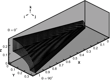
The experimental test case simulated in this research is Mach 8 flow over an elliptic cone [5]. This case was used in Reference [4] in the study of HIDE-driven transition using the k-ζ transition/turbulence model. The boundaries for the elliptic cone

grid are shown in Figure 1 and are based on a sharp-nosed cone with an elliptical cross section of aspect ratio 2:1, and a length of 40 inches (1.016 m). The cone half-angle is 7o

along the minor axis. Since the cone is modeled at 0o angle of attack, the bilateral symmetry of the flowfield requires only one quadrant of the flow to be simulated. Using a cylindrical coordinate system, θ =0o corresponds to the top centerline, or minor axis endpoint, while θ=90o corresponds to the leading edge or major axis endpoint. , The grid contains 129 grid points in the i-direction (axial coordinate), 65 points in the j-direction (circumferential coordinate), and 73 points in the k-direction (radial coordinate). The distance between the outer radial boundary (k=73) and the surface (k=1) was chosen to be large enough so that the grid contains the resulting conical shock, and the flow

(27)

properties along the k=73 boundary are close to freestream conditions. The grid nodes are tightly packed against the surface of the cone, and the spacing between nodes becomes greater as the distance from the surface increases. This is done to capture the boundary layer characteristics around the model more precisely.

3.2 Determining Boundary Layer Edge Value

To determine boundary layer edge properties for use in the equations found in Section 2, an accurate way of determining the boundary layer edge is first required. For flowfields where shockwaves are not present, the edge of the boundary layer is usually considered to be located at a distance where the local velocity reaches approximately 99% of its freestream value. When shockwaves are present, such techniques are no longer valid due to the discontinuous change in fluid properties across the shock. A conical shock develops in the flowfield discussed in this paper, so a technique had to be devised in order to define the boundary layer edge values.

(28)

Therefore, it was determined that a new approach was needed to effectively locate the boundary layer edge, and ultimately, the fluid property values at this location.

Profile data from the purely laminar region was extracted from the initial runs of the transition/turbulence code in an effort to search for a better way to locate the boundary layer edge. The u-velocity profile in Figure 2 shows the boundary layer growth, and the conical shock is noticeable. Since the boundary layer edge exists under the conical shock, the pressure profile was then examined in Figure 3 to explore the possibility of locating the edge of the shock as a limit for the search for the boundary layer edge. Even though the grid is not very refined around the conical shock, the discontinuity in the pressure profile is still evident. A search was added to the code to locate the largest pressure gradient along every radial grid line emanating from the cone surface. This point corresponds to the conical shock location. Test cases were run using nodes a set distance (from zero to 4 grid nodes depending on the run) below the shock as the boundary layer edge, but a new problem was detected dealing with the calculation of

the displacement thickness, _δ*_{. As the code was progressing towards convergence,}

negative time scales would start to develop, causing the code to become unstable. Looking at the definition of the time scale in Equation (3.1) and knowing that the flow properties such as velocity were being returned as positive values, the displacement thickness was labeled as the problem.

2 *

, 1Re

c

nt HIDE c δ

τ = (3.1)

Equation (3.2) shows the calculation of the displacement thickness and its dependence on the edge values of velocity and density.

(29)

n d U

u

e e

r

∫



  

 

−

= δ

ρ ρ δ

0

* ₁ _(3.2)

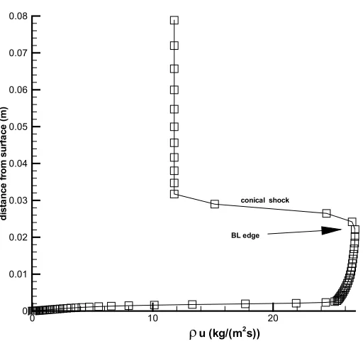
In a situation where the multiplication of the established edge values of velocity and density are lower than the local product of velocity and density, this part of the integral calculation would yield a negative value. If there is enough of a difference between the two values, the overall integral would return a non-positive value. Checks were performed and it was determined that the axial-momentum (ρu) profile grew in

magnitude with increasing distance from the surface in a manner similar to the velocity profile in Figure 2, but tended to decrease as the flow approached the conical shock as is shown in Figure 4. It was noticed that the maximum value of the axial-momentum profile occurred close to, but slightly under, the conical shock location. This information was used to define the edge of the boundary layer, and ultimately the boundary layer edge values.

(30)

3.3 Code Description and Boundary Conditions

REACTMB [8], an implicit, parallel code for solving general reactive flow problems, was used to perform all runs for this research. The grid was decomposed into 64 equivalent blocks shown in Figure 1 and mapped to 64 processors of the NCSC IBM SP2 in an effort to reduce the amount of real-world clock time required to achieve convergence. Due to the parallelism of the code, it is necessary to send local boundary layer data to a master processor, which then performs a global search to determine the transition onset locations (See Section 2.5). The resulting intermittency function is then passed to the other processors. Freestream values are enforced along the incoming flow boundary, surface conditions (no-slip and adiabatic wall) are enforced along the surface, fluid properties are extrapolated at the imax and kmax planes, and symmetry conditions are

enforced along the jmin and jmax planes.

3.4 Initialization and Run Parameters

Before each run, the entire domain (with the exception of the solid walls) is set to freestream conditions to initiate each run based on the inputted Reynolds number per meter, freestream temperature (K), and freestream Mach number. As per Reference [6],

the freestream value of the transported quantity is chosen to be 0.0001 . The code is

typically run for 4,000 iterations to achieve a steady-state solution. The CFL number is ramped from 0.5 to 10.0 over the course of the run. Flows at four different Reynolds numbers (See Table 1) were simulated to cover the range of transitional data that was compiled experimentally [5] and to help determine the accuracy of the model for a variety of flow conditions. In previous research [4], the average turbulent intensity, Tu, in

v_% v_∞

(31)

the tunnel during the tests with the elliptic cone was chosen to be 1.5. Therefore, c2=1.988 in the non-turbulent time scale of Equation (3.3):

2 *

, 1

1

1 8 2

Re 0.00004 2 0.9448

c

nt HIDE c

c

c T

δ

τ =

=

= × u

(3.3)

Reference [4] chooses this value as 2.0, so in an effort to determine the model’s sensitivity to Tu, a set of runs was performed with Tu=1.575, which sets c2=2.

Fourteen runs were performed. A purely laminar case and a purely turbulent case with a Reynolds number of 1.98x106/ft were simulated to compare with transitional runs to ensure that values before and after the transitional region matched the corresponding purely laminar and turbulent solutions. All four studied Reynolds numbers were then run using the ISDE method to define boundary layer edge values along with Tu=1.5. Next, all four Reynolds numbers were simulated using the BLES method described in Section 3.2 along with Tu=1.5 to compare the different methods of defining the boundary layer edge values. Lastly, all four Reynolds numbers were simulated using the BLES method and Tu=1.575 using the value in Reference [4] for the c2 constant in order to determine

the sensitivity of the model to the choice of Tu.

4 RESULTS AND DISCUSSION 4.1 Experimental Data

The experimental data for these runs is obtained from Reference [5]. Transitional data, specifically heat flux at the wall, qw,, was recorded over a wide variety of Reynolds

(32)

Schmidt-Boelter gauges. These gauges have an uncertainty of ±10% in two-dimensional

flows with greater uncertainty in three-dimensional flows. Data was recorded along the 0o, 45o, and 88o circumference locations on the quadrant of the elliptic cone.

4.2 Calculation of Heat Flux

In the results that follow, computed heat fluxes along the cone surface are compared with experimental data. The heat flux at the surface of the cone is calculated using Equation (4.1) along the rays that correspond to the circumferential locations where experimental data was recorded.

avg p w

w r

C T

q

P n

µ ∂

=

∂r (4.1)

This computational data can then be plotted along with the experimental heat flux to examine how well the model predicts the transition onset location, extent, and magnitude with respect to the heat flux.

4.3 Convergence

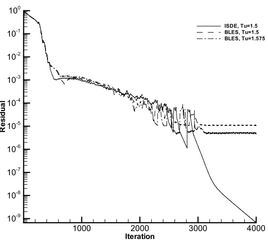
As was discussed in Section 3.4, all runs were performed for 4,000 iterations as this converged the turbulence norm to a leveling point. The norm convergence history is shown for the fully laminar and fully turbulent simulations in Figure 5. The turbulent run converges in approximately 1,200 iterations while the laminar run takes the full 4,000 iterations to reach the same level of convergence. Both runs reach their converged state in a rather linear fashion. The turbulent residual norm is shown in Figure 6 for the Re/L=1.98x106/ft transitional runs. The ISDE method converges four orders of magnitude beyond the point where the BLES methods level off. Unlike the linear trends found in the laminar and turbulent convergence curves, the convergence curves for this transitional Reynolds number are jagged and oscillatory. As the transition/turbulence

(33)

model equations proceed towards an equilibrium, or converged state, grid points near the transition onset locations may shift from non-turbulent to transitional, causing the equation system to relax towards this new equilibrium state. This point movement eventually ceases once the solution reaches its steady state. Figure 7 plots the turbulence norm history for transitional runs with Re/L=1.03x106/ft. This time, the BLES method converges two orders of magnitude faster than the ISDE technique. As with the Re/L=1.98x106/ft case, spikes in the convergence history occur. The transitional simulations with Re/L=7.8x105/ft are shown in Figure 8. The BLES technique converges five orders of magnitude further than the other technique, and peaks in the curves once again occur. Lastly, Figure 9 shows the turbulence residual norm history with Re/L=6.09x105/ft. The convergence comparison cannot be assessed accurately because the ISDE technique reaches the 4,000 iteration stopping criteria before completely converging. The jagged portions of the convergence curves evident in the other three Reynolds numbers are not as prominent in this set of simulations. This is related to the small region of transitional flow located on the cone (i.e. the majority of the cone is in a purely non-turbulent state).

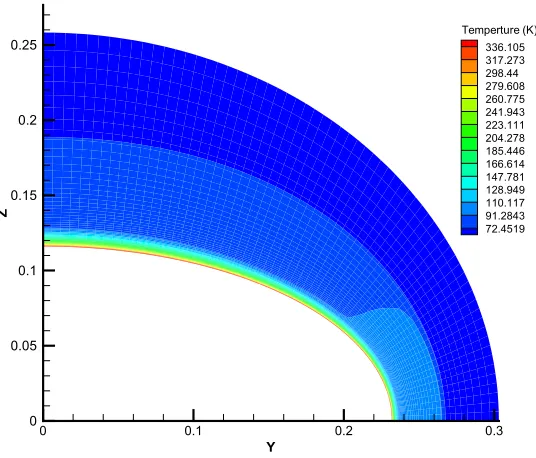
4.4 Fully Laminar and Turbulent Flow

(34)

plot at the same cross section is shown in Figure 11 revealing a thicker thermal boundary layer for the turbulent simulation. Computed heat flux distributions at three circumferential stations are shown in Figure 13 for laminar flow and in Figure 14 for turbulent. As expected, the heat flux curves are higher for the turbulent flow than laminar flow. This explains why in transitional flow, the transition onset location is commonly defined by the minimum position along the heat flux curve, since the heat flux curve will rise to the fully turbulent values within the transitional region.

4.5 Transitional Region

The maximum value of RT, the transition criteria found in Equation (2.19), at

every i-j location is plotted in Figure 15 for the converged transitional run at Re/L=1.98x106/ft. When examined with the intermittency function contour plot over the same domain in Figure 16, the dependence of the two equations is apparent. In Figure 15, the darkest region of blue is the location along the cone where the transition criterion has not been met (i.e. RT is less than unity). This results in the intermittency function

producing a value of zero, therefore simulating laminar flow. The location where the contour starts to change color signifies the location at which the transition criterion has been met. Correlating this with Figure 16, it is noted that the intermittency function starts to change value at the location where the transition criterion is first met when moving from the leading edge to the trailing edge (left to right in Figure 16). The darkest red in Figure 16 is the region where the intermittency function returns a value of unity, simulating fully turbulent flow. Between the blue and the red regions where the intermittency returns values between zero and unity, the transitional region of the flow is simulated with a mixture of non-turbulent and turbulent flow as discussed throughout

(35)

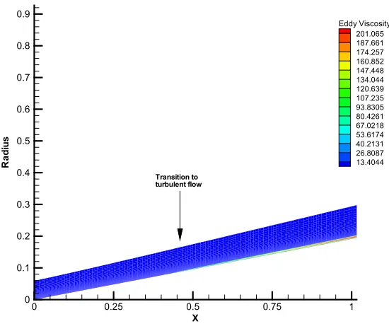
Section 2. Figure 17 confirms this formulation in a body-length cross sectional contour cut of the eddy viscosity. Beyond the distance specified by the transition criteria as the transition onset location, the eddy viscosity grows rapidly close to the surface of the cone as viscous effects start to dominate this region. This growth in eddy viscosity is responsible for the extra fluid heating around the surface in the turbulent flow as described in Section 4.4.

4.6 Comparison of Methods

As is discussed in Section 3.3, three different versions of the time scale characteristic of non-turbulent fluctuations were run for each transitional Reynolds number: 1.98x106/ft, 1.03x106/ft, 7.8x105/ft, and 6.09x105/ft. The first was done using the ISDE method with an average turbulent intensity of 1.5. Secondly, a simulation set was performed using the BLES method developed in this paper with an average turbulent intensity of 1.5. Lastly, the four cases were simulated with the BLES technique and

(36)

revealed in this plot. The difference in the time scale constant c2 in Equation (2.10) when

using a value of Tu=1.5 versus Tu=1.575 is only 0.012. Yet, even with such a small difference in the constant, an obvious difference appears in the time scale plot.

Figures 19, 20, 21, and 22 present heat flux distributions for Re/L=1.98x106/ft using the three different versions of the time scale. Figures 23, 24, and 25 are similar plots for a Reynolds number of 1.03x106/ft. Figures 26, 27, and 28 are associated with Re/L=7.8x105/ft and Figures 29, 30 and 31 are with Re/L=6.09x105/ft.

Considering the lowest point on the heat flux curves as the point of transition onset, the onset position in Figure 19 for the 45o curve lags and 88o curve leads the experimental transition location. Nothing can be inferred about the 0o curve because the experimental data points are too few to capture the transition process, which occurs very close to the nose of the cone. The extent and magnitude of the transition region along the 45o curve matches well with the experimental data. The peak heat flux at the 88o curve is noticeably higher than in the experimental data but nothing can be inferred about the extent of the transitional region at this location since the transitional region extends past the end of the cone. In Figure 20, the transition onset location for the 45o_{station closely}

matches the experimental transition onset location, magnitude and extent while the 88o curve resembles the same curve in Figure 19, but with an even larger peak value. Oscillations in this curve are associated with pressure oscillations emanating from the conical shock. Figure 21 is similar to the curves found in Figure 20 with the exception that the 88o_{and 45}o_{curves have moved forward slightly. The 45}o_{curve is still a good}

approximation of the experimental transition curve.

(37)

To check the validity of the model in the laminar, transitional, and turbulent regions of the flow, the 45o curve from the last method at Re/L=1.98x106/ft is compared against fully laminar and turbulent curves at the same location along the cone in Figure 22. The model performs well at predicting the heat flux in the laminar and turbulent regions of the flow. The transitional region successfully raises the laminar heat flux up to the turbulent values after peaking around the center of the transitional zone.

In Figure 23, corresponding to Re/L=1.03x106/ft, the 0o curve transitions reasonably close to the experimental data, although the fully turbulent level of the heat flux is lower than the experimental value. The 45o curve lags well behind the experimental data, so much so that the extent and magnitude of transition cannot be compared with experimental data. In accord with experimental data, heat flux predictions at 88o indicate fully laminar flow for this Reynolds number and for lower values. The curves in Figure 24 better follow the experimental data, with the 0o curve matching the experimental transition onset location, but the 45o curve still lags the experimental onset position. Like the ISDE method at 0o, the BLES technique does not produce a high enough heat flux in the transitional region. Increasing Tu to a value of 1.575 in Figure 25 moves the transition onset position at 45o further forward, bringing the prediction in closer agreement with the experimental data. The onset position at 0o is undisturbed, and laminar flow is still indicated at θ =88o. Only the 45o curve transition region magnitude is similar to the data. As with the previous calculations, the magnitude of the heat flux is under-predicted in the transitional region.

Similar trends hold for Re/L=7.8x105_{/ft as seen in Figures 26, 27 and 28. The}

(38)

calculation predicts that the 45o curve becomes fully laminar while the experimental data would suggest otherwise. The 0o curve again under-predicts the magnitude of the heat flux in the transitional region. Figure 27 shows that the use of the BLES method shifts the transition onset locations in Figure 26 forward, but not to the levels indicated in the experimental data. Increasing the average turbulent intensity in Figure 28 brings the onset positions within range of the experimental data, but the calculations still under-predict the heat flux values in the transitional regime.

In Figures 29, 30 and 31, corresponding to a Reynolds number of 6.09x105/ft it is clear that none of the variants of the model adequately predict transition onset, placing the onset position further downstream then indicated in the experimental data. The trends evident earlier continue to hold with the ISDE technique predicting transition onset further downstream than the other models.

5 CONCLUSIONS 5.1 Conclusions

The findings of the last section are summarized in Table 2 with respect to each of the time scale calculation methods. The model performs reasonably well for higher Reynolds numbers, but its accuracy starts to deteriorate around the lower end of the spectrum of Reynolds numbers evaluated. Transition onset location was accurately simulated using the third version of the time scale, but the magnitude of the heat flux curves in the transition region of the flowfield is not as accurate.

For all transitional runs performed, the 0o heat fluxcurve is under-predicted in the transitional region of the code when compared with experimental data, and with respect

(39)

to the Re/L=1.98x106/ft case, the calculated 88o heat flux curve is too high. There are two possibilities for the source of the discrepancy. The first is based on the fact, as was determined in Reference [6], that the non-turbulent section of the model is independent of the turbulent model, but the opposite is not true. If the non-turbulent and transitional sections of the code do not produce the correct environment for the turbulence model to function correctly, then a low eddy viscosity output will result. This in turn would not produce the flow properties common to turbulent flow and could ultimately prevent the heat flux from reaching the maximum it should. Since the 88o heat flux curve tended to rise well above experimental values for the Re/L=1.98x106/ft case, it is possible that the opposite can also be true. The non-turbulent/transitional portion of the model could result in too much eddy viscosity growth in this region of the flow, leading to the observed over-prediction of the heat flux and the forward shift of the onset location. The second possibility is that the performance of the model in the transitional region (0<Γ<1)

is inadequate. In past work [6], it was shown that C_t in the C_t

(

1−Γ

)

v~Ω term in

Equation (2.20) is likely a flow-dependent quantity in that it needs to be adjusted for higher-sped flows to ensure best agreement with experimental data. It is possible that a better modeling of this term is necessary.

(40)

small change in this value drastically changes the results of the model. Therefore, such assumptions as were made in Reference [4] about c2 in Equation (3.3) are not valid with

this one-equation transition/turbulence model due to its high sensitivity to Tu.

Overall, the one-equation transition/turbulence developed in this paper using a boundary layer edge search to locate boundary layer edge values and a value of 1.575 for the average turbulent intensity produced the best results at simulating transitional flows over the elliptic cone. The resulting three-dimensional, high turbulent intensity model is considered reasonably accurate for Reynolds numbers between 1.98x106/ft and 7.8x105/ft in locating transition onset location and extent, but it performs poorly at predicting fluid flow properties within the transitional region.

(41)

LIST OF REFERENCES

[1] Warren, E.S., and Hassan, H.A., “An Alternative to the en Method for Determining Onset of Transition,” AIAA Paper 97-0825, January, 1995.

[2] Dhawan, S. and Narasimha, R., Some Properties of Boundary Layer Flow During Transition from Laminar to Turbulent Motion,” Journal of Fluid Dynamics, Vol. 3, No. 4, 1958, pp. 418-436.

[3] McDaniel, R.D., Nance, R.P., Hassan, H.A., “Transition Onset Prediction for High Speed Flow,” AIAA Paper 99-3792, June, 1999.

[4] Xiao, X., Edwards, J.R., and Hassan, H.A., “Transitional Flow over an Elliptic Cone at Mach 8,” Journal of Spacecraft and Rockets, Vol. 38, No. 6, 2000, pp. 941-945. [5] Kimmel, R.L., Poggie, J., and Schwoerke, S.N. “Laminar-Turbulent Transition in a

Mach 8 Elliptic Cone Flow,” AIAA Journal, Vol. 37, No. 9, pp. 1080-1087.

[6] Edwards, J.R., Roy, C.J., Blottner, F.G., and Hassan, H.A. “Development of a One-Equation Transition / Turbulence Model,” AIAA Paper 2000-0133, January, 2000. [7] Spalart, P.R. and Allmaras, S.R., “A One-Equation Turbulence Model for

Aerodynamic Flows,” La Recherche Aerospatiale, Vol. 1, 1994, pp. 5-21. [8] Edwards, J.R., “Advanced Implicit Methods for Finite-Rate Hydrogen-Air

(42)

APPENDIX

Appendix 1: Spalart-Allmaras Turbulence Model

The equation is written in terms of eddy viscosity with eight closure coefficients and three closure functions.

(

)

(

)

(

)

        ∂ ∂ − ∂ ∂ = = Ω + Ω = Ω Ω = − + = =       + + = + − = + = = = = + + = = = = =         ∂ ∂ +         ∂ ∂ + ∂ ∂ +       − Ω = i j j i ij ij ij v w w w w v v v v w w b b w v b b j b j j w w b x U x U S S S f d v d v r r r C r g v v C g C g f f f C f C C C C C C C C x v C x v v v x d v f C v C Dt v D 2 1 2 , ~ ~ ~ ~ , , ~ 1 , 1 1 , 41 . 0 , 2 , 3 . 0 , 1 3 / 2 , 1 . 7 , 622 . 0 , 1355 . 0 ~ ~ ~ 1 ~ ~ ~ ~ 2 2 2 2 2 6 2 6 / 1 6 3 6 6 3 1 2 3 1 3 3 1 3 2 2 2 1 1 1 2 1 2 2 2 1 1 κ κ χ χ χ χ χ κ σ κ σ σ σ where

d: distance to nearest wall

ft2: turbulence function fv1: wall damping function fw: wall blockage function

Sij: rotation tensor t: time

U: velocity

κ: von Karman constant (0.41) ν : non-turbulent viscosity

ν~: turbulent viscosity (working varilable) Ω: rotation tensor magnitude

χ: ratio of turbulent and laminar viscosities

(43)

TABLES

Table 1: Freestream properties for simulations

Pressure (Pa) Density(kg/m^3) Viscosity Velocity (m/s) Tinf(K) Tw/Tinf Mach Number Re/m Re/ft Gamma

300.68 0.0194 3.49E-06 1168 53.62 5.7 7.93 6496290.96 1980576.51 1.4

156.37 0.0101 3.49E-06 1168 53.62 5.7 7.93 3378400.00 1030000.00 1.4

118.30 0.0076 3.49E-06 1168 53.62 5.7 7.93 2555910.67 779241.06 1.4

92.45 0.0060 3.49E-06 1168 53.62 5.7 7.93 1997520.00 609000.00 1.4

Table 2: Transition location and magnitude with respect to experimental data

Re/ft t-location t-magnitude t-location t-magnitude t-location t-magnitude

1.98E+06 Behind Good In Front High

1.03E+06 Good Low Behind Good Good

7.80E+05 Behind Low Behind Good Good

6.09E+05 Behind Behind Good Good

1.98E+06 Good Good In Front High

1.03E+06 Good Low Behind Good Good Good

7.80E+05 Behind Low Behind Good Good Good

1.98E+06 Good Good In Front High

1.03E+06 Good Low Good Good Good Good

7.80E+05 Good Low Good Good Good Good

0o 45o 88o

0o ₄₅o ₈₈o

ISDE, Tu=1.5

BLES, Tu=1.5

BLES, Tu=1.575

(44)

FIGURES

0 0.1 0.2

0 0.1 0.2 0.3 0.4 0.5 0.6 0.7 0.8 0.9 1 0

0.1 0.2

0.3

Z

Y

X

θ = 0ο

θ = 90ο k

j i

Figure 1: Elliptic cone grid orientation

u (m/s)

d

ist

a

n

ce

fr

o

m

sur

fa

ce

(m

)

0 500 1000

0 0.01 0.02 0.03 0.04 0.05 0.06 0.07 0.08

conical shock

Figure 2: Velocity distribution, X=0.04m, θ =61.7o (Re/L=1.98x106/ft, transitional)

(45)

pressure (N/m2₎

d

ist

a

n

ce

fr

o

m

sur

fa

ce

(m

)

200 300 400 500

0 0.01 0.02 0.03 0.04 0.05 0.06 0.07 0.08

conical shock

Figure 3: Pressure distribution, X=0.04m, θ =61.7o (Re/L=1.98x106/ft, transitional)

ρ

d

ist

a

n

ce

fr

o

m

sur

fa

ce

(m

)

0 10 20

0 0.01 0.02 0.03 0.04 0.05 0.06 0.07 0.08

u (kg/(m2_s)) BL edge

conical shock

(46)

Iteration

R

e

si

dua

l

1000 2000 3000 4000

10-11

10-9

10-7

10-5

10-3

Fully Laminar Fully Turbulent

Figure 5: Convergence history

(Re/L=1.98x106/ft, fully laminar and turbulent)

Iteration

Re

si

d

u

a

l

1000 2000 3000 4000

10-9

10-8

10-7

10-6

10-5

10-4

10-3

10-2

10-1

100

ISDE, Tu=1.5 BLES, Tu=1.5 BLES, Tu=1.575

Figure 6: Turbulent residual norm history (Re/L=1.98x106/ft, transitional)

(47)

Iteration

Re

si

d

u

a

l

1000 2000 3000 4000

10-9

10-7

10-5

10-3

10-1 ISDE, Tu=1.5

BLES, Tu=1.5 BLES, Tu=1.575

Iteration

Re

si

d

u

a

l

1000 2000 3000 4000

10-9

10-7

10-5

10-3

10-1 ISDE, Tu=1.5

BLES, Tu=1.5 BLES, Tu=1.575

(48)

Iteration

Re

si

d

u

a

l

1000 2000 3000 4000

10-9

10-7

10-5

10-3

10-1 ISDE, Tu=1.5

BLES, Tu=1.5 BLES, Tu=1.575

Y

Z

0 0.1 0.2 0.3

0 0.05 0.1 0.15 0.2

0.25 1700.62

1607.29 1513.96 1420.63 1327.3 1233.97 1140.64 1047.31 953.982 860.652 767.322 673.992 580.662 487.332 394.002 Pressure (Pa)

Figure 10: Pressure distribution X=0.933m (Re/L=1.98x106/ft, fully laminar)

(49)

Y

Z

0 0.1 0.2 0.3

0 0.05 0.1 0.15 0.2

0.25 334.399

315.68 296.961 278.243 259.524 240.806 222.087 203.368 184.65 165.931 147.212 128.494 109.775 91.0565 72.3379 Temperature (K)

Figure 11: Temperature distribution X=0.933m (Re/L=1.98x106/ft, fully laminar)

Y

Z

0 0.1 0.2 0.3

0 0.05 0.1 0.15 0.2

0.25 336.105

317.273 298.44 279.608 260.775 241.943 223.111 204.278 185.446 166.614 147.781 128.949 110.117 91.2843 72.4519 Temperture (K)

(50)

Re_x

qw

(B

T

U

/f

t

2/s

)

2E+06 4E+06 6E+06

0 0.5 1 1.5 2 2.5 3 3.5

Comp Comp Comp

θ=88ο

θ=00

θ=45ο

Figure 13: Heat flux distribution along rays of cone (Re/L=1.98x106/ft, fully laminar)

Re_x

qw

(B

T

U

/f

t

2/s

)

2E+06 4E+06 6E+06

0 0.5 1 1.5 2 2.5 3 3.5

Comp Comp Comp

θ=88ο

θ=00

θ=45ο

Figure 14: Heat flux distribution along rays of cone (Re/L=1.98x106/ft, fully turbulent)

(51)

i

j

50 100

10 20 30 40 50 60 70 80 90 100 110

1581.96 1468.97 1355.97 1242.97 1129.97 1016.98 903.98 790.982 677.985 564.987 451.99 338.992 225.995 112.997 0

ν/(νntxCµ)

Figure 15: Transition criteria over elliptic cone (Re/L=1.98x106/ft, Tu=1.575)

i

j

50 100

10 20 30 40 50 60 70 80 90 100 110

1 0.928571 0.857143 0.785714 0.714286 0.642857 0.571429 0.5 0.428571 0.357143 0.285714 0.214286 0.142857 0.0714286 0

Γ

(52)

X

R

a

di

us

0 0.25 0.5 0.75 1

0 0.1 0.2 0.3 0.4 0.5 0.6 0.7 0.8 0.9

201.065 187.661 174.257 160.852 147.448 134.044 120.639 107.235 93.8305 80.4261 67.0218 53.6174 40.2131 26.8087 13.4044 Eddy Viscosity

Transition to turbulent flow

Figure 17: Viscosity distribution θ=63o (Re/L=1.98x106/ft, transitional, Tu=1.575)

Degrees

τ

20 40 60 80

1E-07 2E-07 3E-07 4E-07 5E-07 6E-07 7E-07 8E-07 9E-07 1E-06 1.1E-06

ISDE, TU=1.5 BLES, Tu=1.5 BLES, Tu=1.575

nt

Figure 18: Non-turbulent time scale X=0.060m (Re/L=1.98x106/ft, transitional)

(53)

Re_x

qw

(B

T

U

/f

t

2/s

)

2E+06 4E+06 6E+06

0 0.5 1 1.5 2 2.5 3 3.5

Exp Comp Exp Comp Exp Comp

θ=88ο

θ=00

θ=45ο

Figure 19: Heat flux distribution along rays of cone (Re/L=1.98x106/ft, ISDE, Tu=1.5)

Re_x

qw

(B

T

U

/f

t

2/s

)

2E+06 4E+06 6E+06

0 0.5 1 1.5 2 2.5 3 3.5

θ=88ο

θ=00

θ=45ο

(54)

Re_x

qw

(B

T

U

/f

t

2/s

)

2E+06 4E+06 6E+06

0 0.5 1 1.5 2 2.5 3 3.5

θ=88ο

θ=00

θ=45ο

Figure 21: Heat flux distribution along rays of cone (Re/L=1.98x106/ft, BLES, Tu=1.575)

Re_x

qw

(B

T

U

/f

t

2/s

)

2E+06 4E+06 6E+06

0 0.5 1 1.5 2 2.5 3 3.5

Laminar Turbulent Transition

Figure 22: Heat flux distribution along ray of cone (Re/L=1.98x106/ft, θ=450, Tu=1.575)

(55)

Re_x

qw

(B

TU

/f

t

2/s

)

1E+06 2E+06 3E+06

0 0.2 0.4 0.6 0.8 1 1.2 1.4 1.6 1.8 2 2.2

2.4 Exp

Comp Exp Comp Exp Comp

θ=00

θ=88ο

θ=45ο

Figure 23: Heat flux distribution along rays of cone (Re/L=1.03x106, ISDE, Tu=1.5)

Rex qw

(B

TU

/f

t

2/s

)

1E+06 2E+06 3E+06

0 0.2 0.4 0.6 0.8 1 1.2 1.4 1.6 1.8 2 2.2

2.4 Exp

θ=00

θ=88ο

θ=45ο

(56)

Re_x

qw

(B

TU

/f

t

2/s

)

1E+06 2E+06 3E+06

0 0.2 0.4 0.6 0.8 1 1.2 1.4 1.6 1.8 2 2.2

2.4 Exp

θ=00

θ=88ο

θ=45ο

Figure 25: Heat flux distribution along rays of cone (Re/L=1.03x106/ft, BLES, Tu=1.575)

Re_x

qw

(B

T

U

/f

t

2/s

)

500000 1E+06 1.5E+06 2E+06 2.5E+06

0 0.5 1 1.5 2

θ=88ο

θ=45ο

θ=00

Figure 26: Heat flux distribution along rays of cone (Re/L=7.8x105/ft, ISDE, Tu=1.5)