Solving Complex Modeling of System-on-a-Chip (SOC) Test Automation and Optimal Resource Allocation by Neural Networks

(1)

ABSTRACT

KLOYPAYAN, JIRAWAN. Solving Complex Modeling of System-on-a-Chip (SOC) Test Automation and Optimal Resource Allocation by Neural Networks. (Under the direction of Professor Yuan-Shin Lee.)

The objective of this research is to optimize the testing time and test resource allocation for System-on-a-Chip (SOC). The mathematical formulation and the neural networks with different techniques are proposed to solve these SOC test problems. First, a

(2)

(3)

Solving Complex Modeling of System-on-a-Chip (SOC) Test

Automation and Optimal Resource Allocation by Neural

Networks

By

Jirawan Kloypayan

A dissertation submitted to the Graduate Faculty of

North Carolina State University

in partial fulfillment of the requirements for the Degree of

Doctor of Philosophy

INDUSTRIAL ENGINEERING

Raleigh 2002

APPROVED BY

__________________ Dr. Yuan-Shin Lee Chair of Advisory Committee

__________________ __________________

Dr. Ezat T. Sanii Dr. Robert E. Young

Advisory Committee Advisory Committee

__________________ __________________

(4)

BIOGRAPHY

(5)

ACKNOWLEDGMENTS

I would like to express my sincere appreciation and gratitude to my advisor, Dr. Yuan-Shin Lee, for his valuable guidance and assistance throughout this research. I would like to extend my appreciation to Dr. Krisnendu Chakrabarty for his time, helpful encouragement and advice. I appreciate the constructive suggestions and comments from my graduate committee: Dr. R. Young, Dr. E. T. Sanii and Dr. Elmor Peterson.

I would also like to express my thanks to my research groupmates: John, Bahattin, Susana, Yongfu, Abhinand, Weighang and Ron, for their valuable suggestions during group meetings and personal discussions. I would like to extend my gratitude to Dr. Jun, Dr. Yau and Dr. Ju for instructive discussions during their visit. I would also like to specially thank Saowanee, Phoemphun, and Teerada for their friendship in going through this phase of time with me.

I would also like to express my gratitude to the Royal Thai Government. Without the support from Royal Thai Government, it would not be able for me to do this research for Ph.D. degree in the U.S.

(6)

LIST OF TABLES

Page

Table 2.1 Test data of the cores for the SOC system S1. . . 28

Table 2.2 Test data of the cores for the SOC system S2 and S3. . . 31

Table 2.3 The SOC test scheduling solutions from the proposed NN after 20 runs. . 35

Table 3.1 Test data of the core for the SOC system S4. . . 50

Table 3.2 The results from using the proposed maximum neural network applied to the example SOC system S4 with three TAMs. . . 51

Table 4.1 Test data for each core in SOC chip d695. . . 69

Table 4.2 The best solution of SOC testing time, width allocation and core assignment for the SOC system d695 with three TAMs. . . 70

Table 5.1 The results from using the proposed maximum neural network applied to the example SOC system S4 with two TAMs . . . 74

Table 5.2 Comparison of the SOC testing time for different methods. . . 76

Table 5.3 The results from using the proposed maximum neural network applied to the example SOC system S4 with four TAMs. . . 77

Table 5.4 The best solutions of testing time for the system S4 when the number of TAM lines are varying. . . . . . . . 77

Table 5.5 The testing time for the system S2 with the power constraint when the total TAM widths are varying (the maximum power is 100 mW). . . . 79

Table 5.6 The testing time for the system S2 with the power constraint when the maximum power dissipation is varying (the total TAM width = 28). . . 79

Table 5.7 Test data for each core in SOC chip g1023. . . 83

Table 5.8 Test data for each core in SOC chip p34392. . . 83

(10)

without power constraint for the example system d695 with two TAMs. . . 90 Table 5.13 The comparison of SOC testing time and computation time with and

(11)

LIST OF FIGURES

Page

Figure 1.1 An example of System-on-a-Chip (SOC). . . 4

Figure 2.1 Picture of an example System-on-a-Chip (SOC) design and testing. . . 23

Figure 2.2 An example of a generic core-based system with one external test bus, and shared and dedicated BIST logic for the cores. . . . . . . 23

Figure 2.3 A single-layer neural network. . . 24

Figure 2.4 A neural unit in the neural network. . . 24

Figure 2.5 The proposed Neural Network. . . 25

Figure 2.6 The proposed structure of a general constraint (PC, RC, CC) unit. . . . 26

Figure 2.7 The proposed structure of a power constraint (PoC) unit. . . 26

Figure 2.8 The proposed searching and optimizing algorithm for SOC test scheduling. . . 27

Figure 2.9 The SOC System S1 with 8 cores. . . 28

Figure 2.10 The best result test schedule for the system S1, with only RC and CC constraints. . . 29

Figure 2.11 The best result test schedule for the system S1, with RC, CC and PC constraints. . . 29

Figure 2.12 A feasible test schedule for the system S1, with all the constraints RC, CC, PC, and PoC. . . 30

Figure 2.13 The best result test schedule for the system S1, with all the constraints RC, CC, PC, and PoC after eliminating the idle time by the proposed method. . . . . . . . 30

Figure 2.14 The second example of the SOC system S2 with 13 cores. . . 31

Figure 2.15 The best result test schedule for the system S2 with all the constraints RC, CC, PC, PoC. . . 32

Figure 2.16 The third example of the SOC system S3 with 20 cores. . . 33

(12)

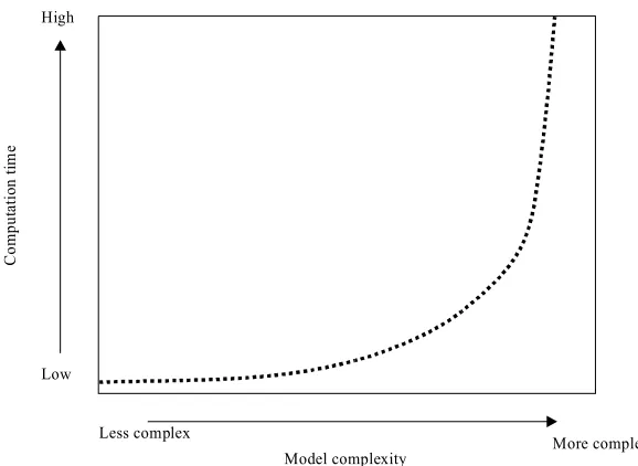
CC, PC, and PoC. . . 34 Figure 3.1 An example of core-based SOC system with two TAM lines. . . 47 Figure 3.2 An example of general maximum neural network. . . 48 Figure 3.3 The relation of the computation time and the SOC model complexity

(Using the traditional method to solve NP-complete problems). . . 48 Figure 3.4 The proposed neural network architecture. . . 49 Figure 3.5 The proposed searching and optimizing algorithm for SOC test design. . 49 Figure 3.6 TAM design and test scheduling for the system S4 with three TAMs

and the total TAM width of 44. . . 52 Figure 4.1 Embedded core test infrastructure for SOC testing. . . 65 Figure 4.2 An example of a core with wrapper. . . 65 Figure 4.3 An example of wrapper scan chain design by the PTI and LPT algorithm. . 66 Figure 4.4 The proposed maximum neural network (MNN) architecture. . . 67 Figure 4.5 The proposed MNN searching and optimizing algorithm for

SOC test design. . . 68 Figure 4.6 Test Access Mechanism (TAM) design for the SOC system d695

with three TAMs and total TAM width W is equal to 28 bits. . . 70 Figure 5.1 TAM design and test scheduling for the system S4 with two TAMs

and the total TAM width of 20. . . . . . 75 Figure 5.2 The comparison of SOC testing time for SOC system S4 with two TAMs

using different methods . . . 76 Figure 5.3 The relationship of the total SOC testing time and the number of

TAM lines and the total TAM width. . . 78 Figure 5.4 The comparison of SOC testing time for SOC d695 with two TAMs using

Integer Linear Programming (ILP), PPAW-enumerate, and the proposed MNN. . 86

Figure 5.5 The comparison of the computation time of different methods when the

number of SOC cores is increased. . . . 87 Figure 5.6 The comparison of the computation time of different methods when

(13)

Figure 5.7 The SOC testing time (objective) and the computation time of

the proposed MNN when the number of iterations varies. . . 88 Figure 5.8 The comparison of SOC testing time for the example system d695

with three TAMs using Integer Linear Programming (ILP), PPAW-enumerate,

ECTSPSol, and the proposed MNN. . . 89 Figure 5.9 The comparison of SOC testing time for the example system p93791

with three TAMs using PPAW-enumerate, ECTSPSol, and the proposed MNN. 89

Figure 5.10 The comparison of SOC testing time and computation time for

(14)

CHAPTER 1 INTRODUCTION

Currently, the advances in semiconductor technology have led to more complex

System-on-a-Chip (SOC) designs. The SOC sizes range from 20-50 million transistors, with integrated logic, dynamic random access memory (DRAM), and analog [Shaikh 00]. Because of the high complexity and high density of the SOC system, testing SOC problems becomes crucial. In this research, we investigate new soft computing tools to solve the complex SOC test automation problems. In the following sections, System-on-a-Chip design and testing are introduced.

1.1 System-on-a-Chip (SOC) Testing

In the semiconductor industry, a new system design, called System-on-a-Chip (SOC) design, is currently being introduced to use multiple embedded modules built on a single chip. With today’s technology, a single chip can consist of millions of transistors or components [Chauhan 00, Aikyo 00]. Figure 1.1 shows an example of SOC. To design a SOC system on a single chip, a designer often uses pre-designed, reusable mega cells known as cores in the SOC design [Chandramouli 96]. Embedding the cores onto SOC increases the width of the system bus and thus increases overall system performance, i.e., it can offer higher speed and lower power consumption [Daeje 98, Shubat 01]. A core can be defined as a complex piece of reusable module design such as microprocessors, bus interface, and memories [Crouch 99]. Cores are usually provided by the core providers and are treated as

(15)

designed, manufactured, and tested by a component provider before sending it to a system integrator. Unlike system-on-board, a core is only a description of a module and is not yet manufactured when it is sent to a system integrator. A core integrator receives cores from each core provider and integrates cores at the chip-level and tests them using SOC testing mechanisms [Rajsuman 00]. Because of the design complexity and the huge number of components in the System-on-a-Chip design, testing of the SOC design becomes critical for the semiconductor industry.

Zorian et al. introduced generic conceptual test access architecture for embedded core [Zorian 99]. There are three elements in the embedded core test infrastructure; (i) test pattern source and sink, (ii) test access mechanism (TAM), and (iii) core test wrapper. A test pattern source generates test stimuli for an embedded core. A test pattern sink compares the responses from an embedded core to the expected responses. A test pattern source and sink can be designed either off-chip, using external automatic test equipment (ATE), or on-chip, using built-in-self test (BIST), or a combination of both [Zorian 99]. A BIST provides better accuracy and performance-related defect coverage, but it also increases the silicon area. The test patterns generated from a test pattern source are transported by test access mechanism (TAM) to a core under test. A TAM also transports the test stimuli from a core under test to a test pattern sink. A core test wrapper is an interface between a core and the system in which the core is embedded. The wrapper provides the switching between normal functional access and test access via the TAM [Marinissen 00].

(16)

1.2 Problems Description

In this dissertation, three major research issues of the SOC test automation are investigated. First, by considering a SOC system consisting of main test resources such as external test and built-in-self-test (BIST), the SOC test scheduling is studied to minimize the SOC testing time subject to different constraints: (i) precedence constraint, (ii) resource constraint, (iii) core constraint, and (iv) power constraint. Second, a maximum neural network (MNN) is proposed to solve the test resource allocation problems for SOC. Third, after core wrapper design, the SOC test automation problems with resource allocation are studied to minimize the total SOC testing time. In this research, developing soft computing techniques of an unsupervised maximum neural network (MNN) are proposed to optimize the overall SOC testing time with core wrapper design and optimal resource allocation.

1.3 Outline of Dissertation

(17)

(18)

CHAPTER 2 USING NEURAL NETWORK WITH FIXED-WEIGHT NET IN

MODELING AND SOLVING THE SYSTEM-ON-A-CHIP (SOC) TEST

SCHEDULING

This chapter presents the modeling and the proposed solution approach for solving the new System-on-a-Chip (SOC) design test scheduling problems. To solve the SOC test design problems, a neural network (NN) combined with heuristic algorithm has been developed. The SOC design test scheduling and optimization are subject to four different constraints: (i) precedence constraint, (ii) resource constraint, (iii) core constraint, and (iv) power constraint. The results demonstrate that the developed model with the soft computing techniques can successfully solve a large size SOC test scheduling problem within a reasonable time. The techniques presented in this chapter can be used for the optimization of the SOC design testing that is important for current development in the semiconductor and electronics industry.

2.1 Introduction

(19)

once as part of the overall system-chip design, which is quite different from a conventional system-on-board (SOB) test that traditionally takes multiple tests [Zorian 98]. In Figure 2.2, cores 1, 2, 3 and 4 are tested using either external-test or BIST logic. Core 5 is tested using only BIST, and core 6 is tested using only external-test. In Figure 2.2, cores 1, 2 and 5 have their own dedicated BIST logics. On the other hand, cores 3 and 4 share a BIST logic.

When a SOC system designer/integrator gets cores from a core provider, he/she encounters two major tasks in solving the SOC test problems. The first task is how to design a test access mechanism (TAMs), and the second task is how to find the test scheduling for an SOC system to minimize the time-to-market. TAMs must be designed to transport the pre-computed tests from system I/Os to core I/Os [Iyengar 01b]. Test scheduling determines the order in which the various cores are tested and what testing resources are used for SOC testing subject to a variety of hardware, capacity and sequence constraints. There are some researchers studying the first issue of the TAM design, but very few are studying the SOC test scheduling problems [Chakrabarty 00c].

In this chapter, we focus on the research of finding the optimal solution for solving the SOC test scheduling problems. The objective of the SOC cores test scheduling is to minimize the total SOC testing time subject to the following constraints:

(i) Resource conflicts between cores that share the same test component (i.e., TAMs or BIST logics),

(ii) Core conflicts between test components that are used to test that core, (iii) Precedence constraints among different tests, and

(iv) Power consumption constraints of the test system.

(20)

for minimizing core-based system LSI testing time based on a combination of both external-test and BIST for each core [Sugihara 98]. In the earlier work, Chakrabarty (2000) proposed a method using integer linear programming (ILP) to minimize the SOC testing time with various constraints without any redesign of the embedded cores [Chakrabarty 00a, Chakrabarty 00b, Chakrabarty 00c]. In Chakrabarty’s (2000) work presented in [Chakrabarty 00a], a method of TESTRAIL was proposed as a test access mechanism (TAM), which can provide access to one or more cores. The results showed that these SOC test problems are NP-hard problems [Chakrabarty 00a, Chakrabarty 00c, Iyengar 01b].

When solving the SOC testing problems by using linear programming, as the size of problem increases, there is a polynomial growth in the number of constraints and variables [Flores 99]. Using heuristic methods does not guarantee the optimal solution when the size of problems increases [Dagli 94]. Since the search of the entire space is often intractable due to the number of possible solutions, finding the optimal solution becomes difficult to achieve.

In this chapter, we investigate the modeling and the soft computing techniques to solve the SOC test scheduling problems. After the formulation of the SOC design testing problems, a neural network (NN) combined with heuristic random search method (tabu search) is proposed to minimize the testing cost that occurred during SOC testing.

2.2 Neural Network (NN) for Adaptive Learning and Optimization

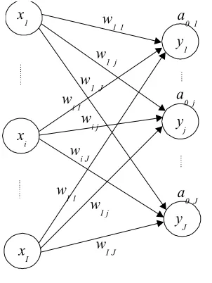
Recently, neural networks (NNs) have been used in solving scheduling problems. A neural network is a system constructed to mimic the functions of a brain. A neural network consists of a system of individual neural units with weighted interconnections, as shown in Figure 2.3. Each neural unit consists of nodes linked together with the associated weights between each node. There are several types of neural networks [Dagli 94]. Figure 2.3 shows one type of neural networks called single-layer neural network, which consists of only input units and output units. In Figure 2.3, an associated weight wij connects an input unit xi with

an output unit yj. Each output unit yj has a bias term a0j. Figure 2.4 shows a neural unit in a

(21)

added and then passed through an activation function [Dagli 94, Lee 00]. In general, each neural unit consists of two parts: a linear summation Sj and a nonlinear activation function

f(Sj), and they can be formulated as follows (also shown in Figure 2.4) [Kartalopoulos 96]:

(

)

j

I

i

i ij

j w x a

S ₀

1

+ × =

=

(2.1)

) ( _j j f S

y = (2.2)

where xi is the input i to a neural unit, i= 1, …, I;

yj is the output j from the neuron unit, j = 1,…,J;

wij is the weight associated with each input unit i and output unit j; and

a0j is the bias value for an output j.

A neural network can be classified into three categories by different training types: supervised training, unsupervised training and fixed-weight nets [Fausett 94]. In a supervised training NN, the training is done by adjusting the weights according to a learning algorithm. The weights are adjusted until the difference of the actual outputs and the target outputs is less than or equal to the desired error. In an unsupervised training NN, the weights are adjusted without the use of target outputs. The outputs from an unsupervised NN are classified into sets without being compared to a desired output. In a fixed-weight NN, the weights are fixed and set to represent the constraints and the quantity to be maximized or minimized. Neural networks have been used in solving the job shop scheduling problems [Flores 99, Foo 88, Yu 97, Jain 98, Lee 00, Yang 00]. For example, Yang, et al. (2000) proposed a NN in solving job-shop scheduling problems that satisfy three constraints: a job constraint, a machine constraint and a precedence constraint [Yang 00]. In his paper, the precedence constraint is among the operations of the same job and a starting time unit considers release time and due date of each job.

(22)

[Flores 99]. However, using the neural network approach alone may not get the optimal solution [Jain 98]. This is due to its lack of generic pattern between inputs and outputs in solving the optimization problems. When solving larger size optimization problems, using only neural networks has been identified to be insufficient [Jain 98, Lee 00]. Hybrid technologies that combine the neural network with other strategies such as tabu search or simulated annealing may lead to better solutions with a more reasonable computational time. Although neural networks may not be as effective as the conventional optimization methods, they offer advantages in dealing with large scales optimization problems [Lee 00, Sabuncuoglu 96]. They can quickly find near optimal solutions when solving large size optimization problems [Fausett 94, Lee 00].

In this chapter, a neural network combined with heuristic random search is proposed to solve the SOC core test scheduling problems. Details of how to model the SOC test scheduling problems by using the neural network approach are presented in the following sections.

2.3 Formulation of the SOC Core Test Scheduling Problems

In this chapter, we consider the problems in which the SOC core-based systems are tested by using either external-testing, BIST or combination of both test resources, as shown earlier in Figure 2.2. To achieve the high fault coverage during SOC testing, a combination of BIST and external-testing must be used as much as possible [Iyengar 01b]. To improve the resource efficiency, BIST logic can be either shared by several cores or dedicated for a specific core, as shown in Figure 2.2. The test sets for all the cores, which include both BIST and external core components, are given. The precedence constraints among cores are also known. To demonstrate the formulation, an example test resource consisting of one external test bus and several Built-in-Self-Tests (BISTs) is used for illustration, as shown in Figure 2.2. The SOC test scheduling problems can be formulated as follows:

Let T = {t11, t12,..., tim, ..., tIM} denote the set of start times for the test patterns

(23)

the test resource (for example, either the external-test bus or BIST), m = 1…M. Let L = {l11,

l12, .., lim, ..., lIM} denote the set of corresponding test lengths for the test sets. The objective

is to find the shortest total testing time for the core-based SOC test design.

To find a feasible SOC test, the conflicts of the resource and core constraints need to be solved. Test sets can be conflicting, if: (i) they share an external test bus at the same time, (ii) they are BIST test sets for cores that share the same BIST resource, or (iii) they are the external and BIST components of the same core’s test set. The conflict between cores i and j

tested on the same test resource m will not occur if and only if either (i) tim −tjm −ljm ≥0, or

(ii) tjm −tim −lim ≥0. This means that the testing periods of both cores (i, j) on the same test

resource (m) cannot be overlapped. On the other hand, the conflict between the test resources m and k for the same core i will not occur if and only if the test periods of core i on the different test resources (m, k) are not overlapped, which is either (i) tik−tim −lim ≥0, or

(ii) 0tim−tik −lik ≥ . The resource constraint and the core constraint are disjunctive

constraints (i.e., multiple alternative constraints). The precedence among cores q and i can occur if tqr −tim −lim ≥0, where core i is tested before core q. To satisfy the power capacity

constraint, the summation of all the power dissipation

=

N

n n

p

1

(for cores that have the

overlapped testing time) cannot exceed the maximum power rating (Pmax) of the test system.

When the SOC test problems are solved, these constraints need to be satisfied [Kloypayan 02a, Kloypayan 02b].

The objective of the SOC test design modeling is to minimize the maximum of the test completion time, i.e., the summation of the starting time tim and the total processing time

lim, subject to all the constraints. The modeling of the SOC core testing can be formulated as

(24)

Objective: minimize C = max{ tim + lim} (2.3)

Subject to: tqr – tim – lim≥ 0, (precedence constraint)

tim – tjm – ljm≥ 0, or tjm – tim – lim≥ 0, (resource constraint)

tim – tik– lik≥ 0, or tik – tim – lim≥ 0, (core constraint)

_max

1

)

( p P

w N

n

n ≤

=

, (power constraint)

{

}

{ }

î í

ì + − >

=

otherwise

t l

t if

w n n n n n

0

0 max

min 1

,n=1,...,N ,

tjm, tik, tim≥ 0,

ljm, lik, lim ≥ 0.

where timis the starting time of core i on a test resource m;

limis the processing time of core i on test resource m;

i, q and j represent a core , i = 1…I, q= 1…I, and j = 1…I;

m, k, r represent a test component, m=1,...,M, k=1,...,M and r=1,...,M ;

pn is the power dissipation that core n consumes while being tested, n=1,...,N;

Pmax is the maximum allowed power dissipation of the testing system; and

N is the number of cores that have the overlapped testing time, N≥ 2.

To solve the SOC core test scheduling problems, a neural network combined with a random search is proposed in this chapter. Details of how to construct the proposed NN and examples of solving the SOC test problems are presented in the following sections.

2.4 Constructing the Neural Network for Solving the SOC Testing Problems

(25)

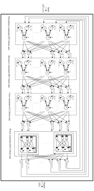
have similar structures, but the fourth unit (PoC unit) has a different structure due to the complex effects of satisfying the power capacity constraint.

As shown in Figure 2.5, the NN receives the inputs of the starting time ST for each core. First, the precedence constraint (PC) units are processed. The PC unit considers the precedence among different cores, which are assumed to be known at the beginning. Then, the starting times of the PC units are adaptively adjusted and sent to the next resource constraint (RC) units, as shown in Figure 2.5. RC units consider that the same test resource cannot test two cores at a time. After the resource constraint is considered, the adjusted starting times from RC units are sent to the core constraint (CC) units, as shown in Figure 2.5. CC units ensure that the same core is not tested on different test resources at a time. After the starting times of all the cores have been adaptively adjusted by the CC units, they are forwarded to the power (PoC) units, as shown in Figure 2.5. Power constraint (PoC) units consider the power consumed by a set of cores having the testing time overlapped, which should not exceed the maximum allowed power rating of the SOC system. The adaptive adjusting procedure repeats until all the constraints have been satisfied, as shown in Figure 2.5. The output of the proposed NN is the set of the scheduled starting times for all the cores. Details of how to construct the constraint units (PC, RC, CC, and PoC units) are discussed in the following two sections.

2.4.1 Constructing the Precedence (PC), Resource (RC) and Core (CC) Constraints

As mentioned earlier in Section 2.2, a neural unit consists of two parts: a linear summation and a nonlinear activation function. In the proposed NN, the linear summation function (S_NN_l) and the nonlinear activator function (NNl) for the constraint units (PC, RC or

CC unit) are defined as follows:

l

l a ex b fy NN

NN w ST u w ST u B

S =( ⋅ ( −1))+( ⋅ ( −1))+ (2.4)

î í ì

< ≥ =

=

0 ,

0 ) (

l l

l

NN NN

l

S if S

f

(26)

) 1 ( )

(u =w ⋅NN +ST u−

ST_ex _c _l _ex (2.6)

) 1 ( )

(u =w ⋅NN +ST u−

ST_fy _d _l _fy (2.7)

where STexis the starting time of cores e on test resource x;

STfy is the starting time of cores f on test resource y;

u is number of iterations, u = 1, 2, …U;

wa, wb, wc, and wd are the weights associated with each node; and

l

NN

B is a bias term.

Figure 2.6 shows a general neural unit of the PC unit, CC unit or RC unit for the proposed neural network. As shown in Figure 2.6, each neural unit takes inputs, which are the starting times )ST_ex(u−1 and ST_fy(u−1) of a pair of the considering testing cores (e, f). As shown in

Equations (2.4)-(2.7), the searching process of this neural unit works as follows. First, the summation function (

l

NN

S ) is calculated by using Equation (2.4) for the summation of the

bias term (B_NN_l) with the multiple terms of starting times, STex(u-1) and STfy(u-1), and their

associated weights wa and wb. Then, the activator function NNl is calculated, as shown in

Figure 2.6. In Equation (2.5), the activator function NNl is set to zero when the constraint

0

≥ l

NN

S is satisfied; otherwise NNl is set to SNN_l.

Equations (2.6) and (2.7) show that, when the given constraint is violated (i.e.,

0

< l

NN

S ), the starting time STex(u-1) of a core e on the test component x is pushed by

(w_c−NN_l) and the starting time STfy(u-1) of a core f on the test component y is pushed by

(w_d −NN_l). Figure 2.6 shows that, when the constraint is violated (i.e., SNN_l <0), the neural

unit sends the adjusted weight wc and wd back to adaptively adjust the starting time STex(u-1)

and STfy(u-1) by using Equations (2.6) and (2.7). If the starting time STfy(u)for core j is less

than 0 (i.e., STfy(u) < 0), the starting time STfy(u) is set to 0. The searching process continues

until all the constraints are satisfied. Figure 2.6 shows that, after satisfying all the constraints, the outputs of the constraint unit are the adaptively adjusted starting times

(27)

In Equations (2.4)-(2.7), all the weights (wa, wb, wc, wd) and the bias term (BNN_l) need

to be determined according to the precedence constraint (PC), the resource constraint (RC) and the core constraint (CC), as defined earlier in Equation (2.3). Based on Equation (2.3), the correspondent weights (wa, wb, wc, wd) and the bias term (BNN_l) for the precedence

constraint (PC) units can be determined as follows:

For PC unit: STex ⇐tqr, STfy⇐tim, and

im NN l

B _l ⇐− ,wa ⇐1,wb⇐−1,wc⇐−1, and wd⇐1. (2.8)

For the resource constraint (RC) units, the correspondent weights (wa, wb, wc, wd) and the

bias term (BNN_l) are determined as follows:

For RC unit: STex ⇐tim, STfy⇐tjm, and

IF (STex≥ STfy)

THEN BNNi ⇐−ljm,wa⇐1,wb⇐−1,wc⇐−1, and wd ⇐1; (2.9)

IF (ST_ex <ST_fy)

THEN BNNi ⇐−lim,wa⇐−1, wb ⇐1, wc ⇐ 1, and wd ⇐−1. (2.10)

For the core constraint (CC) units, the correspondent weights (wa, wb, wc, wd) and the bias

term (BNN_l) can be determined as follows:

For CC unit: STex ⇐tim,STfy⇐tik, and

IF (STex≥ STfy)

THEN BNNi ⇐−lik, wa⇐1, wb⇐−1, wc⇐−1, and wd ⇐ 1; (2.11)

IF (ST_ex <ST_fy)

THEN BNNi ⇐−lim,wa⇐−1, wb ⇐1, wc ⇐ 1, and wd ⇐−1. (2.12)

(28)

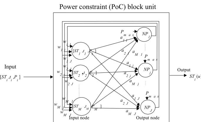
2.4.2 Constructing the Power Constraint (PoC) Unit for the Neural Network

The last constraint for the SOC test model is the power capacity constraint (PoC unit) of the proposed NN. The power constraint (PoC) needs to be considered in the SOC model to limit test concurrency and to ensure that the power rating of the SOC is not exceeded. The concept of the power constraint (PoC) logic is to find groups of cores that have the testing period overlapped. In each group, the summation of the power dissipation of the same group is calculated. If the summation of the power of any group is greater than the maximum power dissipation capacity during testing, the start times of the chosen cores in that group need to be changed to different testing periods. The process continues until every group satisfies the power constraint, i.e., there is no group with the total power dissipation exceeding the maximum power capacity.

Figure 2.7 shows the structure of a power constraint PoC unit in the proposed NN. The number of input nodes is equal to the number of available test resources for a SOC system. As shown in Figure 2.7, the PoC unit takes the input [STi, ti, Pi] of the starting times

STi, the processing times ti, and the power dissipation Pi for a group of the considered testing

cores on different test resources. In Figure 2.7, the number J of the output nodes is set as

[

M

]

M M

M

M _C _C _C

C

J = ₂ + ₃ + ₄ +...+ , where M is the number of the available test resources in the

SOC system. For each PoC unit in the proposed NN, the linear summation function (SP_j)

and the nonlinear activator function (NPj) are defined as follows:

max 1 P P a SP M

i ij i

j = −

= (2.13) )) 1 ( ( max ) ) 1 ( ( min 1

1 − + − −

=

= ST u t ST u

Diff M _i

i i i

M i

j , for ∀aij > 0 (2.14)

î í ì > ≤ = 0 , 0 , 0 j j j j Diff if Diff Diff if

PP (2.15)

î í ì > ≤ = = 0 , 0 , 0 ) ( j j j j j SP if PP SP if SP f

(29)

) 1 ( )

(u =w ⋅NP +ST u−

ST_i _ij _j _i (2.17)

where Pi is the power dissipation of the core tested on test resource i,

i=1,...,M ;

aijis the weights associated with input i and output node j, j = 1,..., J;

Pmax is the maximum power dissipation allowed during testing;

ti is the processing time of core on test resource i;

u is number of iterations, u = 1,…,U;

wij are the weights associated with each node, wij = -1, 0, or 1; and

STiis the starting time of a core on test component i.

After getting the inputs from the groups of cores on different test resources, the summation function SP_j and the nonlinear activator function NPj are calculated by using Equations

(2.13)-(2.17). If the power constraint is violated (i.e., SPj > 0) and the group of inputs is

overlapped (i.e., Diffj >0), the starting times STi of the first core and the last core of the

input cores are adjusted by using Equation (2.17). The weight wij for the first core and the

last core are set to 1 and –1, respectively. On the other hand, all the other weights wij of the

input cores are set to zero, as defined in Equation (2.16). The procedure continues until all the cores satisfy the power capacity constraint in the SOC model, as defined earlier in Equation (2.3).

After all the constraints, i.e., the precedence constraint (PC), the resource constraint (RC), the core constraint (CC) and the power capacity constraint (PoC) have been constructed, they are integrated into the proposed NN for the SOC test system, as shown earlier in Figure 2.5. The complexity of the proposed NN with the different constraints can be found as follows. Assume there are a total of n cores and each core has at most 2 different test resources (i.e., external-test and BIST). The precedence constraint (PC) ensures the cores to be first tested on BIST before using external-test. In Equation (2.3), there are n

(30)

there are only one external-test and one BIST. There are a total of 2*C2n sequence constraint

inequalities, which require 2n(n-1) RC neural units. For the core constraint (CC) neural unit, there are n sequence constraint inequalities, which require n CC units. The total number of interconnections in the proposed neural network is found to be 2n2. The connection complexity of the proposed neural network without power constraint is found to be O(n2). With the consideration of power constraint (PoC), the complexity of the power constraint unit is O(n*2M), where M is the number of the test resources and M is usually a small number. The complexity of the whole neural network is _O(max{_n2,_n_⋅2M})_{. If we assume}

that the relation of M and n is M = n, then the complexity of the proposed neural network

is O(2 n).

Using the proposed NN, feasible solutions can be found for the SOC test problems. However, the solution found by the NN may not be an optimal solution due to the limitation of neural network capabilities [Fausett 94]. To get an optimal solution, we use the constructed neural network combined with heuristic random search techniques. Details of the approach and the optimization method are discussed in the next section.

2.4.3 Conducting the Searching and Optimizing for SOC Test Systems

Figure 2.8 shows the proposed searching and optimizing algorithm for solving the SOC test problems. The proposed NN first processes the initial input to find a feasible solution. The initial input to the NN is a set of the initial starting times of each core at time T

(31)

at a local optimal, any input to the NN that has already been chosen will not be used again in the continuous search iterations.

As shown in Figure 2.8, the search is stopped when either one of the following conditions is met: (i) an optimal time has been reached, (ii) the number of iterations performed has exceeded the maximum number of allowed iterations, or (iii) the searching space has been exhausted. The condition (i) of the optimal time can be determined by using the lower bound of the SOC test model as shown in Equation (2.3). There are three different cases of the lower bound in the SOC testing. For the first case of SOC test without the precedence and the power constraints, the lower bound is equivalent to the summation of all the test time of the cores tested on the external-test resources. This is because all the tests on the external-test bus cannot overlap with each other, and the lower bound is equal to the summation of all the external-test times [Chakrabarty 00c]. For the second case of SOC test with the precedence constraint and without the power constraint, the lower bound is equivalent to the minimum test time on the precedent BIST tests plus the summation of all the core test times on the external-test resources. For the last case of SOC test with the power constraint, the lower bound is found to be the same as the second case, i.e., it is equivalent to the minimum test time on the precedent BIST tests plus the summation of all the core test times on the external-test resources.

(32)

2.5 Computer Implementation and Examples

The proposed modeling, neural network and the optimization algorithm have been implemented on 800 MHz personal computers using MATLAB® software. Several industry SOC testing examples are used for demonstration of the developed techniques.

Table 2.1 shows the first SOC test example S1 presented in [Iyengar 01b], which

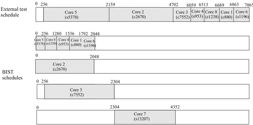
considers only the resource (RC) and core (CC) constraints. As shown in Figure 2.9, the example SOC test system S1 consists of eight different SOC cores (namely c880, c2670,

c7552, s953, s5378, s1196, s13207 and s1238 in Table 2.1). All the cores, except core s13207, share the same external-test bus. Cores c2670, c7552 and s13207 have their own dedicated BIST logic. As shown in Figure 2.9, cores c880, s953, s5378, s1196 and s1238 share the same built-in-self-test (BIST) logic. In Figure 2.9, the testing cycle times for the external-test and BIST of each core are shown within parentheses, and the power dissipation (either on external-test or BIST) of each core is shown within brackets. In this chapter, according to the industry practice, it is assumed that the power dissipation on BIST is 10 times of that on the external-test. In this example of SOC test system, the maximum allowed power dissipation (Pmax) is assumed to be 750 mW.

Figure 2.10 shows the best solution of SOC test schedule for the example system S1

considering only the resource (RC) and the core (CC) constraints. The optimal schedule is found to be 6809 clock cycles, which is the same as reported in [Iyengar 01b]. On finding the optimal solution, the developed NN took only 1.07 CPU seconds, compared to 3 CPU seconds by the mixed integer linear programming method (MILP) in [Iyengar 01b]. Figure 2.11 shows the optimal test schedule for the example system S1 by adding the precedence

(33)

So far, we have not considered the power constraint PoC in the example system S1.

Figure 2.12 shows a feasible test schedule first found by the developed NN for the example system S1, with the consideration of all the constraints (RC, CC, PC, and PoC constraints).

Due to the added power constraint PoC, the completion time of the test schedule is 8192 clock cycles, which is larger than the completion time of the example shown in Figure 2.11. Notice that, in Figure 2.12, idle time exists in the feasible test schedule, which can be further optimized. The idle time gaps in the feasible test schedule may occur when the solution space is very big. The developed NN eliminates the idle time gaps during its optimization process and searches for globally optimal test solution. Figure 2.13 shows the optimal test schedule generated by the developed NN for the example test system S1. As shown in Figure

2.13, eliminating the idle time by the developed NN, the completion time of the optimal test schedule for system S1 is found to be 7065 clock cycles which is much better than the

original result in Figure 2.12.

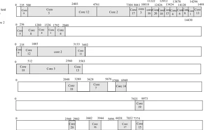
Figure 2.14 shows the second example of the SOC test system S2 with thirteen cores,

one external-test bus and four BIST logics. Detailed data of the second example system S2

are listed (as the first thirteen cores) in Table 2.2. As shown in Figure 2.14, three groups of cores share three BIST logics, and core 7 has its own dedicated BIST. Except for cores 7 and 11, all the other cores are accessible to the external-test bus, as shown in Figure 2.14. The maximum allowed power dissipation for the example system S2 is assumed to be 750 mW.

Figure 2.15 shows the optimal test schedule generated by the developed method for the example of SOC system S2. As shown in Figure 2.15, the optimal test schedule is 10713

clock cycles. The optimal SOC test solution for the developed NN takes 26.61 CPU seconds for the example system S2, compared to 142 CPU seconds of a similar system with 12 cores

by the MILP method reported earlier in [Iyengar 01b].

(34)

S3 is considered as a large size SOC system, and S3 consists of twenty cores, one external-test

bus and six BIST logics, as shown in Figure 2.16. Detailed data of all the twenty cores of the testing system S3 are shown in Table 2.2 (cores 1 to 20). In the SOC system S3, five groups

of cores share five BIST logics, and core 19 has its own dedicated BIST, as shown in Figure 2.16. In the test system S3, except for cores 7, 11, 14, 18 and 19, all the other cores are

accessible to the external-test bus. Figure 2.17 shows the optimal SOC test solution of 14,990 clock cycles generated by the developed NN for the example system S3. Notice that,

in Figure 2.17, the optimal SOC test schedule found by the NN is the optimal result and the completion time is equivalent to the lower bound of the test system S3. By using the

developed method, the computation time for the large size system S3 is 750 CPU seconds

(using MATLAB® program).

Table 2.3 shows the summary and comparison of the computation results generated by the developed NN method (after twenty runs of searching iterations) for the example systems S1, S2 and S3 with different constraints. As shown in Table 2.3, each example system

is tested with four combinations of constraints: (i) resource constraint and core constraint, (ii) resource constraint, core constraint and precedence constraint, (iii) resource constraint, core constraint, precedence constraint, and power constraint that considers only BIST resource, and (iv) similar to (iii) but considering both the external-test and BISTs. As shown in Table 2.3, for twenty runs, the proposed NN finds nine out of twelve testing problems with the best solutions (the lower bound). The examples and Table 2.3 show that the proposed NN method is not only capable of solving the large size SOC test problems but also able to find the optimal solutions within reasonable time. Except for some very large size SOC problems (20 cores), the proposed method generates the optimal SOC test solutions within efficient computing time, as shown in Table 2.3.

2.6 Summary

(35)

(36)

Figure 2.1 Picture of an example System-on-a-Chip (SOC) design and testing [Pino 96]

BIST BIST

BIST

Core 1 Core 2 Core 6

Core 3 Core 4

Core 5 External

test bus

(37)

x

I

x

1

y

J

x

i

y

1

y

j

w

1 j

a

0 1

w

1 J

w

i 1

w

i j

w

i J

w

I 1 _w I j

w

I J

a

0 j

a

0 J

w

1 1

Input units Output units

Figure 2.3 A single-layer neural network

Σ

w_{1 j}

w_{2 j}

w_{I j}

S_j

y_j f S( )_j

a_{0 j}

x₁

x₂

x_I

(38)

25 Cor e c ons tra int (C C) bl oc k un it Re sour ce c onst ra int (RC) bl oc k un it Pr ec ede nc e c on str aint (P C ) bl oc k u nit Input w a w c w b w d Σ Σ Σ Σ Σ ST u 13 () B NN 2 NN 2 ST 11 ST u 11₍₎ w a w c w b w d ST u 12 () B NN1 NN 1 ST u 11₍₎ w a w c w b w d ST u MI () ST MI B NN l NN l ST M-1 ,I ST u M-1 ,I() ST 11 ST 12 ST 13 w a w c w b w d Σ ST u 31 () B NN2 NN 2 ST 11 ST u 11₍₎ w a w c w b w d ST u 21 () B NN 1 NN 1 ST u 11 () w a w c w b w d ST u MI () ST MI B NNl NN l ST M, I-1 ST u M, I-1 () ST 11 ST 21 ST 31 w a w c w b w d Σ Σ Σ Σ Σ B NN2 NN 2 ST 12 ST u 12 () w a w c w b w d B NN 1 NN 1 w a w c w b w d ST MI B NNl NN l ST M-1 ,I ST 11 ST 21 ST 21 ST U 11 () ST U 21 () ST U 21 () ST U M-1 ,I() ST U MI () ST u 11 () ST u 21 () ST U 21₍₎ ST u 21₍₎ ST U M-1, I() ST u M-1 ,I() ST U MI () ST u MI () ST U 11₍₎ ST U 21 () ST u’ 21 () ST u’ 21 () ST u’ 11₍₎ ST u’ MI () ST u’ M-1 ,I() [, , ] ST t P 22 2 [, , ] ST t P MM M a 21 a M1 a 1j a 1J a 2j a Mj a 2J a MJ a 11 NP j NP J NP 1 w 1j w 1J w 21 w 2j w 2J w M1 w Mj w MJ w 11 P ma x P max P ma x [, , ] ST t P 11 1 [, , ] ST t P MM M a 21 a M1 a 1j a 1J a 2j a Mj a 2J a MJ a 11 NP j NP J NP 1 w 1j w 1J w 21 w 2j w 2J w M1 w Mj w MJ w 11 P ma x P max P ma x [, , ] ST t P 11 1 Σ Σ Σ Σ Σ ST u’ 21₍₎ ST u’ 21 () ST u’ 11 () ST u’ MI () ST u’ M-1 ,I() Σ Σ Σ Σ Po w er c on str aint (P oC) b loc k uni t [, , ] ST t P 22 2 [, , ] ST t P ii i Fi gu

re 2.5 Th

e proposed

neural netwo

(39)

ST e x ST f y NN l w a w c w b w d B

N N l

ST

f y(0)

ST

e x(0) STe x( )U

ST u

e x( )

ST U

f y( )

ST u

f y( )

Output Input

Figure 2.6 The proposed structure of a general constraint (PC, RC, CC) unit

Input node Output node

[ST t ,P ]

2

,

2 2

[ST ,t ,P ]

M M M

[ST t P, , ]

i i i

a

2 1 a_{M 1}

a 1 j a 1 J a 2 j a M j a 2 J a M J a 1 1 NP j NP J NP 1 w 1 j w 1 J w 2 1 w 2 j w 2 J w M 1 w M j w M J w 1 1 P

m a x

P

m a x

P

m a x

Input

[ST t, ,P ]

1 1 1

Output ST u

i( )

Power constraint (PoC) block unit

(40)

Feasible solution

Best feasible solution

Random search

(To improve a feasible solution)

“Idle time elimination” Algorithm The proposed

neural network

Can the idle time be shorten? No

Yes

No Yes

No Initial input

(41)

Table 2.1 Test data of the cores for the SOC system S1 [Iyengar 01b]

Circuit (core)

Core index

i

Number of scan element, s

Number of scan patterns

Number of scan cycles

Power (P_i, mW)

(External Test)

Number of BIST patterns

Number of BIST cycles

Power

(P_i, mW)

(BIST)

c880 1 60 26 134 5 4096 256 54

c2670 2 233 158 2543 16 32758 2048 159

c7552 3 207 96 1357 45 32768 2048 453

s953 4 52 90 454 6 4096 256 57

s5378 5 228 118 1903 32 4096 256 324

s1196 6 32 80 242 7 4096 256 72

s13207 7 790 - - - 32768 2048 592

s1238 8 32 58 176 7 16384 1024 75

External test bus

c2670 c7552 _s13207

c880

s953 s5378 s1196

s1238

BIST

BIST BIST BIST

(2543, 2048) [16, 159]

(1357, 2048)

[45, 453] (-, 2408) [-, 592]

(454, 256) [6,57]

(134, 256) [5, 54]

(1903, 256)

[32, 324] (242, 256) [7, 72]

(176, 1024) [7, 75]

( ) : (Testing time cycle for external test, Testing cycle for BIST test )

[ ] : [Power consumed while tested on external test, Power consumed while tested on BIST]

(42)

0 0 0 0 0 Core 5 (s5378) Core 4 (s953) Core 3

(c7552) Core 6(s1196) Core 2(c2670)

Core 1 (c880) Core 1 (c880) Core 2 (c2670) Core 6 (s1196) Core 3 (c7552) Core 4 (s953) Core 7 (s13207) Core 5 (s5378) 2048 2048 2048 Core 8 (s1238) Core 8 (s1238)

176 2079 2213 3570 3812 4266 6809

176 1200 1456 1712 1968 2213 2469

External test schedule

BIST schedules

Figure 2.10 The best result of test schedule for the system S1 with only RC and CC constraints

(Computing time = 1.07 CPU sec< 3 CPU sec by using MILP [Iyengar 01b])

External test schedule BIST schedules 0 256 0 0 0 0 Core 5 (s5378) Core 4 (s953) Core 3 (c7552) Core 2 (c2670) Core 6 (s1196) Core 1 (c880) Core 1 (c880) Core 2 (c2670) Core 6 (s1196) Core 3 (c7552) Core 4 (s953) Core 7 (s13207) Core 5 (s5378)

2159 4702 5156 5332 5466 5708 7065

256 512 1536 1792 2048

2048 2048 2048 Core 8 (s1238) Core 8 (s1238)

Figure 2.11 The best result of test schedule for the system S1 with RC, CC and PC constraints

(43)

External test schedule BIST schedules 0 0 0 0 0 2048 256 1280

2159 4702 6059 6513 6689 6863 7065

256 1536 1792 2048

256 2304

6144 8192

Core 5

(s5378) Core 4(s953)

Core 3 (c7552) Core 2 (c2670) Core 6 (s1196) Core 1 (c880) Core 1 (c880) Core 2 (c2670) Core 6 (s1196) Core 3 (c7552) Core 4 (s953) Core 7 (s13207) Core 5 (s5378)Core 8(s1238)

Core 8 (s1238)

Figure 2.12 A feasible test schedule for the system S1 with all the constraints RC, CC, PC, and PoC

(The feasible test schedule has some idle time that should be eleminated) (The completion time = 8192 clock cycles)

External test schedule BIST schedules 0 0 0 0 0 2048 256 1280

2159 4702 6059 6513 6689 6863 7065

256 1536 1792 2048

256 2304 2304 4352 Core 7 (s13207) Core 3 (c7552) Core 2 (c2670) Core 5

(s5378)Core 8(s1238)Core 4(s953) Core 1_(c880) Core 6_(s1196)

Core 5

(s5378) Core 2(c2670) Core 3(c7552)

Core 4

(s953) Core 8(s1238) Core 1(c880)

Core 6 (s1196)

Figure 2.13 The best result of test schedule for the system S1 with all the constraints RC, CC,

(44)

External test bus

BIST

BIST (2543, 2048)

[16, 159] _{(1357, 2048)}

[45, 453] (-, 2408) [-, 592] (454, 256) [6,57] (134, 256) [5, 54] (1903, 256)

[32, 324] (242, 256) [7, 72]

(176, 1024) [7, 75] Core 1

Core 2

Core 3

Core 7

Core 8

Core 9 Core 10

(265, 235) [18, 180] (2358, 850) [9, 86] Core 11 Core 12 Core 13 (-, 469) [-, 236] (486, 512) [15, 153] (560, 1023) [31, 315] BIST BIST

Figure 2.14 The second example of the SOC system S2 with 13 cores

Table 2.2 Test data of the cores for the SOC system S2and S3

External test BIST External test BIST

Core index

(i) time (Testing t_im) Power (mW) Pim time (Testing t_im) P_imPower (mW)

Core index

(i) time (Testing t_im) P_imPower (mW) time (Testing t_im) Power P_im

(mW)

1 134 5 256 54 11 - - 469 236

2 2543 16 2048 159 12 2358 9 850 86

3 1357 45 2048 453 13 560 31 1023 315

4 454 6 256 57 14 - - 1240 412

5 1903 32 256 324 15 512 41 342 415

6 242 7 256 72 16 1204 8 342 78

7 - - 2048 592 17 1357 16 342 162

8 176 7 1024 75 18 - - 1240 95

9 265 18 235 180 19 - - 2048 365

(45)

External test schedule

BIST schedules

0

Core 5 Core 2 Core₃ Core₄ Core 6 Core 1

Core 1

Core 2 Core 6

Core 3

Core 4 Core

5 Core 8

Core 8 Core

9 Core 10

Core

12 Core ₁₃

Core

9 Core 12 Core ₁₁

Core

10 Core 13

235 500 2403 4946 6303 6479 8837 9291 9777 10019 10153 10713

256 1280 1536 1792 2048

235 2283 3133 3602

277 2325 3860

7713 9761

2837

PC and PoC

(46)

External test bus

BIST (2543, 2048)

[16, 159] (1357, 2048)_{[45, 453]}

(1204, 342) [8, 78] (454, 256) [6,57] (134, 256) [5, 54] (1903, 256) [32, 324] (242, 256) [7, 72] (176, 1024) [7, 75] Core 1

Core 2 Core 3

Core 8

Core 9 Core 10

(265, 235) [18, 180] (2358, 850) [9, 86] Core 11 Core 12 Core 13 (-, 469) [-, 236] (486, 512) [15, 153] (560, 1023) [31, 315] BIST BIST Core 14 Core 15

Core 20 (1357, 342) [16, 162] (512, 342) [41, 415] (-, 2408) [-, 592] Core 7 (-, 1240) [-, 412] (1204, 342) [8, 85] (-, 2408) [-, 365] BIST Core 18 (-, 1240) [-, 95] BIST BIST

(47)

External test schedule BIST schedules 0 0 0 0 0 Core

5 Core ₄

Core 2

Core 6 Core 1

Core 1 Core 2 Core 6 Core 3 Core 4 Core

5 Core 8

Core 8

Core

9 Core 12 Core 10

Core 13

Core

9 Core ₁₂ Core ₁₁

Core

10 Core 13

0 0 Core 7 Core 15 Core 17 Core 18 Core 19 Core 20 Core 15 Core 16 Core 17 Core 20 256 512

1280 1536 1792 2048

235 1085 _{3133 3602}

2560 3583

2048 3288 3628 _{5676 5700 6940}

7925 9973

core 2

2560 2902 3602 3944 5696 6038 7032 7374

235 500 2403 4761 7304 8661 10018

11222 12426

12912

134241387814120 14296

14430 14990 core

3 core 16

PC, and PoC

(48)

Table 2.3 The SOC test scheduling solutions from the proposed NN after 20 runs

Computational time (second) Problems Lower

bound Solbest ∆Sol%

Solavg

Taverage Tmax Tmi

8 cores with 2 constraints 6809 6809 0 - 1.07 3.68 0.27

8 cores with 4 constraints (BIST) 7065 8192 15.95 8192 65.48 94.31 50.92

8 cores with 4 constraints (ALL) 7065 8547 20.98 8619 357.64 440.94 294.45

13 cores with 4 constraints (BIST) 10713 10713 0 10859 26.61 95.8 2.5

13 cores with 4 constraints (ALL) 10713 10713 0 10889 326 1759.3 34.3

20 cores with 4 constraints (BIST) 14990 14990 0 15178 750 2551 141

20 cores with 4 constraints (ALL)**_{14990 15369 2.53} _{20900 -} _-

**_{run only one time.}

Lower bound: optimal value from ILP method [Iyengar 01b]

Solbest: value of the best solution found by the proposed NN out of 20 runs.

∆Sol%: = ((Solbest - Opt)/Opt)*100 if the optimum is known,

= ((Solbest - LB)/LB)*100 otherwise.

Solavg : average solution value over 20 runs or nothing if all runs gave the optimum value.

Taverage: average computing time, in seconds.

Tmax: maximum computing time for one run, in seconds

(49)

CHAPTER 3 DEVELOPING MAXIMUM NEURAL NETWORK TO SOLVE TEST

RESOURCE ALLOCATION AND TESTING TIME MINIMIZATION

FOR THE SYSTEM-ON-A-CHIP (SOC)

This chapter presents a maximum neural network to minimize the testing time and optimize resource allocation for a System-on-a-Chip (SOC) test system design. By determining the allocation of cores to test access mechanism (TAM) and the TAMs width in a SOC system, the testing time can be reduced. Constraints considered in the SOC test system design include the following: (i) SOC cores allocation (ii) TAMs width selection, and (iii) power consumption. The objective of this investigation is to achieve the optimal testing time for a SOC test system design with the optimal core allocation and TAMs width selection within a reasonable computation time.

3.1 Introduction

(50)

When a SOC system designer/integrator gets cores from a core provider, he/she encounters two major tasks in solving the SOC test problems. The first task is how to design a test access mechanism (TAMs) and the second task is how to determine the test schedules for a SOC system to minimize the time-to-market [Iyengar 01b]. TAMs must be designed to transport pre-computed tests from system I/Os to core I/Os. In recent years, several new TAMs have been proposed such as Test Bus [Varma 98], and TESTRAIL [Marinissen 98]. Test scheduling determines the order in which the various cores are tested and what testing resources are used for SOC testing subject to variety of hardware, sequence and capacity constraints.

Figure 3.1 shows an example of a core-based SOC with two TAMs [Chakrabarty 00a]. The system has 10 cores: 2 combinational cores and 8 cores with internal scan. These cores must be allocated to each TAM and the TAM partition is considered such that the overall testing time is minimized. The SOC testing design with resource allocation problems are NP-complete [Chakrabarty 00a]. When a SOC system is small (less than 10 cores), using traditional methods such as integer linear programming (ILP) or a heuristic approach can solve the problems easily. However, when the system becomes more complex, using traditional methods may not be efficient or effective because the optimal solution is difficult to achieve and the computation time is long.