Specification and Estimation of Economic Models of Asset Prices

(1)

ROBERTS, MATTHEW CHRISTOPHER. Speciﬁcation and Estimation of

Econo-metric Models of Asset Prices. (Under the direction of Barry K. Goodwin and Alastair

Hall.)

The three essays of this thesis research model selection and estimation issues in

ﬁnancial econometrics. Special attention is given to comparing various approaches

used previously in the literature and attempting to compare their out-of-sample

per-formance.

Chapter two explores the value of modelling the deterministic seasonal component

of volatility and alternate conditional distributions for the soybean futures market.

The simultaneous modelling of deterministic seasonal volatility and conditional

het-eroscedasticity provides for much more precise predictions of observed options prices.

Likewise, for the purposes of volatility forecasting, ﬂexible conditional distribution

modelling does not seem to beneﬁt volatility forecasting.

Chapter three compares the performance of continuous-time and discrete-time

models of time-varying volatility, speciﬁcally stochastic volatility and GARCH

pro-cesses. These models are again applied to the soybean futures markets. The results

conclude that signiﬁcant tradeoﬀs must be made in using continuous-time models

in option price prediction. The ﬂexibility of GARCH processes when applied to

discretely-sampled data allows more accurate and precise prediction and simulation

of volatility processes.

Chapter four compares the performance of three alternative models for

stochas-tic discount factor estimation. In doing so, previously overlooked weaknesses of the

approaches are revealed. Contrary to previous research, this chapter ﬁnds less

sup-port for two-factor and nonlinear speciﬁcations. Most signiﬁcantly, in out-of-sample

pricing, the non-negativity restriction previously tested in Bansal and Viswanathan

(1993) was found to possibly oﬀer some beneﬁt, as economic theory would suggest,

(2)

by

MATTHEW C. ROBERTS

A thesis submitted to the Graduate Faculty of

North Carolina State University in partial fulﬁllment of the requirements for the Degree of

Doctor of Philosophy

ECONOMICS

RALEIGH 2001

APPROVED BY:

Walter N. Thurman Duncan Holthausen

Barry K. Goodwin Committee Co-Chairman

Alastair Hall

(3)

(4)

Biography

Matthew C. Roberts was born 9 December, 1971 to William H. and Carolyn Roberts

of Bolivar, Missouri. He is the 5th of 6 children, and remained in Bolivar for the

duration of his primary and secondary schooling.

The author’s exposure to economics began early. By age ﬁve, he had his own desk

at Bill Roberts Chevrolet, his father’s auto dealership, in spite of the lack of evidence

of his ever having accomplished any real work.

Matthew’s ﬁrst exposure to ‘real’ economics occurred at a summer camp sponsored

by Drury College during the summer following the seventh grade. A course he enrolled

in, taught by a professor whose name has been consigned to mists of history, was

an introduction to macroeconomics. The instructor was very talented in explaining

the issues of economics, and the course culminated in teams presenting solutions to

various macroeconomic problems of the day.

The High School years were primarily spent pursuing other avenues of interest. A

required Economics course during 11th grade was not only utterly devoid of content,

but mutual, open antagonism between Matthew and the instructor was only stopped

by the direct intervention of the superintendent of schools (as well as Matthew’s

mother, it must be added.) Let the annals of history reﬂect that whatever

achieve-ments, awards, or infamy Matthew may accrue during his career in Economics, they

have absolutely nothing to do with his 11th grade Economics course, whose

instruc-tor, having not taught anything approaching economics, obviously had absolutely no

bearing on the economic education of the author.

Following the 11th grade year, Matthew enrolled in college summer courses at

the nearby Southwest Missouri State University. One of the courses was Principles

of Macroeconomics. Although a Keynesian, the instructor nonetheless did much for

Matthew’s burgeoning interest in the ﬁeld.

(5)

University of Missouri at Columbia for one year, and then transferred to William

Jewell College in Liberty, Missouri. At William Jewell, Matthew majored in

Eco-nomics, under the direction of Dr. Michael Cook. During his Junior year, Matthew

met his future wife, Mardi. Her major required one year to be spent studying in a

German-speaking country. She had made arrangements to spend her senior year in

Vienna, Austria. Soon after the beginning of their senior year, Matthew decided that

international study might be an attractive option, and arranged to spend the second

semester of his senior year in Vienna, Austria, too.

After graduation, Matthew and Mardi married and remained in Vienna seeking

work. Matthew found employment with ACS Acquisition Services, and Mardi was

employed by Business Central Europe, a daughter publication of The Economist. Six

months later, Matthew moved to CA Global Futures, the futures and derivatives

brokerage subsidiary of Creditanstalt Bankverein. They remained in those positions

until May 1996, when they left to return to the United States, at which point Matthew

began his graduate studies at North Carolina State University, culminating with this

dissertation.

Matthew is now an Assistant Professor in the Department of Agricultural,

Envi-ronmental, and Development Economics at The Ohio State University in Columbus,

(6)

Acknowledgements

This dissertation would have never been possible without the love, understanding and

support of my wife, Mardi; to her I owe the greatest debt. Without the examples

of hard work, dedication, and the value of education set by my parents, Bill and

Carolyn, I would’ve never been been capable of beginning this work.

The mentoring of Barry Goodwin has likewise been invaluable in my graduate

studies. My professional career will be forever improved by the time and energy he

devoted to me as a graduate student. I would also like to thank Paul Fackler for

all of his help throughout my graduate studies. The eﬀorts of Alastair Hall are also

gratefully acknowledged; his comments, advice, and eﬀort immeasurably improved

this dissertation. Finally, I would like to thank John Dodrill, Aaron Hegde, Charles

Fulcher, and John Deal for their friendship and support throughout my graduate

(7)

List of Tables

2.1 Futures Prices Sample Statistics . . . 25

2.2 GARCH Estimates . . . 26

2.3 t-GARCH(1,1) Estimates . . . . 27

2.4 MIXGARCH(1,1) Estimates . . . 28

2.5 Mixture Distribution Bootstrap Test Results . . . 29

2.6 GARCH Option RMSEs . . . 29

2.7 GARCH Option Mean Diﬀerences . . . 30

2.8 t-GARCH Option RMSEs . . . . 31

2.9 t-GARCH Option Mean Diﬀerences . . . . 32

2.10 MIXGARCH Option RMSEs . . . 33

2.11 MIXGARCH Option Mean Diﬀerences . . . 34

3.1 SNP Model-ﬁtting Results . . . 62

3.2 EMM Model-ﬁtting Results . . . 63

3.3 SV and GARCH Option RMSEs . . . 64

3.4 SV and GARCH Option MADs . . . 65

3.5 SV and GARCH Option Mean Error . . . 66

4.1 SDF Estimation Results . . . 92

4.2 Model Diagnostics: Correlation and Out of Sample Results . . . 93

B.1 Simulation Parameter Values . . . 115

B.2 Simulation Results . . . 115

(10)

List of Figures

2.1 Soybean Futures Nominal Prices . . . 35

2.2 Soybean Futures Log-Change in Prices . . . 35

2.3 Seasonal trends in GARCH . . . 36

2.4 Gaussian GARCH Residuals . . . 36

2.5 Seasonal trends int-GARCH . . . . 37

2.6 Estimated t-GARCH distributions . . . . 37

2.7 t-GARCH Residuals . . . 38

2.8 Seasonal trends in MIXGARCH . . . 38

2.9 Estimated MIXGARCH distributions . . . 39

2.10 MIXGARCH Residuals . . . 39

3.1 Estimated SNP Distribution . . . 67

3.2 EMM Moment Condition Standard Errors . . . 67

4.1 State Factor Returns . . . 94

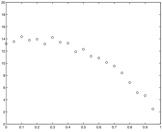
4.2 Smoothing Parameter Cross Validation: One Factor . . . 94

4.3 Smoothing Parameter Cross Validation: Two Factor . . . 95

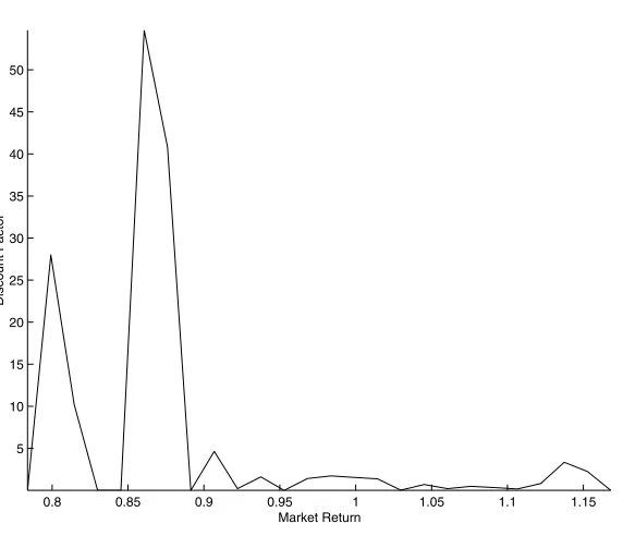
4.4 One Factor, Linear SDF . . . 95

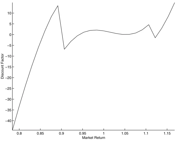
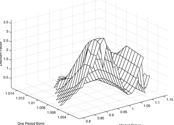
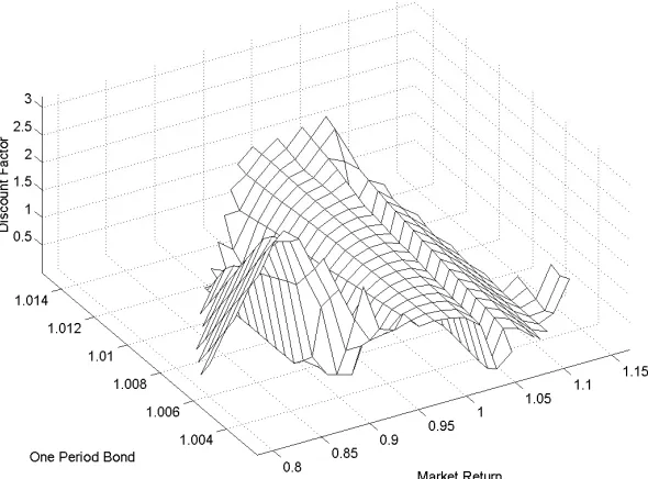
4.5 One Factor, Nonlinear, Unrestricted NN SDF . . . 96

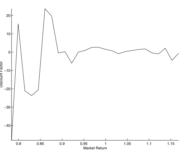
4.6 One Factor, Nonlinear, Unrestricted POLY SDF . . . 96

4.7 One Factor, Unrestricted Smoothing SDF withλ = 0 . . . 97

4.8 One Factor, Unrestricted Smoothing SDF withλ = 0.95 . . . 97

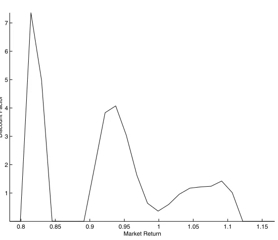
4.9 One Factor, Nonlinear, Nonnegative NN SDF . . . 98

4.10 One Factor, Nonlinear, Nonnegative POLY SDF . . . 98

4.11 One Factor, Nonnegative Smoothing SDF with λ∗ = 0 . . . 99

4.12 One Factor, Nonnegative Smoothing SDF with λ∗ = 0.95 . . . 99

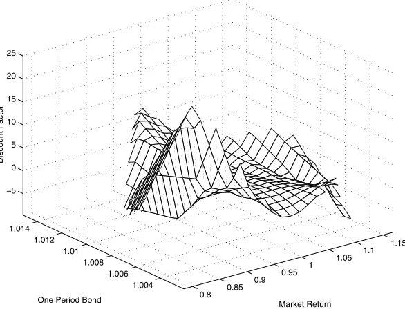
4.13 Two Factor, Linear SDF . . . 100

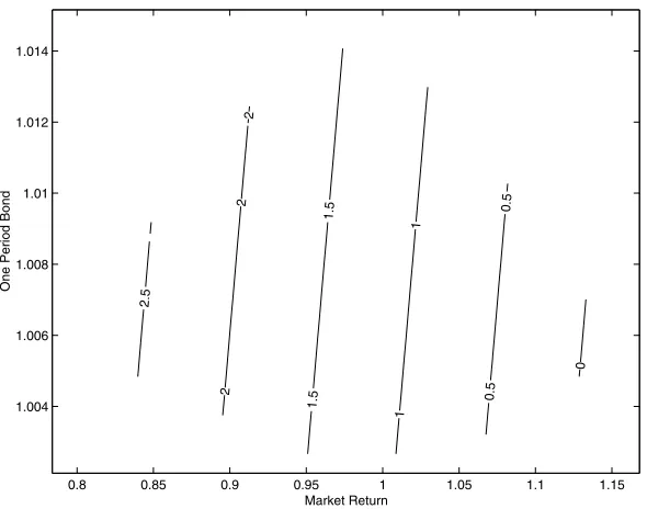
4.14 Two Factor, Linear SDF – Contour . . . 100

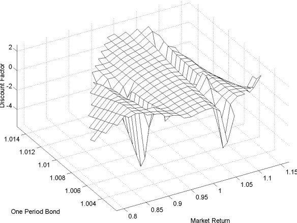
4.15 Two Factor, Nonlinear, Unrestricted NN SDF . . . 101

4.16 Two Factor, Nonlinear, Unrestricted POLY SDF . . . 101

4.17 Two Factor, Unrestricted Smoothing SDF with λ∗ = 0 . . . 102

4.18 Two Factor, Unrestricted Smoothing SDF with λ∗ = 0.95 . . . 102

4.19 Two Factor, Nonlinear, Nonnegative NN SDF . . . 103

(11)

4.21 Two Factor, Nonnegative Smoothing SDF with λ∗ = 0 . . . 104

4.22 Two Factor, Nonnegative Smoothing SDF with λ∗ = 0.95 . . . 104

B.1 One Factor, Linear Simulation Plots . . . 117

B.2 Two Factor Linear Diﬀerence Plot . . . 117

B.3 One Factor, Nonlinear Neural Network Simulation Plots . . . 118

B.4 One Factor, Nonlinear Polynomial Simulation Plots . . . 118

B.5 Two Factor Nonlinear Diﬀerence Plot, NN vs. NN . . . 119

B.6 Two Factor Nonlinear Diﬀerence Plot, NN vs. POLY . . . 119

B.7 Two Factor Nonlinear Diﬀerence Plot, NN vs. SM . . . 120

B.8 Two Factor Nonlinear Diﬀerence Plot, POLY vs. NN . . . 120

B.9 Two Factor Nonlinear Diﬀerence Plot, POLY vs. POLY . . . 121

(12)

Chapter 1 Introduction

Modelling the price behavior of ﬁnancial instruments has been the impetus for

much of the development of modern ﬁnancial econometrics. Early on, these endeavors

were viewed by many as alchemy: a quest to ﬁnd some lucrative, hidden structure

buried deep beneath the erratic movements of prices. As the ‘Eﬃcient Markets’ and

‘Rational Expectations’ paradigms overtook economics, the study of price processes

became less concerned with price changes themselves, and more concerned with the

stochastic processes that govern them (Fama (1965) and Mandelbrot (1963)).

In this vein, this thesis proposes to investigate three speciﬁc stochastic processes

and examine the results and their implications for ﬁnancial economics. The

pro-posed processes are the formation of options prices in the presence of conditional

heteroscedasticity, options pricing in the presence of stochastic volatility, and the

stochastic discount factor estimation methods.

Commodity prices tend to have seasonal supply and demand characteristics.

Lit-tle prior work has examined the size or importance of these deterministic patterns

and their eﬀects on the conditional distribution of prices. Chapter two uses

previ-ously proposed methods to explicitly capture these eﬀects in an econometric model of

(13)

demonstrated in the ability of this model to predict options prices. The seasonal

mod-elling of volatility greatly reduces prediction error. Flexible conditional distributions,

however, are of little additional value.

Chapter three investigates the ability of continuous-time stochastic volatility

mod-els to represent the commodity futures markets. Continuous-time modmod-els are

fre-quently preferred in the ﬁnance literature for their tractability in asset-pricing

appli-cations. The question of the cost of this preference has not been addressed. Chapter

three compares the performance of the two models in their abilities to predict the

prices of options on CBOT futures. The results indicate that continuous-time

stochas-tic volatility models may have serious disadvantages in comparison to discrete-time

conditional heteroscedasticity models.

Chapter four compares the performance of three alternative models for

stochas-tic discount factor estimation. In doing so, previously overlooked weaknesses of the

approaches are revealed. Contrary to previous research, this chapter ﬁnds less

sup-port for two-factor and nonlinear speciﬁcations. Most signiﬁcantly, in out-of-sample

pricing, the non-negativity restriction previously tested in Bansal and Viswanathan

(1993) was found to possibly oﬀer some beneﬁt, as economic theory would suggest,

but contrary to the ﬁndings in Bansal and Viswanathan.

(14)

Chapter 2 Options Pricing: Mixture

Distributions and Seasonality

2.1 Introduction

Derivatives contracts have existed for millennia. Aristotle referred to an option

contract when he wrote about “a ﬁnancial device which involves a principle of

univer-sal application” in Book I ofPolitics. Similarly, the vagaries of weather and pestilence

have plagued farmers since the beginning of time. And although recent decades have

seen an explosion of derivative products, both for ﬁnancial and commodity assets,

little research has been conducted on the speciﬁc interaction of derivative prices and

the unique characteristics of commodities. This paper explores one such

character-istic, the tendency for the volatility of commodity prices to systematically vary over

the course of the year, and examines the eﬀects of this behavior on an options pricing

model applied to Chicago Board of Trade soybean futures.

There existed no rational pricing method for even simple options until Black and

Scholes’ pricing model was developed. This, in combination with its no-arbitrage

(15)

ex-plosion of new derivative contracts. And although the genesis of derivative products

as we know them today comes almost entirely from commodity markets, most

pre-vious research has focused on ﬁnancial derivatives. Sound reasons existed for this

emphasis. Financial instruments were immune to production uncertainty and

de-mand should be constant, or aﬀected only by easily observable characteristics, such

as volatility and the prevailing interest rate environment. Financial instruments also

oﬀer the advantage of highly liquid and transparent spot markets. The markets for

ﬁnancial instruments were simply easier to model.

As users’ sophistication grew, demand for similarly complex products across other

markets likewise grew. Currently, there is little distinction between markets when it

comes to the variety of instruments available. Instruments introduced on short-term

interest rates will quickly spread to commodities if demand exists.

However, the transition from currencies to interest rates is much smoother than

that to commodities, especially agricultural products. The production cycle of

agri-cultural commodities, combined with the important role of climate and weather,

pro-duce very distinctive behavior in commodity prices. Using observed options prices,

this paper demonstrates that the inclusion of systematic seasonal variation, as in

Fackler (1986), and ﬂexible conditional distributions in commodity price modelling

improves the ability of time-series models to predict options prices as a demonstration

of the improved forecasting of the volatility process.

This paper has seven sections. The second section explains the time-series models

used in this estimation. The third section discusses estimation of the futures price

model. The fourth section reviews the theory of options pricing, while the ﬁfth section

details the procedures used to estimate the options prices. The sixth section reports

(16)

2.2 Time Series Models

In order to explore the eﬀects of commodity-speciﬁc characteristics, a time-series

model is ﬁrst speciﬁed. There are two competing families of time-varying volatility

models, autoregressive conditional heteroscedasticity (ARCH) and stochastic

volatil-ity (SV). The ARCH family was introduced by Engle (1982), and later, Bollerslev

(1986) introduced the Generalized ARCH (GARCH) model. In the ensuing years,

over 50 additional variants have been introduced, see Bollerslev (1999). ARCH

mod-els are discrete-time modmod-els which posit that variance is an unobserved, yet

determin-istic function of past variances and disturbances. The stochastic volatility literature

traces its roots to Clark (1973). Within the stochastic volatility literature, there are

two main sets of models, continuous-time and discrete-time. The discrete-time model

treats variance as an unobserved, stochastic process, typically exhibiting an AR(p)

process. The continuous-time model is cast in the form of multiple Brownian motion

processes, of which one typically represents prices, and another represents volatility.

Each of these models has come to dominate a particular application in the

lit-erature. The continuous-time stochastic volatility models dominate the theoretical

ﬁnance and derivatives-pricing literature. As one example of this phenomenon, the

recent, widely-used text on derivatives pricing by Wilmott (1998) has exactly one

equation for discrete-time processes in its 700+ pages. The absence of discrete-time

processes is understandable; derivatives pricing is primarily concerned with the

deriva-tion of closed-form, or as nearly as possible, soluderiva-tions to the various derivatives

prod-ucts available. This is a feat to which continuous-time processes, and the calculus

that governs them, are uniquely suited.

In the discrete-time literature, the ARCH class of models has come to dominate

empirical applications of time-varying volatility. ARCH models, having closed-form

likelihood functions, are much easier to estimate than discrete SV models, which lack

(17)

2.2.1 GARCH Models

A GARCH(1,1) model takes the form1

y_t = µ+_t (2.1)

_t =

h_tη_t (2.2)

h_t = ω+αh_t₋1+δ2_t₋1 (2.3)

where η_t is an i.i.d. innovation with a distribution having unit variance. In this

framework, E_t₋1(2_t) =ht. Bollerslev showed that the unconditional variance of the

GARCH process is ω/(1−α−δ).

A slightly modiﬁed version of this model was used by Myers and Hanson. In

their model, ω becomes a time-varying linear function, ω_t, though they only used an

indicator variable which proxies for the change in contract maturities.

2.2.2 Seasonal Volatility

The role of seasonality in price volatility is well-known. Fackler (1986) modelled

seasonal eﬀects in volatility by substituting a Fourier expansion for the intercept of

the GARCH volatility equation. Bollerslev and Ghysels (1996) suggested the periodic

GARCH formulation to allow seasonal variation in all of the variance parameters,

though they only utilized indicator variables in their study. Beller and Nofsinger

(1998) independently implemented a similar scheme, again using only indicator

vari-ables. A Fourier expansion is used in this study to estimate the seasonal eﬀects of

variance. The form is

ω_t =κ+

M

m=1

[φ_msin(2πmτ) +ψ_mcos(2πmτ)] 0≤τ ≤1 (2.4)

1_{GARCH(p,q) models, wherein variance is a linear function of a greater number of lags of past}

(18)

whereτ denotes the time of year of the observation, for example 1 January would be 1/365. The use of the Fourier form produces a simple and smooth approximation of

the seasonal variance eﬀects.2 _M _{denotes the order of the expansion, and is chosen}

by the researcher.

2.2.3 t

-GARCH

A large literature has grown up around the proper speciﬁcation of the conditional

distribution in GARCH models. Bollerslev (1987) ﬁrst used the student-t

distribu-tion in GARCH modelling to capture condidistribu-tional leptokurtosis in equity index prices,

calling it t-GARCH. Baillie and Myers (1991) and Hsieh (1989) among many have

conﬁrmed the non-normality of the conditional distribution. In order to

incorpo-rate a student-t distributed density into the GARCH model of equation (2.2), the

t-distribution must be modiﬁed so that its variance is a function only of h_t, and not of ν. Bollerslev (1987) used the standardizedt-distribution,

f_ν(t|h_t) = Γ

_ν_{+ 1}

2

Γ

_ν

2

₋1

((ν−2)h_t)−1/2

×1 +2_th−_t1(ν−2)−1−(ν+1)/2, ν >2 (2.5)

This standardized t-distribution has a mean and skewness of zero, and

Var(t|h_t) = h_t

E[4_t|h_t] = 3(ν−2)(ν−4)−1h2_t, ν >4

As is well known, as ν → ∞, the t distribution approaches normality, and as

ν → 4, the kurtosis of the t increases toward inﬁnity, producing the desired

’fat-tailed’ behavior.

(19)

2.2.4 Mixture Distributions

Studies such as Cornew, Town and Crowsen, (1984) and Hudson, Leuthold and

Sarassoro (1987) have found commodity price series to be skewed and, in the GARCH

framework, conditionally leptokurtic. To address the issues of leptokurtosis and

skew-ness, student-tand discrete mixtures of normal distributions are used. They are

simul-taneously very ﬂexible and tractable. Hsieh (1989) used discrete mixture distributions

to capture other anomalies in the conditional distributions, which I will abbreviate

the MIXGARCH model. Using arbitrarily many components, a mixture distribution

can arbitrarily closely approximate any other distribution of similar support. Further,

when using mixtures of normals, the moments of the mixture distribution are easily

obtained and have relatively simple closed-form solutions.

The density function of a mixture of k discrete distributions is

f_k∗(x; Θ) =

J

j=1

λ_jf_j(x;θ_j) 0≥λ_j ≥1 ∀j,

j

λ_j = 1 (2.6)

where λ_j is the weight of the jth distribution, f_j(x), and x are the random variates.

The log-likelihood function associated with a mixture distribution is then

LLF(x; Θ) =

N

i=1 ln

J

j=1

λ_jf_j(x_i;θ_j) (2.7)

When η, the conditional distribution of equation 2.2, is distributed as a discrete mixture of normals, the speciﬁcation also nests the standard Gaussian case. This

holds true as well for the student-t distribution, as it limits to the Gaussian case as

the distribution parameter goes to inﬁnity. However, the student-t and the mixture

distributions do not nest one another.

From (2.6) above, a mixture of two independent normal distributions has ﬁve

pa-rameters; a mixing parameter, two means and two standard deviations. The GARCH

conditional distribution (η) must be mean zero and unit variance. These two

(20)

variance and mixing parameters of the ﬁrst distribution are arbitrarily chosen to be

functions of the remaining parameters.

For two components, the actual likelihood function used is

LLF(x, θ) =

T

t=1 ln

λ1f

x_t

√

h_t;µ1, σ 2

1 + (1−λ1)f

x_t

√

h_t;µ2, σ 2

2 /ht (2.8)

wheref(x;µ, σ2_{) is the normal p.d.f. This distribution has ﬁve parameters –}_µ

1, µ2, σ1, σ2,

and λ, and two restrictions – that the mixture distribution be mean zero and unit

variance. Using these restrictions, µ2 and σ2 are eliminated from numerical

estima-tion.

2.3 Time Series Models: Estimation

The estimation of the futures models proceeds quite naturally from the

combina-tion of the pieces explained above. Three models are estimated, a Gaussian GARCH

model, a t-GARCH model, and a MIXGARCH model. Each of these models is

es-timated using a small number of explanatory variables in the variance. This section

discusses the data used in estimation, the details of estimating each of these models,

and the results obtained.

2.3.1 Futures Data

Futures prices were drawn from the Bridge Information Services Futures Price

Database. Chicago Board of Trade Soybean futures of November expiry from 1

Oc-tober 1990 through 25 OcOc-tober 1997 were used for a total of 1,768 observations.

November contracts exhibited the most liquid options market, and so were chosen

for the estimation. A univariate time-series was generated by using the November

futures contract closest to maturity on each day, except during November, when the

(21)

weeks of observations is common, as the combination of decreasing liquidity and the

eﬀects of physical deliveries tends to erratically aﬀect volatility.

Figure 2.1 plots the nominal prices of the futures data. Figure 2.2 plots the series

actually used in estimation, which is 100×ln(P_t/P_t₋1) of the futures data. Table 2.1

provides descriptive statistics for the log changes, as well as the results of Box-Pierce

(1970) Q-Tests for autocorrelation in the means and squares. Serial autocorrelation

exists, especially in the squared observations.

2.3.2 Estimation of GARCH models

These models are all estimated using maximum likelihood(ML). If the conditional

distribution is misspeciﬁed, ML estimates are consistent, but no longer eﬃcient.

Quasi-maximum likelihood standard errors are reported.3 _{All of the estimation and}

simulation is performed in MATLAB.

A switching parameter in the variance equation is also estimated. This is

con-structed as a dummy variable indicating the change in maturity of observed contract

prices. The reason for including this term is that one typically expects the variance

of futures contracts to be inversely proportional to the maturity of the contract itself,

a stylized fact known as the Samuelson Hypothesis. Using only one variable for all

of the contract rolls makes the implicit assumption that this eﬀect is similar for each

occurrence. The revised model is of the form

100×ln(P_t/P_t₋1) = µ+t (2.9)

_t =

h_tη_t

h_t = ω_t+αh_t₋1+δ2_t₋1 ω_t = κ+SI_t+

M

m=1

φ_msin(2mπτ) +ψ_mcos(2mπτ) 0≤τ ≤1

where I_t is an indicator variable which is one if the previous observation is of a

(22)

diﬀerent maturity date than the current observation, and zero otherwise.

One additional parameter is estimated; h1 is the estimated variance of the ﬁrst

time period. Often in GARCH estimation, the unconditional variance ω/(1−α−

δ) is used for the initial variance. Estimating h1 as a parameter tends to improve small-sample performance, though asymptotically there is no diﬀerence in the two

approaches.

2.3.3 Gaussian Results

Table 2.2 presents the results of the estimation. The estimates of the GARCH

parameters αand δ accord with prior estimations, both in size and signiﬁcance. The

switching parameter is of the expected sign, but is not signiﬁcant. The residuals

continue to display leptokurtosis, though no signiﬁcant skewness, and the Q-tests fail

to demonstrate any autocorrelation in the residuals or their squares through 10 lags.

The second set of results in the table include a ﬁrst order seasonal expansion, as

in equation 2.4 above. The addition of these two parameters is not only highly

sig-niﬁcant from a LR test perspective (test statistic of 72 vs. aχ2

2) but is also preferred

from a SC (Schwartz criteria) perspective. In addition, the inclusion of seasonality

reduced the kurtosis in residuals, and the switching parameter is now highly

signif-icant. Additionally, the value of α has decreased, as the Fourier expansion reduces

the dependence of the estimated variance of a given date on that of the prior date.

These results largely correspond with the ﬁndings of Fackler (1986). Although he

found three orders of seasonality to be preferable, in all other respects the results are

similar.

Including a second order of seasonality adds only marginal beneﬁt. LR tests do not

support the signiﬁcance of the additional parameters, and the Akaike informantion

criteria (AIC) and Schwartz information criteria (SC) fall. The patterns established

(23)

falls further, though kurtosis is basically unchanged.

Figure 2.3 plots the unconditional expectation of the daily variance (EDV) of

the ﬁrst and second order seasonal models. In order to take into account the

au-toregressive nature of the process and the discontinuity introduced by the

switch-ing variable, ω_t is computed over the calendar year, t = 1. . .365. The process

EDV_t = ω_t+ (α+δ)·EDV_t₋1 is run until the EDV estimates converge. The cause

of the relative lack of improvement from adding the second order of seasonality is

apparent from the similarity of the two curves.

Gaussian estimation results demonstrate the importance of conditionally

het-eroscedastic models as well as the inclusion of seasonality in GARCH estimation. For

the model used here, one order of seasonality is the best balance between parsimony

and ﬁt. The residuals of the one-order model are plotted in ﬁgure 2.4. Comparing this

ﬁgure to 2.2 conﬁrms the decrease in autocorrelation revealed by the Q-Test results

above.

2.3.4 t

-GARCH Results

The estimation of the t-GARCH model proceeds very similarly to the Gaussian

GARCH model. The ν parameter of the distribution is actually estimated as 1/ν so

that the Gaussian case may be represented by 1/ν = 0. This eases estimation, as

the parameter is bounded on [0,0.5]. However, because the naturally desirable null

hypothesis of 1/ν = 0 lies at the boundary of the parameter’s domain, testing still

cannot be performed using standard tests. As in the Gaussian case above, h1 and a

switching parameter are also estimated.

Table 2.3 reports the results of the t-GARCH estimation. Omitting seasonality,

the estimation results are very similar to those reported for the Gaussian case. The

estimate of 1/ν implies not only that the conditional distribution is leptokurtic, but

(24)

The addition of one order of seasonality improves these results signiﬁcantly. The

LR test statistic is 24 vs. a χ2

2, which is signiﬁcant at far greater than a 1% level.

Once again, the inclusion of periodic, seasonal variation in the variance diminishes

the kurtosis remaining in the residuals. Finally, the ﬁrst-order seasonality is preferred

by the SC criteria.

The addition of second order seasonality only marginally improves the model ﬁt.

The LR test of the additional two parameters has a test statistic of 5.03, which is

signiﬁcant at the 10% level versus aχ2

2. The SC statistic declined in the second order

case. The parameter estimates remained nearly unchanged from the ﬁrst order case,

with the exception of the switching parameter, whose absolute value declined. This

is only reasonable, as the more ﬂexible second order expansion was capable itself of

capturing more of the switching eﬀects.

Figure 2.5 sheds a bit of light on the diﬀerences between the ﬁrst and second

order expansions. The two estimated functions do not diﬀer dramatically, but the

diﬀerence is greater than that of ﬁgure 2.3.

Figure 2.6 plots the probability density functions of the standard normal, and

the standardized t distributions estimated without seasonal variance and including

one order of seasonality.4 The additional kurtosis permitted by the speciﬁcation of

t-distributed errors is clear. The residuals of the one-order case are plotted in ﬁgure 2.7. As in the Gaussian case, a comparison of the residuals with the price data in 2.2

reveals greatly lessened volatility clustering.

As in the case above, seasonal patterns in volatility play an important part in

commodity price series. The inclusion of a ﬁrst order function approximation greatly

increases the estimation performance of a GARCH model. However, the second order

again is of marginal value. Finally, allowing the conditional distribution to display

excess kurtosis through the use of t-distributed errors seems also very signiﬁcant,

4_{The results for two orders of seasonality so closely mimic those of one order that they were}

(25)

judging from the t-test of the 1/ν parameter. But, as noted above, this result must

be viewed suspiciously without further investigation into the true distribution of the

test statistic.

2.3.5 MIXGARCH Results

The estimation of a GARCH model using a discrete mixture of normals as the

conditional distribution is somewhat more complicated. A mixture of normal

distri-butions has 3K-1 parameters, where K is the number of distridistri-butions. Restrictions

implied by the GARCH model reduce this number by two. Due to the increasing

diﬃculty of estimation as the number of components increases, only mixtures of two

distributions are utilized in this paper, and the following discussion proceeds on this

basis.

Results of the mixture estimation appear in table 2.4. The ﬁrst striking feature of

these results is the similarity of the shared parameters to both of the earlier

estima-tions when seasonality is omitted. The relatively large estimate forσ2

2 in combination

with the size of theλ2 estimate indicate the presence of kurtosis, as these two increase

the probability of variates occurring in the tails of the distribution. Again, the

diag-nostics also indicate the presence of excess kurtosis and the lack of serial correlation

in the residuals. The residuals are plotted in ﬁgure 2.10. As in the prior two sections,

these reveal that the volatility clustering behavior has greatly diminished.

The results of the inclusion of one order of seasonal expansion reﬂect the prior

cases. The additional parameters make a signiﬁcant addition to the ﬁt of the model.

Further, the estimates of the parameters shared by the t and mixture models shows

striking similarity. The inclusion of the second order of seasonality adds little to the

model ﬁt, again paralleling the results of the earlier estimation. In both of the seasonal

cases, the parameters of the second distribution vary little from the non-seasonal case.

(26)

used to test whether the standard normal model is rejected in favor of the mixtures

model as this test would be for λ = 0, which is the boundary of the parameter’s

domain. Feng and McCulloch (1994) and (1996) oﬀer approximate parametric

distri-butions for testing the null of a normal distribution versus a mixture of two normals,

however, they conclude that creating an empirical distribution for the test statistic

is generally more appropriate. The bootstrap procedure is straightforward. ML

esti-mates of the Gaussian (restricted) and mixture (unrestricted) models are obtained for

the observed data. Using the estimates of the restricted model, a parametric

boot-strap sample is simulated, i.e. the errors are drawn from the normal distribution. ML

estimates of the restricted and unrestricted model using the simulated data are used

to construct a LR test statistic. This simulation and estimation is repeated a large

number of times. The LR test statistics generated from the simulated data provide

a distribution against which one can compare the test statistic from the observed

data. The level of signiﬁcance of the test is provided by the proportion of simulated

test statistics which fall above the observed-data test statistic. The results of the

bootstrap procedure are reported in table 2.5. The critical values are reported for

90%, 95%, and 99%. In both the seasonal and non-seasonal case, the test statistic is

well above the 99% critical value.

The MIXGARCH model performs very similarly to thet-GARCH model; as would

be expected given the residuals observed in the Gaussian GARCH model, which

exhibit kurtosis but no skewness.

2.3.6 Estimation Summary

These three sets of estimations reveal patterns in the data. All of the estimations

are similar in their GARCH parameter estimates, in that all three models ﬁnd these

parameters to be highly signiﬁcant. However, there is some divergence in the size

(27)

seasonality in the Gaussian case reduces α much more than in either of the non-Gaussian cases, indicating that the failure to adequately capture the tail behavior of

the conditional distribution leads to a weaker link between a given innovation and its

immediate predecessor, which is reasonable.

Only the MIXGARCH model allows for asymmetry in the conditional distribution.

The relative import of this feature over the competing distributions can be gauged by

the signiﬁcance of µ2. For a non-skewed distribution, µ2 = 0. These results indicate

no evidence to reject the hypothesis of symmetry, with t-statistics in the .5 range.

Kurtosis seems to be much more important in the estimation. Both the

MIX-GARCH and t-GARCH formulations allow leptokurtic behavior. In both cases, it

is found to be highly signiﬁcant. The inclusion of seasonality diminishes the excess

kurtosis in the residuals, as would be expected, however it remains in all cases well

above 3.

The eﬀects and value of explicitly modelling the seasonal component of volatility

are apparent. In each case, the inclusion of the ﬁrst order of seasonality is highly

signiﬁcant by any measure, though the second is less so. In each case, the inclusion

of seasonality reduces the value of α, as the deterministic portion of the volatility

is explicitly modelled, and the reliance on the immediately preceding observation is

diminished. This accords with the economic interpretation oﬀered in Fackler (1986),

that information arrives in the market at varying frequencies during the course of

the year, but that these frequencies exhibit a pattern. In the case of soybeans,

little new information arrives in the market until late winter/early spring when the

planting conditions become known. As the spring progresses, and the plants begin to

germinate, weather becomes critical to the size of the harvest–this continues into the

summer. By late summer, the critical growth has already occurred, and expectations

about harvest size have begun to converge.

(28)

appears to embody the most parsimonious description of this commodity price data.

Both the student-t and the mixture models can capture excess kurtosis, which is

ev-ident both here and in prior literature on the topic. The primary advantage of the

Mixture distributions is their ability to approximate skewed distributions. However,

in this application, this capability appears to be unnecessary. Likewise, the

incorpo-ration of one order of seasonal expansion also appears to be the preferred choice, as

both formal criteria (AIC, SC, and LR tests) and informal criteria (ﬁgures 2.6 and

2.9) indicate that the second order of seasonality is unnecessary.

2.4 Pricing Options

The use of time-series models to price derivatives has been oft repeated in the

literature. Tilley (1993) used these methods to price American-style options, Schwartz

and Torous (1989) priced mortgage-backed securities; Duan (1995) oﬀers a thorough

review. For pricing exchange-traded options, however, better methods currently exist;

for one example see Hilliard and Reis (1999). These alternative methods rely upon the

existence of a price history of the underlying asset as well as the derivative product to

be priced. For a new product, or one that is traded infrequently or whose transactions

are not known on the open market, these assumptions are not appropriate. In these

cases, exchange-traded options markets provide an ideal laboratory to explore the

eﬀects of seasonality and varying conditional distributional speciﬁcations.

The problem of pricing European-style options owes its ﬁrst solution to Fisher

Black and Myron Scholes(1973). The Black-Scholes model obtains from primitive

as-sumptions of the i.i.d. normality of log returns and frictionless trading. It is especially

the former that is investigated here, though violations of the latter may inﬂuence

es-timation of the conditional distributions of returns, as well. The Black-Scholes model

(29)

premise that the sources of risk underlying the option price may all be hedged.

Ac-cording to the Black-Scholes (1973) formula, the price of a European-style call option,

G_t, given the current price of the underlying asset, P_t is

G_t =P_tF

log(P_t/K) + (r+1₂σ2)(T −t)

σ√T −t (2.10)

−Ke−r(T−t)F

log(P_t/K) + (r−1₂σ2_)(T ₋_t) σ√T −t

where F(·) is the normal cumulative distribution function, r is the risk free rate, K

is the exercise price, and σ2 _{is the variance of the prices.}

However, if one allows for time-varying variance in the underlying asset, the B-S

pricing formula is no longer applicable. Once ARCH models, for example, are used

to specify the asset price process, the variance of asset returns becomes stochastic,

and unless this new risk can be hedged away, it is no longer possible to construct a

risk-free portfolio containing the option. Therefore, a risk-averse agent will require

compensation to oﬀset the additional risk incurred from the time-varying volatility.

Therefore, in pricing options, a researcher must decide whether to attempt to maintain

risk-neutrality. The literature on deriving options prices from time-varying volatility

models of prices under risk-aversion is slight. Therefore, absent a convenient model

for its relaxation, this essay will assume that agents are risk-neutral.

Cox and Ross (1976) showed that as long as hedge positions can be constructed,

the values of European call options can be obtained by discounting the expected

payoﬀs of the options at maturity by the risk-free rate of return. In the case of

time-varying volatility, however, perfect hedges cannot be constructed, therefore

risk-neutrality must be assumed. For a risk-neutral investor, the market price of

a European-style call option should be the discounted value of the right conferred by

the contract:

G_t=e−r(T−t)E_t(max[P_T −K,0]) (2.11)

(30)

risk-free rate of interest.

The adaptation of the options-pricing formula to the mixture of normals

distribu-tion is not unique. Ritchey (1990) showed that under risk-neutrality opdistribu-tions prices

derived from a linear combination of normal distributions are equivalent to the linear

combinations of options prices derived from the Black-Scholes model. However, in

the case of time-varying volatility, this ﬁnding does not obtain.

In applying the Black-Scholes method to this application, one point must be

ad-dressed. The Black-Scholes options pricing formula is for European-style options,

which allow exercise only at expiry. Options on soybean futures are American-style;

the buyer can exercise the option at any time prior to expiry. As such, an

American-style option can be viewed as a European-American-style option, plus an early exercise premium,

which is typically relatively small.

American-style option prices can be directly estimated, though it is a non-trivial

exercise whose adaptation to the methods used here is quite complex. The primary

source of diﬃculty in estimating American-style options via Monte Carlo estimation

is that at every point in time, the option price must be greater than the equivalent

European option price, as well as the value of current exercise. For an American

call, V ≥max(P −S, V_BS), where V is the American option value, P is the price of

the underlying asset, S is the strike price, and V_BS is the value of a corresponding

European call. As will be shown in the following section, the valuation of a European

option is quite straightforward under almost any circumstances using Monte Carlo

simulation. Valuation of the early exercise premium using Monte Carlo methods is,

in Wilmott’s (1998) words,

(31)

When we use the Monte Carlo method in its basic form for valuing a European option we only ever ﬁnd the options’ value at the one point, the current asset level and the current time. We have no information about the options value at any other asset level or time. So if our contract is American we have no way of knowing whether or not we violated the

early-exercise constraint somewhere in the future.”5

In order to implement Monte Carlo pricing of American-style options, simulations

would be drawn from a number of starting values at date T −1. European options

prices would be found for these points. Any of these prices which violate the early

exercise condition would be set to the value of exercise. The process would repeat

for T −2 with the added condition that any of the simulations performed in pricing

the two period options which pass through an exercise point of the one period option

would be set to the exercise value. The process would continue recursively backwards

until the starting time t was reached.

For this reason, previous work, especially work investigating the time-series

prop-erties of the underlying assets has on occasion simply ignored the early exercise

premium. Myers and Hanson (1993), for example, makes no mention of the

Eu-ropean/American mismatch in their Monte Carlo analysis of GARCH option pricing.

Whaley (1982) analyzed the application of pricing approximations to American-style

calls on equities, and found that applying the Black-Scholes model to American-style

equity options resulted in an average 2.15% pricing error. This error was also found

to be positively correlated with the dividend yield and volatility of the underlying

asset, both of which are higher for commodities than for equities. It is left an open

question of the exact size of the bias that this misspeciﬁcation induces. Option pricing

theory reveals that this bias does, however, have certain systematic characteristics.

The early exercise premium increases as options become further in-the-money. The

early exercise premium increases (decreases) for calls (puts) as dividends increase.

Finally, the early exercise premium decreases with time to maturity. In the case of

(32)

calls on American-style equity options, Whaley (1982) found strong empirical support

for each of these characteristics.

This thesis is concerned with demonstrating the value of seasonal volatility

mod-elling, and conditional distribution choice. Therefore, for the remainder of this thesis,

the European-style pricing model represented by equation 2.11 will be used.

2.4.1 Option Price Simulation

As the intent of this survey is to demonstrate the value of ﬂexible conditional

distributions and seasonal variance for derivative products that lack closed form

so-lutions, various approximations for GARCH options prices are ignored here. Instead,

the most ﬂexible procedure for pricing options, Monte Carlo simulation, is used.

The method used broadly parallels that of Myers and Hanson (1993). For each

date that options prices are to be computed, the parameters of the model are

esti-mated. The conditional variance of the following date is predicted using the

condi-tional variance and the squared residual of the ﬁnal date used in estimation according

to equation 2.2. A random variate is drawn from the estimated distribution and

mul-tiplied by the square root of the conditional variance process. This method is repeated

each trading day until the expiration of the option adding each day’s log-change to

the prior log-changes. The antilog of this sum is multiplied by the futures price on

the ﬁnal date used in the model’s estimation, thereby creating one simulation of the

futures price at the options expiration. This process is repeated 5,000 times for each

date. These prices are divided by their sample mean, in order to simulate the

mar-tingale property of futures prices (i.e. that E[P_T] =P_t) and multiplied by the price

from the ﬁnal observed date. Options prices are then computed according to equation

2.11. For the following date of observed option prices one additional closing price is

added to the time-series of futures prices and the process is repeated. This yields 260

(33)

The Black-Scholes options prices are derived on the basis of the volatility of the

preceding 30 trading days’ prices. Interest rates are 30 day T-bill rates.

2.4.2 Option Data

This study utilizes CBOT options prices over a 12 month period spanning 1

November 1996 to 25 October 1997. The options data were provided by the USDA

Economic Research Service. Only options that expire in November were used in the

pricing comparisons. Options whose observed closing price was less than $0.25 were

omitted. Only exercise prices with fewer than 10 closing prices above $0.25 were

excluded. These choices yielded a sample size of 6,837 total options contracts.

2.4.3 Option Pricing Results

The results of the simulations are reported in tables 2.6 through 2.11. The tables

report either the mean squared error between predicted and observed prices, or the

mean error. The ﬁrst column is the exercise (or ‘strike’) price of the option, the

body reports the relevant sample statistic, and the ﬁnal two columns report the total

number of options observed for that exercise price during the sample period.

Tables 2.6 and 2.7 report the RMSE and the mean diﬀerence of the Gaussian

GARCH model with and without seasonality, and provide the Black-Scholes results

for reference. The RMSE data provide strong evidence for the importance of GARCH

modelling, but also for the augmentation of the GARCH models with seasonal

vari-ance. Compared to the B-S results, the GARCH results vastly reduce the RMSEs

for every strike; further, the addition of seasonality reduces the RMSEs for all but

the 450 calls. The use of GARCH reduces the RMSEs of the option price prediction

by 62% and 69% for calls and puts, respectively, as compared to Black-Scholes. The

inclusion of seasonal volatility further reduces the errors by 35% and 37%. Table

(34)

The out-of-the-money puts, for example, are systematically underpriced by all three

models, though the GARCH and seasonal GARCH models are closer. This is the

case with the out-of-the-money calls as well, though to a lesser degree. Likewise, the

models tend to either accurately price or slightly overprice the in-the-money options.

These two patterns are typically attributed to the risk-averse hedging decisions of

producers and processors, respectively.

Comparing tables 2.8 and 2.11 to the Gaussian results reveals that although the

more ﬂexible distributions ﬁt the futures data better, they do not aid in option price

prediction. When seasonality is included, both the mixture distribution and the

t-distribution performance are noticeably worse than the Gaussian case. Only the

non-seasonal mixture distribution approaches the performance of the Gaussian results,

though it still does not improve upon them.

2.5 Conclusion

The use of time-series models to simulate European options prices is hardly state

of the art; European options have closed-form solutions. The point of this thesis is

not to oﬀer an alternative options-pricing scheme, however, it is to investigate the

eﬀects of deterministic volatility modelling and various conditional distributions on

the ability to model volatility.

The results indicate that seasonal volatility is an important component of option

prices. The inclusion of seasonality in these models reduces the forecast pricing error

by approximately 35% compared to a GARCH model alone. In contrast, the inclusion

of leptokurtosis and skewness in the conditional distribution of returns, though highly

signiﬁcant for in-sample results, adds very little to option price forecast accuracy.

All of these results must be conditioned on the circumstances in which they were

(35)

and is for only one commodity. To generalize across even agricultural commodities

is perilous. Nonetheless, time-varying volatility is a feature common to many (if not

most or all) exchange-traded assets. Deterministically varying volatility, in one form

or another, is likewise found in many exchange-traded assets, whether from seasonal

production, as in agricultural price series, or seasonal consumption, as in the energy

sector (Fackler and Roberts (1999) and Fackler and Tian (2000)), or in

day-of-the-week eﬀects (Bollerslev and Ghysels (1996)). On this basis, one could reasonably

expect some amount of improvement in volatility forecasting by the incorporation of

these processes. In this chapter, prediction of options prices is used to demonstrate

this improvement. Though this thesis only analyzes CBOT soybeans, it is likely that

the results would be similar for other agricultural commodities, such as wheat and

corn, which display similar seasonal production characteristics.

The implications of this work are broad. The importance of accurate conditional

distribution modelling to revenue insurance premia has been previously noted in

Goodwin, Roberts and Coble, (2000) where the choice of distribution of prices

af-fected the actuarial rate of crop insurance by a factor of two.

However the importance of deterministic, seasonal volatility modelling has been

left unexplored. As mentioned previously, the most obvious application of this

sea-sonal volatility is in asset pricing. However, insurance products themselves are very

similar to options. And although the expiry on these ‘options’ is longer than those

traded on the CBOT, Andersen and Bollerslev (1998) provide evidence from other

price series displaying time-varying volatility that this characteristic is present even

(36)

Table 2.1: Descriptive Statistics for CBOT November Soybean Futures

Mean -0.009

Variance 2.227

Skewness -0.158

Kurtosis 7.123

Q-Test Results

Observations Squared Observations

Lags Test Statistic p-Value Test Statistic p-Value

1 3.1104 0.0778 65.2378 0.0000

2 4.2314 0.1205 86.1686 0.0000

3 4.6649 0.1980 138.4206 0.0000

5 9.3971 0.0942 252.2786 0.0000

10 21.9228 0.0155 426.5129 0.0000

(37)

(38)

(39)

(40)

Table 2.5: Bootstrap Test Results for the Signiﬁcance of the Second Distribution.

Signiﬁcance Level Test

90% 95% 99% Statistic

No Seasonality 11.2 23.2 44.9 169.4

Seasonality 13.1 26.0 64.5 120.4

5,000 simulations were used. See text for methodology.

Table 2.6: Mean Squared Errors of Black-Scholes and GARCH Option Prices.

Black-Scholes No Seasonality Seasonality Observations

Strikes Calls Puts Calls Puts Calls Puts Calls Puts

450 4.2466 6.5455 0.4697 2.3896 0.6383 2.3767 78 60

500 8.0766 - 1.3059 - 0.6020 - 82

-525 7.0603 - 3.3586 - 2.1510 - 174

-550 9.4451 - 3.4511 - 1.5723 - 166

-575 13.7595 - 3.6550 - 1.8591 - 89

-600 10.8780 15.6574 3.9842 5.5700 1.8464 3.9842 200 168

625 15.4241 16.9635 4.3561 5.9147 2.3878 3.7662 94 169

650 13.2933 18.9022 4.8725 6.3942 2.6392 3.6395 260 173

675 14.2689 19.8889 4.9878 6.5213 2.5401 3.2790 260 173

700 15.1777 21.6070 5.4309 5.9928 2.4961 2.7040 260 209

725 15.4952 20.5728 5.4615 5.4606 2.4271 2.4652 253 260

750 14.8509 18.9127 5.5960 5.1315 2.7374 2.6658 248 258

775 13.3609 17.0531 5.4848 4.9014 3.0126 2.8379 243 255

800 11.4876 15.0853 5.1129 4.2862 3.1216 2.6639 236 242

825 9.8936 13.0334 4.8208 3.7075 3.2213 2.1562 231 235

850 8.3700 - 4.4821 - 3.2719 - 229

-875 6.9864 10.8544 4.0366 3.1332 3.1570 1.6092 226 230

900 5.8956 8.8388 3.6081 2.5469 2.9698 1.0485 223 209

950 4.5471 6.4364 3.1452 2.1498 2.7704 1.2125 157 52

1000 2.8409 4.5934 2.0208 0.9992 1.8725 0.1860 205 27

1050 2.0260 - 1.5779 - 1.5081 - 203

-Total 13.9864 18.6092 5.2640 5.7660 3.3773 3.6200 4117 2720

(41)

Table 2.7: Mean Diﬀerences for Observed and Model Prices Using GARCH and Black-Scholes.

450 -6.1904 13.7173 1.1900 5.7562 1.5113 5.8471 78 60

500 -9.4200 - -0.2698 - 0.6127 - 82

-525 -13.7293 - 1.5364 - 2.0002 - 174

-550 -15.2145 - 0.1320 - 0.7252 - 166

-575 -16.9362 - -2.7230 - 0.0418 - 89

-600 -14.7034 16.6119 0.5579 6.5454 0.3016 5.6442 200 168

625 -16.1181 16.7172 -1.5356 6.7240 1.6634 5.4684 94 169

650 -8.0746 17.4742 2.6534 7.1895 1.1198 5.4795 260 173

675 -3.1287 16.6625 3.7441 7.0218 1.7402 5.0581 260 173

700 1.8111 19.6554 5.1313 6.6337 2.8698 3.9719 260 209

725 5.5617 18.8220 6.4385 5.1555 4.0452 2.8940 253 260

750 7.8257 14.0849 7.5365 3.9025 5.2688 1.8815 248 258

775 8.4718 9.0167 7.9872 2.6544 6.0096 1.0890 243 255

800 8.3329 4.4310 8.0448 1.3096 6.4174 0.2272 236 242

825 7.8581 0.4770 7.8384 -0.0621 6.5888 -0.6044 231 235

850 7.1906 - 7.3784 - 6.4825 - 229

-875 6.4333 -1.5021 6.7452 -0.5604 6.1349 -0.6782 226 230

900 5.7255 -2.5683 6.0906 -0.5268 5.6968 -0.3534 223 209

950 4.9501 -12.1214 5.1643 -2.7355 4.9137 -0.2636 157 52

1000 3.6635 -11.3292 3.8971 -1.3916 3.8822 0.1803 205 27

1050 2.8330 - 2.9818 - 3.0073 - 203

-Totals 0.2657 9.7962 4.6193 3.4316 3.7631 2.2302 4117 2720

(42)

Table 2.8: Mean Squared Errors of Black-Scholes and t-GARCH Option Prices.

450 4.2466 6.5455 0.4771 3.9356 0.5673 2.4518 78 60

500 8.0766 - 1.6275 - 0.6679 - 82

-525 7.0603 - 3.5158 - 2.4070 - 174

-550 9.4451 - 3.5995 - 1.9015 - 166

-575 13.7595 - 3.9488 - 1.9727 - 89

-600 10.8780 15.6574 4.1738 6.1406 1.9581 4.4275 200 168

625 15.4241 16.9635 4.9736 6.5709 2.7751 4.3793 94 169

650 13.2933 18.9022 5.2937 7.1711 2.7092 4.4049 260 173

675 14.2689 19.8889 5.6255 7.4171 2.6646 4.1421 260 173

700 15.1777 21.6070 6.1873 6.9155 2.8832 3.3978 260 209

725 15.4952 20.5728 6.3136 6.2150 3.0580 2.8822 253 260

750 14.8509 18.9127 6.4397 5.7401 3.4709 2.8043 248 258

775 13.3609 17.0531 6.2885 5.3023 3.7025 2.8452 243 255

800 11.4876 15.0853 5.8943 4.5479 3.7217 2.5726 236 242

825 9.8936 13.0334 5.5744 3.8746 3.7188 2.0955 231 235

850 8.3700 - 5.2121 - 3.6474 - 229

-875 6.9864 10.8544 4.7747 3.2454 3.4220 1.5793 226 230

900 5.8956 8.8388 4.3735 2.6888 3.1544 1.1496 223 209

950 4.5471 6.4364 3.8213 2.4031 2.8386 1.1934 157 52

1000 2.8409 4.5934 2.6911 0.9794 1.8901 0.3558 205 27

1050 2.0260 - 2.3072 - 1.5162 - 203

-Totals 13.9864 18.6092 5.6714 6.1300 3.7038 3.9022 4117 2720

(43)

Table 2.9: Mean Diﬀerences for Observed and Model Prices Using t-GARCH and Black-Scholes.

450 -6.1904 13.7173 0.8752 4.2252 1.3569 5.6798 78 60

500 -9.4200 - -0.6462 - 0.2733 - 82

-525 -13.7293 - 1.2033 - 1.7735 - 174

-550 -15.2145 - -0.1814 - 0.4805 - 166

-575 -16.9362 - -2.9812 - -0.7506 - 89

-600 -14.7034 16.6119 0.3794 5.4660 0.3335 5.6136 200 168

625 -16.1181 16.7172 -1.7335 5.6610 0.8230 5.5271 94 169

650 -8.0746 17.4742 2.7179 6.2088 1.6289 5.6571 260 173

675 -3.1287 16.6625 3.7252 6.1626 2.3538 5.3193 260 173

700 1.8111 19.6554 4.9533 6.1033 3.5364 4.4869 260 209

725 5.5617 18.8220 6.0348 4.9776 4.6479 3.5606 253 260

750 7.8257 14.0849 6.9022 3.8852 5.7809 2.5006 248 258

775 8.4718 9.0167 7.1533 2.7244 6.4073 1.6091 243 255

800 8.3329 4.4310 7.0545 1.3749 6.7035 0.5970 236 242

825 7.8581 0.4770 6.7531 -0.1388 6.7586 -0.4192 231 235

850 7.1906 - 6.2524 - 6.5506 - 229

-875 6.4333 -1.5021 5.6118 -0.7700 6.1201 -0.6588 226 230

900 5.7255 -2.5683 4.9758 -0.8513 5.6259 -0.4748 223 209

950 4.9501 -12.1214 4.2352 -3.3052 4.8003 -1.0384 157 52

1000 3.6635 -11.3292 3.0575 -1.9032 3.7585 -0.3036 205 27

1050 2.8330 - 2.2505 - 2.9031 - 203

-Totals 0.2657 9.7962 4.0236 3.0358 3.9130 2.4886 4117 2720

(44)

Table 2.10: Mean Squared Errors of Black-Scholes and MIXGARCH Option Prices.

450 4.2466 6.5455 0.4153 2.4085 0.5937 2.3807 78 60

500 8.0766 - 1.1649 - 0.6229 - 82

-525 7.0603 - 3.1415 - 2.3109 - 174

-550 9.4451 - 3.0398 - 1.7772 - 166

-575 13.7595 - 3.0401 - 1.8673 - 89

-600 10.8780 15.6574 3.4695 5.7129 1.8430 4.5579 200 168

625 15.4241 16.9635 3.9745 6.1426 2.6622 4.5078 94 169

650 13.2933 18.9022 4.6499 6.7000 2.6346 4.5379 260 173

675 14.2689 19.8889 4.9718 6.8904 2.6333 4.2647 260 173

700 15.1777 21.6070 5.5767 6.3185 2.9834 3.4890 260 209

725 15.4952 20.5728 5.7132 5.6079 3.1275 2.9701 253 260

750 14.8509 18.9127 5.8807 5.0955 3.5398 2.7542 248 258

775 13.3609 17.0531 5.7522 4.6577 3.7852 2.7523 243 255

800 11.4876 15.0853 5.3544 3.8964 3.7903 2.4607 236 242

825 9.8936 13.0334 5.0099 3.2215 3.7720 1.9679 231 235

850 8.3700 - 4.6306 - 3.7021 - 229

-875 6.9864 10.8544 4.1587 2.6351 3.4745 1.4784 226 230

900 5.8956 8.8388 3.7181 2.1399 3.2019 1.0318 223 209

950 4.5471 6.4364 3.2637 1.7899 2.8939 1.1660 157 52

1000 2.8409 4.5934 2.1100 0.7496 1.9197 0.2852 205 27

1050 2.0260 - 1.6617 - 1.5309 - 203

-Totals 13.9864 18.6092 5.2256 5.6953 3.7256 3.9173 4117 2720

(45)

Table 2.11: Mean Diﬀerences for Observed and Model Prices Using MIXGARCH and Black-Scholes.

450 -6.1904 13.7173 1.0731 5.3637 1.4446 5.8100 78 60

500 -9.4200 - -0.2840 - 0.4709 - 82

-525 -13.7293 - 1.5480 - 2.0281 - 174

-550 -15.2145 - 0.2795 - 0.8595 - 166

-575 -16.9362 - -2.1080 - -0.1477 - 89

-600 -14.7034 16.6119 0.9822 6.2269 0.9186 6.0187 200 168

625 -16.1181 16.7172 -0.6511 6.4680 1.6177 5.9937 94 169

650 -8.0746 17.4742 3.4230 7.0360 2.3948 6.1996 260 173

675 -3.1287 16.6625 4.4573 7.0132 3.1138 5.9205 260 173

700 1.8111 19.6554 5.7198 6.8761 4.2405 5.1855 260 209

725 5.5617 18.8220 6.8462 5.7440 5.3711 4.2647 253 260

750 7.8257 14.0849 7.7458 4.6222 6.4625 3.2677 248 258

775 8.4718 9.0167 8.0097 3.4419 7.0310 2.3908 243 255

800 8.3329 4.4310 7.9141 2.0245 7.2583 1.3250 236 242

825 7.8581 0.4770 7.5979 0.4608 7.2462 0.2139 231 235

850 7.1906 - 7.0669 - 6.9652 - 229

-875 6.4333 -1.5021 6.3985 -0.2493 6.4735 -0.1615 226 230

900 5.7255 -2.5683 5.7310 -0.4129 5.9243 -0.0973 223 209

950 4.9501 -12.1214 4.7985 -2.4427 5.0155 -0.5440 157 52

1000 3.6635 -11.3292 3.5956 -1.4678 3.9005 -0.0671 205 27

1050 2.8330 - 2.7246 - 3.0006 - 203

-Totals 0.2657 9.7962 4.7287 3.7427 4.4053 3.0875 4117 2720

(46)

Jan91 Jan92 Jan93 Jan94 Jan95 Jan96 550

600 650 700 750 800

Figure 2.1: CBOT November Soybean Futures Nominal Prices.

Jan91 Jan92 Jan93 Jan94 Jan95 Jan96

−5 −4 −3 −2 −1 0 1 2 3 4 5

(47)

0 2 4 6 8 10 12 0

0.5 1 1.5 2 2.5

No Seasonality One Order Two Orders

Figure 2.3: Estimated Seasonal Volatility in GARCH Model.

Jan91 Jan92 Jan93 Jan94 Jan95 Jan96

−5 −4 −3 −2 −1 0 1 2 3 4 5

Date

Standard Deviations

(48)

0 2 4 6 8 10 12 0

0.5 1 1.5 2 2.5

No Seasonality One Order Two Orders

Figure 2.5: Estimated Seasonal Volatility in t-GARCH Model.

−4 −3 −2 −1 0 1 2 3 4

0 0.05 0.1 0.15 0.2 0.25 0.3 0.35 0.4 0.45

1/ν = .1942

1/ν = .1771

Standard Normal

Specification and Estimation of Economic Models of Asset Prices

Biography

Acknowledgements

Contents

List of Tables

List of Figures

Chapter 1

Introduction

Chapter 2

Options Pricing: Mixture

Distributions and Seasonality

2.1

Introduction

2.2

Time Series Models

2.2.1

GARCH Models

2.2.2

Seasonal Volatility

2.2.3

t

-GARCH

2.2.4

Mixture Distributions

2.3

Time Series Models: Estimation

2.3.1

Futures Data

2.3.2

Estimation of GARCH models

2.3.3

Gaussian Results

2.3.4

t

-GARCH Results

2.3.5

MIXGARCH Results

2.3.6

Estimation Summary

2.4

Pricing Options

2.4.1

Option Price Simulation

2.4.2

Option Data

2.4.3

Option Pricing Results

2.5

Conclusion