Article
An integrated view of Greenland Ice Sheet mass
changes based on models and satellite observations
Ruth Mottram1*, Sebastian B. Simonsen2, Synne Høyer Svendsen2, Valentina R. Barletta2, Louise Sandberg Sørensen2, Thomas Nagler3, Jan Wuite3, Andreas Groh4, Martin Horwarth4, Job
Rosier1,5and Rene Forsberg2
1 Danish Meteorological Institute, Lyngbyvej 100, Copenhagen, Denmark 2 National Space Institute, DTU Space, Geodynamics Department, Denmark 3 ENVEO IT GmbH, Innsbruck, Austria
4 Institut für Planetare Geodäsie, Technische Universität Dresden, 01062 Dresden, Germany 5 Department of Geoscience and Remote Sensing, Delft University of Technology, The Netherlands
1
2
3
4
5
6
7
8
9
10
11
12
13
14
15
16
17
18
19
20
21
* Correspondence:[email protected];Tel.:+45-39157-488
Abstract: The Greenland ice sheet is a major contributor to sea level rise, adding an estimated 0.47 +/- 0.23 mm/yr to global mean sea level between 1991 and 2015 ([1]). Making sea level rise projections for the future and understanding the processes controlling current observed rates of sea level rise are crucially dependent on understanding the present-day state of the ice sheet. Here, we provide an overview of the current state of the mass budget of Greenland based on satellite gravimetry and remote sensing observations of surface elevation change, ice sheet velocity and calving front positions. We also combine these essential climate variables with a regional climate model (RCM) output from an ice sheet model (ISM) to gain insight into poorly understood ice sheet dynamical and surface mass processes. On average from 1992 to 2017 the ice sheet in some locations has lost up -2.65 m/yr in elevation based on ESA Radar altimetry analysis. Calving fronts have retreated all around Greenland since the 1990s and in only two out of 28 study locations have they remained stable. The locations of grounding lines at 5 key glaciers with floating ice tongues have remained stable over the observation period. However a detailed case study at Petermann glacier with an ice fracture model shows the sensitivity of these floating ice shelves to future climate change. GRACE gravimetric mass balance (GMB) data allows us to tie together disparate lines of evidence showing that Greenland has lost about 265 +/- 25 Gt/yr of ice over the period 2002 to 2015. RCM and ISM simulations show that surface mass processes dominate the overall Greenland ice sheet mass budget except for areas of fast ice sheet flow but marked differences between models and between models and observations indicate that not all processes are captured accurately, indicating areas of greater uncertainty and directions of future research for future sea level rise projections.
Keywords: Essential Climate Variables (ECV); Climate Change Initiative (CCI); Greenland Ice Sheet; Mass Budget; Cryosphere; sea level rise
22
1. Introduction 23
The European Space Agency’s climate change initiative (ESA CCI) for Greenland ice sheet (GrIS) 24
has made available extensive pre-processed remotely sensed datasets for scientific research. The 25
availability of this data is invaluable in communicating the effects of climate change on the cryosphere 26
and the likely impacts on sea level rise and human societies. The essential climate variables (ECV) 27
specific to Greenland focus attention on the most significant processes that lead to changes in ice sheet 28
properties and therefore sea level rise. ECVs allow both detailed process studies as well as being a 29
monitoring tool to determine the present day state of the Greenland ice sheet. They also indicate 30
the likely direction of future evolution and sources of uncertainty, particularly when combined with 31
regional climate and ice sheet model output. 32
Data products include ice velocity (IV), surface elevation change (SEC), grounding line position 33
(GLL) and calving front location (CFL) as well as gravimetric mass balance (GMB). While a number 34
of scientific studies have already published important results for Greenland based partly or fully on 35
the GrIS CCI data [2–5], combining the observations with numerical modelling reveals the power of 36
the dataset to clarify important and outstanding issues in GrIS science. 37
In this article we summarise the current state of Greenland ice sheet mass balance and evaluate 38
the importance of different ice sheet processes contributing to this using both observations and 39
numerical models. Aside from simple model evaluation using satellite data, the use of numerical 40
models in combination with satellite observations takes three forms in this review. Firstly, we 41
use model outputs to correct and refine estimates of physical processes, for example by using 42
solid and liquid precipitation, melt, sublimation/evaporation and temperature derived from a high 43
resolution regional climate model (RCM), to correct SEC data for firn compaction [6] and convert 44
into altimetric mass balance [7]. Secondly, we use observational data in combination with models 45
to derive information on second order processes, for example by comparing surface mass balance 46
(SMB) derived from RCMs with GMB data in order to partition mass loss from the Greenland ice 47
sheet on a basin scale. Thirdly, we use observational data within models as a form of inversion or 48
data assimilation to further improve model projections, for example with the use of IV data to drive 49
models of ice fracture and iceberg calving. These hybrid model-data products show great potential in 50
improving estimates of sea level rise, both rate and magnitude, derived from ice sheet models (ISMs) 51
and RCMs. 52
2. Background 53
Greenland and the ice sheet contained on the island have been experiencing some of the highest 54
rates of climate change on the planet [8], with observed temperature increases of 2oK since records 55
began in the 1870s [9]. The contribution to sea level rise from the Greenland ice sheet results from 56
two processes. Precipitation at the surface of the ice sheet is balanced by ice melt and runoff, with 57
refreezing in the snowpack [10] or retention in liquid firn aquifers significantly complicating the 58
calculation of the surface mass budget, also sometimes referred to as climatic mass budget or surface 59
mass balance, referred to in this paper as SMB. The second component is only a mass loss component 60
resulting from iceberg calving and ocean driven melting that has only been poorly observed in the 61
field [11] 62
The ice sheet’s total mass change has been estimated using a range of different methods and over 63
a range of different periods but the reliance on numerical models of key processes such as SMB leads 64
to significant uncertainty in estimates. Greenland mass budget was reconciled by [12] for the period 65
2000-2011 to be about -237 Gt/yr or a contribution to sea level rise of 0.65 mm/year; for the period 66
2005-2011 a mass loss of -263 Gt/yr or 0.72 mm/year of mean sea level rise is estimated, accounting 67
for around a third of the average observed sea level rise of 3.1 mm/year (between 1993 and 2017) 68
[12,13]. High interannual variability in precipitation and melt as well as calving means that the GrIS 69
total budget and calculated sea level rise contribution is sensitive to time period chosen and to the 70
technique used to calculate it (e.g. [12,14]). 71
There has been a significant increase in the amount of data available within the earth sciences 72
including in the Greenland cryosphere in recent years as documented by for example the Promice 73
automatic weather stations on the ice sheet as well as the NASA MEaSUREs data and ICEBRIDGE 74
(e.g.[14,15]. The ESA CCI project has consolidated, standardised and integrated satellite remote 75
sensing data into a format that makes high quality data accessible in a useful way for scientists. This 76
is amply demonstrated in a number of studies already published or in press where the processed 77
identifying significant changes in ice velocity at large outlet glaciers [16], assessing the causes surface 79
elevation change across the ice sheet [2,4,5,7] as well as assessing the importance of different processes 80
controlling seasonal velocity changes on the ice sheet [17]. 81
3. Data Products/Methods 82
In this paper we briefly review 5 main data products and techniques used to derive them. We 83
also give a brief introduction to the RCM HIRHAM5 and the ISM PISM used in the analysis of the 84
data. In combination with ice dynamics modelling and regional climate modelling the observations 85
allow us to partition the contribution of different processes, and regions of Greenland, to sea level 86
rise as well as indicating uncertainties in model formulations and arising due to inadequate process 87
understanding. 88
3.1. Ice velocity 89
The annual velocity maps and unprecedentedly dense IV time series of outlet glaciers provide 90
essential information for studying temporal fluctuations and long-term trends and provide key input 91
for ice dynamic and climate modelling. Within the framework of the ESA CCI program a system for 92
automatic generation of ice velocity (IV) maps from repeat pass Copernicus Sentinel-1 (S1) SAR data 93
was developed [3]. Taking full advantage of the systematic acquisition planning of S1 in Greenland 94
- designed to cover the entire ice sheet margin at repeat intervals of 6 to 12 days augmented by 95
ice sheet-wide winter campaigns - annual IV maps of GrIS as well as continuous timeseries of 96
major outlet glaciers have been produced covering the entire S1 period (2014-present). Ice motion 97
is derived from Sentinel-1 Single Look Complex (SLC) image pairs acquired in Interferometric Wide 98
(IW) swath mode applying both coherent and incoherent iterative offset tracking. The IW mode is 99
the standard operation mode over land surfaces including inland ice. Applying Terrain Observation 100
by Progressive Scans (TOPS) acquisition technology, it provides a spatial resolution of about 3 m x 101
22 m in slant range and azimuth, respectively, with a swath width of 250 km. IV maps with 250 m 102
grid spacing are produced at 6- to 12-day intervals and are also annually combined and averaged 103
to compile a virtually gapless ice sheet-wide mean-velocity mosaic. Annual maps run from October 104
to October roughly mimicking a glaciological SMB year. To date three consecutive annual Sentinel-1 105
IV maps have been produced as part of GrIS CCI. Production of the 2017/18 map is pending but 106
the 2017/18 winter campaign map is finished (Figure1). The maps provide detailed snap shots of 107
contemporary ice flow in Greenland. 108
Figure 1.GrIS CCI annual ice velocity maps derived from Sentinel-1 SAR data 2014-2017 and winter campaign map 2017/18
Quality assessment of the IV retrieval algorithm was performed through internal consistency 109
checks (for example, the stable rock test, a check on how the algorithm performs on bedrock outcrops 110
ground-based data (in-situ GPS), higher resolution sensors (TerraSAR-X, COSMO-SkyMed) and 112
independently published datasets (MEaSUREs, eg. [8,15]). 113
3.2. Calving fronts 114
The calving front location (CFL) marks the ever-changing terminus position of a tidewater glacier 115
[19] subject to ice advance and iceberg calving. The CFL is a basic glacier parameter, required for 116
purposes such as mapping glacier extent, calculating areal change or calving rates and as model 117
domain boundary. Monitoring CFL temporal evolution is important as prolonged retreat of the 118
calving front is a sign of changing boundary conditions and/or dynamic instability. The CFL product 119
covers 28 key outlet glaciers around the Greenland perimeter and nearly three decades in time 120
(1990-present). Calving fronts are extracted, at annual to seasonal intervals, through expert manual 121
delineation of the ice-ocean boundary using geocoded satellite images in a GIS environment. Source 122
data include primarily SAR imagery (ERS-1/2, ENVISAT, ALOS PALSAR, Sentinel-1), with temporal 123
gaps filled using optical data (Landsat-5/7/8, Sentinel-2). To assure accurate geocoding and avoid 124
systematic shifts in CFL of glaciers subject to strong elevation changes, a geoid is applied instead of a 125
DEM. CFLs are available as a collection of annotated shapefiles, with detailed metadata on, amongst 126
others, sensor and ice conditions, in the GrIS CCI database (see link at end of paper). Figure2shows 127
an example of the CFL product for Sermeq Avannarleq glacier in West Greenland, depicted on a 128
Landsat-8 image as well as time sequence of the ice front along a flowline. Prolonged retreat of the 129
glacier terminus started in the late 1990s and it stabilized in 2010 at a new location approximately 2.5 130
km upstream. Errors in extracted ice fronts are generally within a few pixels and depend on factors 131
such as sensor resolution and geocoding but also the presence of ice mélange in front of the glacier, 132
which can hamper the detection of the ice front. Seasonal signals of retreat and readvance are also 133
seen at many of these glacier fronts, making the long time series invaluable in assessing the state of 134
Figure 2. Top) CFLs of Sermeq Avannarleq Glacier in West Greenland from 1990 to 2018 shown as coloured lines (background: Landsat-8 image acquired at 7 October 2014, USGS). Bottom) temporal evolution of CFL plotted as distance along the central flowline (dashed white line in left figure)
3.3. Grounding Lines 136
The GrIS CCI project provides grounding line locations (GLL) for 5 key glaciers with floating 137
termini in north Greenland: 79Fjord, Hagen, Petermann, Ryder and Zachariae. The grounding line 138
marks the transition from grounded to floating ice and is a sensitive indicator of ice sheet stability. 139
Locating the grounding line is critical to determine the mass flux of a marine based outlet glacier 140
or ice sheet and monitoring changes in grounding line positions allows to identify instable regions. 141
The GLL product is derived from InSAR data by mapping the lower and upper boundaries of the 142
tidal flexure zone visible in double difference interferograms. These boundaries mark the seaward 143
and landward limit of the tidal flexure zone respectively and serve as a proxy for the grounding 144
zone [20,21]. Repeat pass data of ERS-1/2 acquired in 1995-1996 and Sentinel-1A (2015-2018) were 145
used to map the grounding zone of the glaciers at two distinct epochs. The accuracy depends 146
primarily on grounding zone geometry (slope), tidal amplitude, ice flow velocity and the quality of 147
the interferogram (SNR, Coherence). Improved precision can be achieved if multiple interferograms 148
are available; however, it is difficult to separate between horizontal displacement due to ice flow 149
and vertical displacement due to the tidal signal, especially on fast moving outlets. The launch of 150
Sentinel-1B, in April 2016, has reduced the repeat pass period of the Sentinel-1 mission from 12 to 6 151
interferometric processing, using pre-determined IV to aid the co-registration, in the formation of 153
interferograms from Sentinel-1 TOPS mode data to account for the 6- to 12-day image acquisition 154
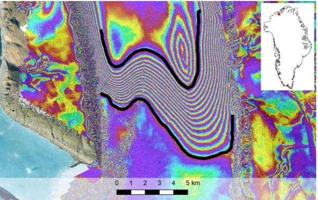
interval and high flow speed (up to 3 m/day). Figure3 shows an interferogram of the grounding 155
zone of Ryder Glacier in north Greenland derived from 6-day repeat pass SAR data of Sentinel-1A 156
and 1B acquired at 6, 12 and 18 January 2017. The grounding zone can be recognized as a distinct 157
band of fringes in the interferogram caused by tidal deformation. 158
Figure 3.Geocoded double difference interferogram of the grounding zone of Ryder Glacier derived from repeat pass SAR data of Sentinel-1A and 1B acquired at 6, 12 and 18 January 2017 (background: Google Earth). Thick black lines indicate the lower and upper boundary of the tidal flexure zone. Inset shows location of Ryder Glacier in North Greenland.
3.4. Surface Elevation Change 159
The surface elevation change (SEC) is based on satellite radar altimeter observations from 160
1992-2017. The time series of observations is averaged as 5-year running mean estimates, to 161
reflect climate variability and not weather. The SEC estimation uses a combination of cross-over-, 162
repeat-track- and least-squares-methods to estimate the temporal evolution of surface elevation at a 163
common 5 km uniformed grid for the entire GrIS, for more detail into the specific methods we refer the 164
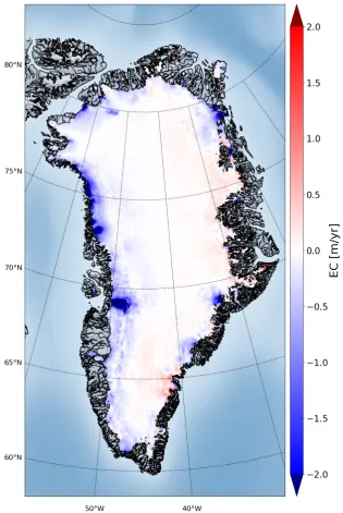
reader to the method review in [5] and mission specific papers [2,4,22–25]. Figure4shows the 5-year 165
running mean estimate, for the period 2012 to 2016 in which the observed negative elevation change 166
on the GrIS is clearly observed, particularly at the margins and in agreement with the literature 167
[26,27]. The observed SEC is compared with RCM and ISM results (see section 3.6 and 3.7) to infer 168
Figure 4. (Upper panel) Mean surface elevation change over the GrIS for 2016 and 2017 of the GrIS from radar altimetry
3.5. Gravimetric Mass Balance from GRACE 170
The ESA GrIS CCI project provides estimates of ice mass balance derived from the joint NASA / 171
DLR GRACE (Gravity Recovery & Climate Experiment) mission [28]. The GRACE mission consisted 172
of two identical spacecrafts flying about 220 km apart in a polar orbit originally at 480 km above 173
the Earth mapping the Earth’s gravity field each month. Mapping directly the Earth’s gravity field 174
GRACE is the only remote sensing data set, which directly measures mass change, and thereby 175
observes the ice mass balance (or equivalent sea-level rise). 176
The monthly solutions (level 2 product) are provided as spherical harmonic coefficients (e.g. up 177
to degree lmax=96) by different processing centers such as CSR, GFZ, JPL and more recently also by 178
TU Graz (ITSG-Grace2016) [29]. As a part of the ESA GrIS CCI project, Gravimetric Mass Balance 179
(GMB) products are generated using both both ITSG-Grace2016 (2002-2017) and the new CSR RL06 180
and TU Dresden (TUDR) using different approaches. The GMB products comprise mass change time 182
series for eight drainage basins [31] and the entire GrIS as well as gridded mass balance estimates 183
over running 5-year periods. 184
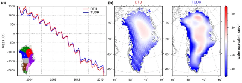
Figure 5. GMB products provided by the ESA GrIS CCI project. a) Mass change time series for the entire GrIS generated by DTU (red) and TUDR (blue). b) Ice mass trends for 2007-2011 provided by DTU (left) and TUDR (right). All products based on monthly solutions from the ITSG-Grace2016 series.
DTU applies an inversion technique to derive monthly mass changes. Gravity observations at 185
satellite altitude are used to solve for point masses on an icosahedron grid, where each point mass 186
represents an area with a radius of∼ 20 km. The ice mass changes over the whole GrIS are derived 187
including the peripheral glaciers, which cannot discriminate in the∼ 300 km resolution of GRACE. 188
A detailed description of the approach is given in [30]. TUDR estimates monthly mass changes by 189
applying a regional integration approach per grid cell of a 50×50 km2 grid. For each grid cell a 190
tailored sensitivity kernel was designed, which minimizes the sum of GRACE errors, derived from 191
empirical error variance-covariance information, and signal leakage [32]. Mass change time series per 192
drainage basin are derived by simply integrating the corresponding point masses or grid cells. Figure 193
5shows two types of GMB products derived by the different approaches. 194
Published studies (e.g.[33]) use surface mass balance estimates derived from the RACMO 195
regional climate model to assess the relative importance of surface and dynamic processes to ice sheet 196
mass change. The relatively high resolution and apparently reasonable performance of such models 197
in calculating SMB means that basin scale ice dynamics can be resolved for the GrIS. In this study we 198
compare the results from the HIRHAM5 RCM with published results using the RACMO RCM [1,34]. 199
Although the two RCMs compared here are remarkably similar (see section 4.3), this breakdown also 200
allows us to assess processes that give rise to divergence between RCMs and the implications of these 201
processes for assessing uncertainties in ice sheet mass balance. 202
3.6. Regional Climate Model HIRHAM5 203
The Regional Climate Model HIRHAM5 as described in [10,35] is used in this study as climate 204
forcing. HIRHAM5 is run at 0.05 degrees (5.5km) resolution on a rotated polar grid, and forced 205
on the lateral boundaries with temperature, relative humidity, wind components and pressure at all 206
31 levels in the atmosphere every 6 hours from the ERA-Interim climate reanalysis dataset [36]. The 207
lower boundary sea surface temperatures and sea ice applied daily are also derived from ERA-Interim 208
data. The climate model was developed at the Danish Meteorological Institute with physical schemes 209
modified from ECHAM5 physics [37] to be suitable for application in polar regions [38,39]. The 210
dynamical equations are derived from the HIRLAM7 numerical weather prediction model [40]. The 211
atmospheric radiative and turbulent fluxes drive a surface energy balance model to calculate melt 212
SMB model includes a multi-layer firn model that accounts for retention and refreezing of meltwater 214
within the snowpack [10,39]. The effects of retention and refreezing are important to account for in 215
calculating surface elevation change as well as having implications for total mass balance. Melt, that 216
can be detected for example by passive microwave sensors [41] does not necessarily mean runoff and 217
mass loss. Modelled SMB combined with GMB allows the partitioning of mass loss from Greenland 218
into atmospherically driven melt and runoff and dynamically influenced calving and basal melt [12, 219
34,42,43]. 220
In this study we also use the SMB calculated in HIRHAM5, together with surface temperatures, 221
to force the parallel ice sheet model (PISM). ISMs are used to derive rates of dynamic mass change 222
and are typically forced with a simplified surface forcing based on temperature and precipitation or, 223
as in this study with a physically based SMB model using a surface energy budget method. 224
3.7. Ice Sheet Modelling with PISM 225
Given the vast amount of feedback mechanisms and interactions involving ice sheets in the 226
climate system, ice sheet modelling and estimating future rates of ice loss is a major challenge [44,45] 227
and has been identified as a major source of uncertainty in sea level rise projections by IPCC authors 228
in the fifth assessment report [8]. Ice sheet models are available at a range of different degrees 229
of complexity, from basic zero order models to hybrid models and second order models to full 230
Stokes models [46]. Each model type has different limitations and strong points and is suitable for 231
different types of simulations spanning a variety of temporal and spatial scales. Regardless of model 232
complexity however, proper boundary and initial conditions are necessary, requiring observational 233
data to be available. Also, in order to validate the models and constrain model parameters, 234
observational data sets are essential. Here, we use SEC data to evaluate simulations of the ice sheet 235
with the Parallel Ice Sheet Model (PISM). 236
PISM is an open-source thermodynamically coupled, polythermal hybrid stress balance ice sheet model [47,48], where the hybrid scheme combines the Shallow Ice Approximation (SIA) [49] and the Shallow Shelf Approximation [50]. The effective viscosity of glacier ice,η, is given by
2η= 1 EA
τe2+ε2
1−2nn
(1)
Eis the flow enhancement factor,τeis the effective stress,Ais the enthalpy-dependent rate factor and
237
εis a small constant regularizing the flow law at low effective stresses, thereby avoiding problems 238
with infinite viscosity at zero deviatoric stress. For the simulations presented here, E = 1.5 and 239
n = 3.0 for both the SIA and the SSA case. Calving is accounted for using a mask reflecting the 240
initial ice geometry but with no further ice dynamical feedback implemented int he model. In order 241
to examine the effects of sliding on the ice flow, different values for the fill value for yield stress of the 242
basal till have been tested, from a value of 2.0·105Pa to 1.25·105Pa, the former being a very strong 243
value, that ensures little or no sliding to amplify the flow [51]. All other model parameters related to 244
sliding are kept constant. 245
The ice sheet model is run over Greenland at 2km grid resolution, with initial bedrock and ice surface 246
topography from [52] and is driven by monthly fields of surface mass balance and 2m temperatures 247
from the regional climate model HIRHAM5 (Sec.3.6) for the period 1980-2017. Prior to the 1980-2017 248
simulation, we made a spinup simulation consisting of a glacial cycle run following the SeaRISE 249
experiments [53] at 10km grid resolution followed by runs at progressively higher model resolution 250
(10km-5km-2km) driven by a constant annual cycle based on multi-year monthly means of the first 251
15 years of the HIRHAM5 1980-2017 time slice in order to bring the ice sheet close to equilibrium with 252
4. Results and Discussion 254
4.1. Surface elevation change in models and observations 255
The relatively short period of observations, compared with the long timescales of ice sheet 256
dynamics makes for challenging evaluation of ice sheet surface elevation change due to ice dynamics. 257
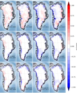
In Figure65 year means of observed SEC are compared with the modelled SEC from the HIRHAM 258
SMB output and the PISM modelled change. In this way the relative contributions of surface and 259
dynamical processes to changes in SEC are decomposed. 260
Figure 6.(Upper panel) Surface elevation of the GrIS from radar altimetry. (Middle panel) Change in surface mass balance in respect to the reference period (1982-1992). (Lower panel) Change in volume as modelled by PISM when forcing PISM with HIRHAM5 surface mass balance and temperature.
Comparison between the SEC observed from radar altimetry (upper panel) with the modelled 261
SMB (middle panel) and modelled SEC from the ISM (lower panel) suggests that surface mass 262
processes of precipitation and melt dominate the observed SEC. This supports analysis by [14] who 263
also found SMB processes dominate the recent ice sheet mass budget. Around the margins of the 264
ice sheet the modelled SMB from the RCM and SEC observations show a similar pattern of elevation 265
change both in sign and in spatial extent. However, it is also noteworthy that the majority of the 266
ice sheet interior shows a small surface increase in all four periods from observations, this is not 267
observed surface elevation increase in this region may also result from ice sheet dynamic processes 269
as suggested by [54] though the ice sheet model also does not capture this process. 270
There are some regions of the GrIS, mainly around basins where there are fast flowing outlet 271
glaciers such as Jakobshavn glacier, that show a surface lowering much greater than derived from the 272
SMB modelling. The PISM model results also show the strong influence of the surface mass balance 273
forcing from HIRHAM though in some regions there is a discernible ice dynamic influence such as 274
in the Jakobshavn basin as well as drainage basins feeding into the fast moving outlet glaciers of 275
south east Greenland. However, the ISM in fact under-predicts this SEC and in some cases even 276
has the wrong sign. This is likely to be at least in part a result of the model resolution inadequately 277
capturing basal topography though may also reflect process parameter uncertainty that gives lower 278
ice sheet velocities than observed in some locations as discussed in the following section. The lack 279
of a dynamic calving parameterisation, a long-standing problem in ice sheet modelling [19], may 280
also contribute to this underestimate in SEC as the model underestimates the increase in ice velocity 281
gradients that lead to dynamic thinning [55] as calving rates increase. 282
4.2. Modelled and Observed Ice Velocities 283
In Figure7the mean modelled ice velocities for the winter 2014-2015 (Oct-Mar) are compared to 284
the corresponding observed ice velocity. Figure7b) shows the results for the low sliding case, while 285
Figure7e) shows the sliding case. In both cases, overall structure of the flow field looks reasonable, 286
even though the modelled velocities are too low. Ice streams are mostly properly located, even though 287
the North Eastern Greenland Ice Stream (NEGIS) is poorly represented. This is however, a consistent 288
feature of ISMs since NEGIS dynamics are believed to be heavily influenced by geothermal heat 289
anomalies [56–58] an effect that is currently not accounted for in most model setups. Here, PISM’s ice 290
streams are generated by bedrock topography and a combination of sliding over the base and shear 291
deformation of a thin till and ice layer at the base [47]. When sliding is included, see Figure. 7e), 292
the overall ice velocity increases and the individual ice streams become more focused. Figure 7d) 293
shows the difference in the modelled velocities. From the difference plot it is evident that the overall 294
velocity of the ice changes very little in the two cases, but the velocity in the ice streams increases 295
significantly and focuses the flow. Using the IV data to tune the sliding enhancement factor provides 296
a better correspondence with the observed ice velocities. 297
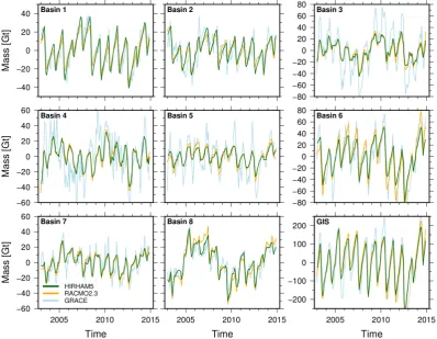
4.3. Partitioning the ice sheet budget 298
To compare surface mass changes modelled by HIRHAM5 and RACMO2.3 [59] with those 299
observed by GRACE, cumulative SMB anomalies are calculated from the monthly SMB values of 300
both models. Long-term signal components are removed by calculating residuals w.r.t. a linear 301
and quadratic model. In this way, the impact of differing reference periods used for deriving the 302
cumulative SMB anomalies and of ice-dynamical mass changes included in the GMB products are 303
largely removed. Figure 8compares residual mass changes for eight drainage basins and the whole 304
GrIS. 305
Overall there is good agreement between models for the ice sheet as a whole with some 306
interesting regional variations. The higher amplitude positive mass balance from GRACE in basins 3, 307
4 and 5 also coincide with regions showing the highest precipitation inputs in Greenland - suggesting 308
that the precipitation over the ice sheet remains a significant source of uncertainty in both models 309
and in terms of decomposing the GRACE land and ice signals. The low SEC calculated from the SMB 310
model compared with the observed surface elevation change in the high interior of the ice sheet also 311
indicates that modelled precipitation from RCMs may be too low over much of the interior. 312
There is relatively little observational data for accumulation rates across Greenland, analysis 313
of field data collected along the Q-transect (the Qassimiut ice lobe), one of the few consistent time 314
series of observations, by [60] demonstrates that in basin 5, both RACMO and HIRHAM5 regional 315
climate models overestimate precipitation over the ice sheet, particularly close to the margin. This 316
has a consequent impact on the modelled melt rate which is therefore lower than observed due to 317
the albedo feedback of bare ice exposure being delayed during the melt season. The underestimate of 318
mass loss in the RCMs compared to the GMB may thus also be partly explained by this underestimate 319
in basin 5. Some of the highest melt rates and highest snowfall rates have been recorded by automatic 320
weather stations on the ice sheet in Greenland in basin 5, regional climate models have struggled 321
to reproduce these observations [60], demonstrating the value in supplementing satellite based 322
observations and models with field measurement campaigns. Overestimating precipitation in high 323
relief topography at the coast in turn likely leads to an underestimate of precipitation in the interior 324
of the ice sheet. 325
The high amplitude mass loss in the GRACE signal, compared to the RCM data that is also 326
especially apparent in basins 3,4 and 5 also suggests the importance of dynamical and ocean driven 327
processes in enhancing mass loss in these regions. Basin 4 in particular has a large number of actively 328
calving glaciers and the large mass loss recorded by the GMB from GRACE but not in the RCMs from 329
2005 to 2008 coincides with a period of retreat and active calving discussed further below. 330
Interestingly, in basins 1 and 2, where calving and ice dynamics are not as large contributors to 331
mass loss as in other regions, modelled SMB and GMB data products match rather well. However, 332
there are some significant differences between the two RCMs in some years in these regions as 333
well as in region 8. We hypothesise that some of the variation is due to the albedo effect and 334
differing albedo parameterisations as well as perhaps different precipitation rates in the two models 335
in these locations. Northern Greenland has low precipitation rates and once darker glacier ice is 336
exposed after fresh snow with a higher albedo melts away, large amounts of ice can be lost. A 337
small increase in precipitation in one model compared to the other, or conversely a slightly different 338
albedo parameterisation that increases melt in one model compared to the other, can thus have a 339
large impact in these two basins. This analysis shows the value of detailed observations of mass 340
change in interpreting and improving process understanding in Greenland and points to areas where 341
Figure 8.Inter-comparison of mass changes from GRACE (GrIS CCI GMB product) and two regional climate models (HIRHAM5 and RACMO2.3) for different drainage basins (cf. inset in Figure 5) and the entire GrIS. Mass changes are given w.r.t. a linear and quadratic model.
4.4. Modelling mass change from Radar Altimetry 343
The Ku-radar band utilized by ESA radar altimeter satellites, will penetrate the upper snow 344
surface of ice sheets and give a return formed by volume scattering of the penetrated snow. If this 345
snow pack suddenly incorporates ice lenses this might act as the stronger reflector and dominate the 346
return echo. As highlighted by the 2012 extreme melt event on the Greenland [61] radar altimetry is 347
hampered by mapping changes in the reflective horizon of the ice sheet [62], and needs to be corrected 348
for in the interpretation of mass balance. On the other hand, the ability to penetrate the surface snow 349
can be utilized when mapping mass change [63], assuming surface elevation variability from light 350
and heavy snowfall events is filtered-out by the radar penetrating a finite volume in terms of mass. 351
Traditionally, laser altimetry mapping surface elevation changes have been converted into mass 352
by applying a firn model [7,64]. Here, we omit the correction terms and use the knowledge gained 353
about mass changes in the ICESat era by [7], to estimate a scaling factor between radar and lidar mass 354
balance estimates at 100 km resolution. The low spatial resolution limits the needs for a physical 355
model for elevation to mass change conversion, but favour a general empirical relationship as found 356
by scaling to ICESat data. Figure9show the 25 year mass balance record for the Greenland ice sheet 357
from assigning an appropriate density to the elevation change mapped by radar altimetry and our 358
best estimate of the mass balance of the Greenland ice sheet applying the scaling to ICESat data. The 359
GRACE record is also shown in the figure as reference. It is important to note that the method cannot 360
map fast changes in the mass change as observed in recent years, these also are mapped into the error 361
bounds. This is expected as wider footprint of the radar altimeter has challenges in capturing the 362
high-slop and fast changing outlet-glaciers of the Greenland ice sheet. From the record the ice sheet is 363
Figure 9. GrIS volume change estimates, including the raw (blue) mass change from radar altimetry (RA). The black line indicates the average radar altimetry rate during the ICESat era, the red line indicates the average rate measured by ICESat. The calibrated radar altimetry mass change rate is shown with uncertainties in cyan. For reference the GRACE mass change rate is shown in green.
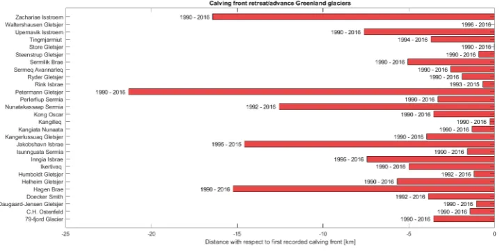
4.5. Calving glacier retreat and ice sheet mass budget 365
Understanding calving processes is important as increased calving rates significantly contribute 366
to an increase in mass loss from the Greenland ice sheet, with [1,14,34] suggesting around one third 367
of ice lost from the GrIS was the result of iceberg calving and related processes. Out of the 28 glaciers 368
monitored by the CCI project, all except two underwent significant retreat during the period 1990 to 369
2016 (Figure10). 370
Figure 10. Total calving front retreat for each of 28 outlet glaciers between the 1990s and 2016 (top). The annually averaged rate of position change over the period (bottom).
As calving rates and calving front location (CFL) are controlled by multiple processes ([19]), the 371
total location change and therefore rate are very sensitive to the start and end dates chosen. As Figure 372
11shows, CFL is often at a stable position for a decade or longer, before a calving retreat that leads to 373
a rapid change in position before establishing a new stable location. At Petermann glacier, a floating 374
ice shelf rather than a tidewater glacier, the CFL gradually moves forward before a single calving 375
event shortened the ice shelf dramatically, after which the CFL again started to move forward again. 376
The episodic nature of changes in CFL emphasises the need for long-term monitoring to understand 377
the behaviour of calving fronts. 378
Figure 11. (left) Calving front location between 1995 and 2015. (right) Average distance between a reference grounding line of 1995 and the calving front.
The time series in the CFL dataset are at least 20 years and in some cases almost 30 years 379
suggesting that the consistent retreat of glaciers observed around Greenland is the result of 380
widespread climate change in the region. 381
4.6. Grounding Line Stability and Ice Shelf Fracture Processes 382
Most of the calving outlet glaciers in Greenland are tidewater type, that is with usually only 383
reminiscent of the large Antarctic ice shelves do exist, although largely only in confined fjord settings 385
unlike those found around the Antarctic continent. Plotting the grounding line locations on these 386
floating ice shelves proved technically challenging but the stability of these locations as for example 387
shown by [16] suggests that these glaciers are mostly stable in position at least at present day climate. 388
Glaciers with floating ice shelves such as Petermann, 79 fjord and Zachariae Isstrøm as well as Hagen 389
glacier are significant because each of these glacier draw down relatively large proportions of the 390
ice sheet and so collapse could potentially lead to rapid and unstable sea level rise. For this reason, 391
we present a case study at Petermann glacier, where multiple datasets including the ice velocity, 392
grounding line and calving front location were combined with modelled surface runoff and an ice 393
fracture model to give an insight into calving processes and to examine how stable the Petermann 394
glacier ice shelf is at the present day extent (Figure11). 395
Ice velocity data is used to derive strain rates that in turn are used to calculate crevasse 396
penetration depths [65]. These have been implemented as a parameterisation in ISMs to determine 397
calving front location and the associated dynamic feedbacks (e.g.[55]). The CCI IV data products are 398
therefore an ideal opportunity to derive strain rates and constrain estimates of calving activity based 399
on these (Figure12B). 400
Using Glen’s flow law [66] the principle stresses are calculated from the strain rates derived 401
from IV data. Linear elastic fracture mechanics allows for the calculation of the penetration depth 402
a crevasse will reach considering the calculated stress [65,67]. Besides the stress acting on the ice, 403
the spacing between crevasses and the presence of water in crevasses are strong determinants of the 404
depth a crevasse can reach and whether or not calving will occur as shown in Figure:12C,D. The 405
presence of water in crevasses enhances crevasse penetration and can lead to fractures propagating 406
through the entire thickness of the ice sheet [19,65]. 407
At Petermann glacier in northern Greenland, liquid water in crevasses is present only during the 408
summer months when the run-off is larger than zero (Figure12A). Analysis of the ice velocity dataset 409
shows that velocity increases significantly in summerm, likely due to melt water at the bed of the 410
Petermann glacier reducing basal pressure as also documented at Zachariae Isstrøm [17,68]. Melt and 411
runoff from the RCM HIRHAM5 is compared with the ice velocity and principal strain rate over the 412
lower part of the ice shelf in Figure12A and B. 413
The importance of fracture spacing and water in enhanced fracture penetration at Petermann 414
glacier is demonstrated by Figure12C and D. The sensitivity of the fracture depth to water suggests 415
that under a warming climate with greater meltwater production at the surface, the ice shelf may well 416
be vulnerable to break up as other glaciers in this region have also collapsed, for example the retreat 417
at C.H. Ostenfeldt glacier shown in Figure10and described along with other Greenland glaciers by 418
[69]. Equally, higher velocities, leading to higher strain rates could lead to deeper fractures, though 419
this effect is reduced somewhat if more crevasses open since the crevasse spacing also affects the 420
depth of an individual fracture Figure12D. [35,43] show a significant increase in melt water runoff 421
across Greenland under two different climate change scenarios, indicating that floating ice shelves 422
like Petermann glacier may become vulnerable in future, a conclusion supported by [68]. Extending 423
this analysis at Petermann glacier to other outlet glaciers covered by the CCI GrIS datasets will also 424
give a wider indication of the potential stability of outlet glaciers, but is beyond the scope of the 425
current work. 426
5. Outlook 427
In this review paper we have given an overview of the current mass budget of the Greenland 428
ice sheet based on models and remote sensing observations. We have also examined the relative 429
contributions from surface mass budget processes and ice dynamics, including calving processes 430
and grounding lines. The ESA CCI Greenland Ice Sheet observational datasets have proved to 431
be a powerful tool in understanding and improving estimates of ice sheet mass budget and the 432
contribution to sea level rise as well as pinpointing areas where process understanding needs to be 433
improved. The continuation of the generated datasets and extension both back in time where possible 434
using data from older sensors is planned as part of the CCI+ project due to commence in 2019. The 435
existing data products will be enhanced with an ice mass flux and discharge data set that combines 436
remote sensing and model data to give a continually updated reconciled Greenland ice sheet mass 437
budget as used for example in [12]. The successful launch of GRACE- Follow On (GRACE-FO) 438
and continuing developments of the next generation of RCMs and climate reanalysis capable 439
of calculating more accurate SMB, for example the non-hydrostatic model HARMONIE-AROME 440
already used for very high resolution (2.5km) SMB calculations in Greenland [70,71] will also help 441
to reduce process uncertainty. 442
6. Conclusions 443
The Greenland ice sheet has now been observed by satellite and documented in detail for 444
almost three decades. The wealth of detailed information processed and made freely by the ESA 445
climate change initiative has contributed to and will continue to contribute to significant advances in 446
understanding the Greenland ice sheet. 447
Over the period 2002–2015 we find a gravimetric mass balance derived from GRACE for 448
Greenland including the peripheral glaciers and ice caps of 265 +/- 25 GT/year [72]. After the 449
significant acceleration in mass loss rate in the GRACE era up to the record mass loss in the summer 450
of 2012, Greenland has since seen a slight decrease in short-term mass loss trend. 451
Combining data with models is a powerful way to enhance process understanding. 452
Decomposing GMB into basins and comparing with RCM derived SMB suggests models tend to 453
overestimate precipitation over the ice sheet in some key basins and may also underestimate melt 454
rates. At the same time, differences between RCM derived SMB suggests that parameterisations 455
within the models can lead to significant regional biases in mass budget estimates. 456
Surface elevation has reduced across almost all of the ice sheet with a small increase in elevation 457
in the central highest altitude parts of the ice sheet. While RCMs mostly agree with the broad trends 458
in SEC, the inability of RCMs to reproduce the small increase in SEC in the interior and particularly 459
in eastern Greenland suggests that precipitation is underestimated by RCMs and/or that ice dynamic 460
Analysis of model simulations from both regional climate models and ice sheet models 462
demonstrate that while SMB is driving most of the elevation change, some basins demonstrate 463
significant dynamic drawdown related to ice discharge through fast flowing outlet glaciers. However, 464
the inability of the ISM to replicate this entirely suggests that running high resolution models 465
and developing and implementing dynamic feedbacks related to calving retreat are crucial future 466
directions for ice sheet modelling. 467
The active retreat followed by stabilisation of a number of calving outlets is well documented 468
[14] and correlates with the dynamically derived SEC and with areas of relatively high velocity in the 469
ice velocity dataset. 470
Analysis of grounding lines suggests that the few remaining ice shelves are currently relatively 471
stable while analysis of the strain distribution across the ice shelf points to the importance of surface 472
melt water in enhancing fracture propagation. Increases in melt in the future may therefore lead to 473
increased instability and likely collapse of the remaining ice shelves around Greenland. 474
Supplementary Materials:Data Availability 475
All ESA CCI data products are available from the CCI data portal. 476
http://esa-icesheets-greenland-cci.org/ 477
HIRHAM5 regional climate model simulation data can be downloaded from the link given here: 478
http://polarportal.dk/groenland/links/ 479
Acknowledgments: ESA CCI Greenland was funded via ESA-ESRIN contract number 4000104815/11/I-NB. 480
HIRHAM5 regional climate model simulations were carried out by Ruth Mottram with funding from 481
the European Research Council under the European Community’s Seventh Framework Programme (FP7/ 482
2007-2013)/ERC grant agreement 610055 as part of the ice2ice project. 483
Author Contributions:RM and SBS conceived and designed the outline for the paper. RM ran the HIRHAM5 484
regional climate model and analysed the output. SBS and LSS derived altimetry results. AG and VRB estimated 485
the Mass Balance from GRACE with input from MH. SHS performed ice sheet model study and comparisons 486
between ice sheet model output and observations. RF lead the ESA CCI project for the Greenland Ice Sheet. TN 487
and JW derived the ice velocity results. JR and RM developed and ran the calving and ice fracture model. All 488
authors contributed to writing the paper and analyzing the results. 489
Conflicts of Interest:The authors declare no conflict of interest. 490
References 491
1. van den Broeke, M.R.; Enderlin, E.M.; Howat, I.M.; Kuipers Munneke, P.; Noël, B.P.Y.; van de Berg, W.J.; 492
van Meijgaard, E.; Wouters, B. On the recent contribution of the Greenland ice sheet to sea level change. 493
The Cryosphere2016,10, 1933–1946. 494
2. Sørensen, L.S.; Simonsen, S.B.; Meister, R.; Forsberg, R.; Levinsen, J.F.; Flament, T. Envisat-derived 495
elevation changes of the Greenland ice sheet, and a comparison with ICESat results in the accumulation 496
area. Remote Sensing of Environment2015,160, 56–62. 497
3. Nagler, T.; Rott, H.; Hetzenecker, M.; Wuite, J.; Potin, P. The Sentinel-1 Mission: New Opportunities for 498
Ice Sheet Observations. Remote Sensing2015,7, 9371–9389. 499
4. Simonsen, S.B.; Sørensen, L.S. Implications of changing scattering properties on Greenland ice sheet 500
volume change from Cryosat-2 altimetry.Remote Sensing of Environment2017,190, 207–216. 501
5. Sandberg Sørensen, L.; Simonsen, S.B.; Forsberg, R.; Khvorostovsky, K.; Meister, R.; Engdahl, M.E. 25 502
years of elevation changes of the Greenland Ice Sheet from ERS, Envisat, and CryoSat-2 radar altimetry. 503
Earth and Planetary Science Letters2018,495, 234–241. 504
6. Simonsen, S.B.; Stenseng, L.; A ¯dalgeirsdóttir, G.; Fausto, R.S.; Hvidberg, C.S.; Lucas-Picher, P. Assessing 505
a multilayered dynamic firn-compaction model for Greenland with ASIRAS radar measurements.Journal 506
of Glaciology2013,59, 545–558. 507
7. Sørensen, L.S.; Simonsen, S.B.; Nielsen, K.; Lucas-Picher, P.; Spada, G.; Adalgeirsdottir, G.; Forsberg, R.; 508
Hvidberg, C.S. Mass balance of the Greenland ice sheet (2003–2008) from ICESat data – the impact of 509
interpolation, sampling and firn density.The Cryosphere2011,5, 173–186. 510
8. Vaughan, D.G.; Comiso, J.C.; Allison, I.; Carrasco, J.; Kaser, G.; Kwok, R.; Mote, P.; Murray, T.; Paul, F.; 511
9. Cappelen, J. Greenland-DMI historical climate data collection 1784-2017. Danish Meteorological Institue 513
Report 18-042017. 514
10. Langen, P.L.; Fausto, R.S.; Vandecrux, B.; Mottram, R.H.; Box, J.E. Liquid Water Flow and Retention on the 515
Greenland Ice Sheet in the Regional Climate Model HIRHAM5: Local and Large-Scale Impacts. Frontiers 516
in Earth Science2017,4. 517
11. Rignot, E.; Fenty, I.; Xu, Y.; Cai, C.; Kemp, C. Undercutting of marine-terminating 518
glaciers in West Greenland. Geophysical Research Letters, 42, 5909–5917, 519
[https://agupubs.onlinelibrary.wiley.com/doi/pdf/10.1002/2015GL064236]. 520
12. Shepherd, A.; Ivins, E.R.; A, G.; Barletta, V.R.; Bentley, M.J.; Bettadpur, S.; Briggs, K.H.; Bromwich, D.H.; 521
Forsberg, R.; Galin, N.; Horwath, M.; Jacobs, S.; Joughin, I.; King, M.A.; Lenaerts, J.T.M.; Li, J.; Ligtenberg, 522
S.R.M.; Luckman, A.; Luthcke, S.B.; McMillan, M.; Meister, R.; Milne, G.; Mouginot, J.; Muir, A.; Nicolas, 523
J.P.; Paden, J.; Payne, A.J.; Pritchard, H.; Rignot, E.; Rott, H.; Sorensen, L.S.; Scambos, T.A.; Scheuchl, 524
B.; Schrama, E.J.O.; Smith, B.; Sundal, A.V.; van Angelen, J.H.; van de Berg, W.J.; van den Broeke, M.R.; 525
Vaughan, D.G.; Velicogna, I.; Wahr, J.; Whitehouse, P.L.; Wingham, D.J.; Yi, D.; Young, D.; Zwally, H.J. A 526
Reconciled Estimate of Ice-Sheet Mass Balance. Science2012,338, 1183–1189. 527
13. WCRP Global Sea Level Budget Group. Global Sea Level Budget 1993–Present. Earth System 528
Science Data Discussions2018, pp. 1–88. 529
14. Enderlin, E.M.; Howat, I.M.; Jeong, S.; Noh, M.J.; Angelen, J.H.; Broeke, M.R. An 530
improved mass budget for the Greenland ice sheet. Geophysical Research Letters, 41, 866–872, 531
[https://agupubs.onlinelibrary.wiley.com/doi/pdf/10.1002/2013GL059010]. 532
15. Joughin, I.; Fahnestock, M.; Kwok, R.; Gogineni, P.; Allen, C. Ice flow of Humboldt, Petermann and Ryder 533
Gletscher, northern Greenland.Journal of Glaciology1999,45, 231–241. 534
16. Hogg, A.E.; Shepherd, A.; Gourmelen, N.; Engdahl, M. Grounding line migration from 1992 to 2011 on 535
Petermann Glacier, North-West Greenland. Journal of Glaciology2016,62, 1104–1114. 536
17. Rathmann, N.M.; Hvidberg, C.S.; Solgaard, A.M.; Grinsted, A.; Gudmundsson, G.H.; Langen, 537
P.L.; Nielsen, K.P.; Kusk, A. Highly temporally resolved response to seasonal surface melt of the 538
Zachariae and 79N outlet glaciers in northeast Greenland. Geophysical Research Letters, 44, 9805–9814, 539
[https://agupubs.onlinelibrary.wiley.com/doi/pdf/10.1002/2017GL074368]. 540
18. Boncori, J.P.M.; Andersen, M.L.; Dall, J.; Kusk, A.; Kamstra, M.; Andersen, S.B.; Bechor, N.; Bevan, S.; 541
Bignami, C.; Gourmelen, N.; Joughin, I.; Jung, H.S.; Luckman, A.; Mouginot, J.; Neelmeijer, J.; Rignot, E.; 542
Scharrer, K.; Nagler, T.; Scheuchl, B.; Strozzi, T. Intercomparison and Validation of SAR-Based Ice Velocity 543
Measurement Techniques within the Greenland Ice Sheet CCI Project. Remote Sensing2018,10, 929. 544
19. Benn, D.I.; Warren, C.R.; Mottram, R.H. Calving processes and the dynamics of calving glaciers. 545
Earth-Science Reviews2007,82, 143–179. 546
20. Rignot, E.; Velicogna, I.; van den Broeke, M.R.; Monaghan, A.; Lenaerts, J.T. Acceleration of the 547
contribution of the Greenland and Antarctic ice sheets to sea level rise. Geophysical Research Letters2011, 548
38. 549
21. Rignot, E.; Mouginot, J.; Scheuchl, B. Antarctic grounding line mapping from differential satellite radar 550
interferometry: GROUNDING LINE OF ANTARCTICA.Geophysical Research Letters2011,38, n/a–n/a. 551
22. Davis, C.; Ferguson, A. Elevation change of the Antarctic ice sheet, 1995-2000, from ERS-2 satellite radar 552
altimetry. IEEE Transactions on Geoscience and Remote Sensing2004,42, 2437–2445. 553
23. Johannessen, O.M. Recent Ice-Sheet Growth in the Interior of Greenland. Science2005,310, 1013–1016. 554
24. Kirill S. Khvorostovsky. Merging and Analysis of Elevation Time Series Over Greenland Ice Sheet From 555
Satellite Radar Altimetry. IEEE Transactions on Geoscience and Remote Sensing2012,50, 23–36. 556
25. Levinsen, J.; Khvorostovsky, K.; Ticconi, F.; Shepherd, A.; Forsberg, R.; Sørensen, L.; Muir, A.; Pie, N.; 557
Felikson, D.; Flament, T.; Hurkmans, R.; Moholdt, G.; Gunter, B.; Lindenbergh, R.; Kleinherenbrink, 558
M. ESA ice sheet CCI: derivation of the optimal method for surface elevation change detection of the 559
Greenland ice sheet – round robin results.International Journal of Remote Sensing2015,36, 551–573. 560
26. Velicogna, I.; Wahr, J. Acceleration of Greenland ice mass loss in spring 2004. Nature2006,443, 329–331. 561
27. Svendsen, P.; Andersen, O.; Nielsen, A. Acceleration of the Greenland ice sheet mass loss as observed by 562
GRACE: Confidence and sensitivity.Earth and Planetary Science Letters2013,364, 24–29. 563
28. Tapley, B.; Bettadpur, S.; Watkins, M.; Reigber, C. The gravity recovery and climate experiment: Mission 564
29. Mayer-Gürr, T.; Behzadpour, S.; Ellmer, M.; Kvas, A.; Klinger, B.; Zehentner, N. ITSG-Grace2016 – 566
Monthly and Daily Gravity Field Solutions from GRACE.GFZ Data Services2016. 567
30. Barletta, V.R.; Sørensen, L.S.; Forsberg, R. Scatter of mass changes estimates at basin scale for Greenland 568
and Antarctica. The Cryosphere2013,7, 1411–1432. 569
31. Zwally, H.; Giovinetto, M.; Beckley, M.; Saba, J.Antarctic and Greenland Drainage Systems; 2012. 570
32. Groh, A.; Horwath, M. The method of tailored sensitivity kernels for GRACE mass change estimates. 571
Geophysical Research Abstracts2016,18, EGU2016–12065. 572
33. Sasgen, I.; van den Broeke, M.; Bamber, J.; Rignot, E.; Sørensen, L.; Wouters, B.; Martinec, Z.; Velicogna, I.; 573
Simonsen, S. Timing and origin of recent regional ice-mass loss in Greenland. Earth and Planetary Science 574
Letters2012,333-334, 293–303. 575
34. van den Broeke, M.; Bamber, J.; Ettema, J.; Rignot, E.; Schrama, E.; van de Berg, W.J.; van Meijgaard, E.; 576
Velicogna, I.; Wouters, B. Partitioning Recent Greenland Mass Loss. Science2009,326, 984–986. 577
35. Mottram.; Boberg.; Langen.; Yang.; Rodehacke.; Christensen.; Madsen. Surface Mass balance of the 578
Greenland ice Sheet in the Regional Climate Model HIRHAM5: Present State and Future Prospects. Low 579
temperature science2017,75, 1–11. 580
36. Dee, D.P.; Uppala, S.M.; Simmons, A.; Berrisford, P.; Poli, P.; Kobayashi, S.; Andrae, U.; Balmaseda, M.; 581
Balsamo, G.; Bauer, d.P.; others. The ERA-Interim reanalysis: Configuration and performance of the data 582
assimilation system. Quarterly Journal of the royal meteorological society2011,137, 553–597. 583
37. Roeckner, E.; Oberhuber, J.M.; Bacher, A.; Christoph, M.; Kirchner, I. ENSO variability and atmospheric 584
response in a global coupled atmosphere-ocean GCM.Climate Dynamics1996,12, 737–754. 585
38. Rae, J.G.L.; Aðalgeirsdóttir, G.; Edwards, T.L.; Fettweis, X.; Gregory, J.M.; Hewitt, H.T.; Lowe, J.A.; 586
Lucas-Picher, P.; Mottram, R.H.; Payne, A.J.; Ridley, J.K.; Shannon, S.R.; van de Berg, W.J.; van de Wal, 587
R.S.W.; van den Broeke, M.R. Greenland ice sheet surface mass balance: evaluating simulations and 588
making projections with regional climate models. The Cryosphere2012,6, 1275–1294. 589
39. Langen, P.L.; Mottram, R.H.; Christensen, J.H.; Boberg, F.; Rodehacke, C.B.; Stendel, M.; van As, D.; 590
Ahlstrøm, A.P.; Mortensen, J.; Rysgaard, S.; Petersen, D.; Svendsen, K.H.; Aðalgeirsdóttir, G.; Cappelen, J. 591
Quantifying Energy and Mass Fluxes Controlling Godthåbsfjord Freshwater Input in a 5-km Simulation 592
(1991–2012). Journal of Climate2015,28, 3694–3713. 593
40. Eerola, K. Twenty-one years of verification from the HIRLAM NWP system. Weather and Forecasting2013, 594
28, 270–285. 595
41. Mote, T.L.; Anderson, M.R. Variations in snowpack melt on the Greenland ice sheet based on 596
passive-microwave measurements. Journal of Glaciology1995,41, 51–60. 597
42. Ettema, J.; van den Broeke, M.R.; van Meijgaard, E.; van de Berg, W.J.; Bamber, J.L.; Box, J.E.; Bales, R.C. 598
Higher surface mass balance of the Greenland ice sheet revealed by high-resolution climate modeling. 599
Geophysical Research Letters2009,36. 600
43. Fettweis, X.; Franco, B.; Tedesco, M.; van Angelen, J.H.; Lenaerts, J.T.M.; van den Broeke, M.R.; Gallae, 601
H. Estimating the Greenland ice sheet surface mass balance contribution to future sea level rise using the 602
regional atmospheric climate model MAR.The Cryosphere2013,7, 469–489. 603
44. Vizcaino, M. Ice sheets as interactive components of Earth System Models: progress and challenges. 604
WIRES Climate Change2014,5, 557–568. 605
45. Goelzer, H.; Robinson, A.; Seroussi, H.; van de Wal, R.S. Recent Progress in Greenland Ice Sheet 606
Modelling. Current Climate Change Reports2017,3, 291–302. 607
46. Kirchner, N.; Hutter, K.; Jakobsson, M.; Gyllencreutz, R. Capabilities and limitations of numerical ice sheet 608
models; a discussion for Earth-scientists and modelers.Quaternary Science Reviews2011,30, 3691–3704. 609
47. Bueler, E.; Brown, J. The shallow shelf approximation as a ’sliding law’ in a thermomechanically coupled 610
ice sheet model. Journal of Geophysical Research2009,114, 1–21. 611
48. Aschwanden, A.; Bueler, E.; Khroulev, C.; Blatter, H. An enthalpy formulation for glaciers and ice sheets. 612
Journal of Glaciology2012,58, 441–457. 613
49. Theoretical Glaciology: Mateial Science of Ice and the Mechanics of Glaciers and Ice Sheets; Number 1 in 614
Mathematical Approaches to Geophysics, Springer, 1983. 615
50. Morland, L. Plane and Radial Ice-Shelf Flow with Prescirpbed Temperature Profile. InDynamics of the 616
West Antarctic Ice Sheet; van der Veen, C.J. and Oelemans, J.., Ed.; D. Reidel Publishing Company, 1987. 617
52. Bamber, J.; Layberry, R.; Gogenini, S. A new ice thickness and bed data set for the Greenland ice sheet1: 619
Measurement, data reduction, and errors.Journal of Geophysical Research2001,106, 33773–33780. 620
53. Nowicki, S.; Bindschadler, R.A.; Abe-Ouchi, A.; Aschwanden, A.; Bueler, E.; Choi, H.; Fastook, J.; 621
Granzow, G.; greve, R.; Gutowski, G.; Herzfeld, U.; Jackson, C.; Johnson, J.; Khroulev, C.; Larour, E.; 622
Levermann, A.; Lipscomb, W.H.; Martin, M.A.; Morlighem, M.; Parizek, B.R.; Pollard, D.; Price, S.F.; Ren, 623
D.; Rignot, E.; Saito, F.; Sato, T.; Seddik, H.; Seoussi, H.; Takahashi, K.; Walker, R.; Wang, W.L. Insight into 624
spatial sensitivities of ice mass response to environmental change from the SeaRISE ice sheet modeling 625
project II: Greenland.Journal of Geophysical Research2013,118, 1025–1044. 626
54. Colgan, W.; Rajaram, H.; Abdalati, W.; McCutchan, C.; Mottram, R.; Moussavi, M.S.; Grigsby, S. Glacier 627
crevasses: Observations, models, and mass balance implications: Glacier Crevasses. Reviews of Geophysics 628
2016,54, 119–161. 629
55. Nick, F.; Van Der Veen, C.; Vieli, A.; Benn, D. A physically based calving model applied to marine outlet 630
glaciers and implications for the glacier dynamics.Journal of Glaciology2010,56, 781–794. 631
56. Fahnestock, M.; Abdalati, W.; Joughin, I.; Brozena, J.; Gogineni, P. High Geothermal Heat Flow, Basal 632
Melt, and the Origin of Rapid Ice Flow in Central Greenland. Science2001,294, 2338–2342. 633
57. Christanson, K.; Peters, L.E.; Alley, R.B.; Anandakrishnan, S.; Jacobel, R.W.; Riverman, K.L.; Muto, A.; 634
Keisling, Benjamin, A. Dilatant till facilitates ice-stream flow in northeast Greenland. Earth and Planetary 635
Science Letters2014,401, 57–69. 636
58. Rogozhina, I.; Petrunin, A.G.; P.M, V.A.; Steinberger, B.; Johnson, J.V.; Kaban, M.K.; Reinhard, C.; Rickers, 637
F.; Thomas, M.; Koulakov, I. Melting at the base of the Greenland ice sheet explained by Iceland hotspot 638
history. Nature Geoscience2016,9, 366–369. 639
59. Noel, B.; van de Berg, W.; van Meijgaard, E.; Kuipers Munneke, P.; van de Wal, R.; van den Broeke, M. 640
Evaluation of the updated regional climate model RACMO2.3: summer snowfall impact on the Greenland 641
Ice Sheet. The Cryosphere2015,9, 1831–1844. 642
60. Hermann, M.; Box, J.E.; Fausto, R.S.; Colgan, W.T.; Langen, P.L.; Mottram, R.; Wuite, J.; Noël, B.; van den 643
Broeke, M.R.; van As, D. Application of PROMICE Q-Transect in Situ Accumulation and Ablation 644
Measurements (2000-2017) to Constrain Mass Balance at the Southern Tip of the Greenland Ice Sheet. 645
Journal of Geophysical Research: Earth Surface2018,123, 1235–1256. 646
61. Nghiem, S.V.; Hall, D.K.; Mote, T.L.; Tedesco, M.; Albert, M.R.; Keegan, K.; Shuman, C.A.; DiGirolamo, 647
N.E.; Neumann, G. The extreme melt across the Greenland ice sheet in 2012: EXTREME MELT ACROSS 648
GREENLAND ICE SHEET.Geophysical Research Letters2012,39. 649
62. Nilsson, J.; Vallelonga, P.; Simonsen, S.B.; Sørensen, L.S.; Forsberg, R.; Dahl-Jensen, D.; Hirabayashi, M.; 650
Goto-Azuma, K.; Hvidberg, C.S.; Kjaer, H.A.; Satow, K. Greenland 2012 melt event effects on CryoSat-2 651
radar altimetry: EFFECT OF GREENLAND MELT ON CRYOSAT-2. Geophysical Research Letters2015, 652
42, 3919–3926. 653
63. McMillan, M.; Leeson, A.; Shepherd, A.; Briggs, K.; Armitage, T.W.K.; Hogg, A.; Kuipers Munneke, P.; 654
van den Broeke, M.; Noël, B.; van de Berg, W.J.; Ligtenberg, S.; Horwath, M.; Groh, A.; Muir, A.; Gilbert, 655
L. A high-resolution record of Greenland mass balance: High-Resolution Greenland Mass Balance. 656
Geophysical Research Letters2016,43, 7002–7010. 657
64. Zwally, H J..; Li, J.; Brenner, A C.; Beckley, M.; Cornejo, Helen G.; DiMarzio, J.; Giovinetto, M B.; 658
Neumann, T.~A..; Robbins, J.; Saba, J L.; Yi, D..; Wang, W.. Greenland ice sheet mass balance: distribution 659
of increased mass loss with climate warming; 2003-07 versus 1992-2002.Journal of Glaciology2011,57. 660
65. Mottram, R.H.; Benn, D.I. Testing crevasse-depth models: a field study at Breidamerkurjokull, Iceland. 661
Journal of Glaciology2009,55, 746–752. 662
66. Glen, J.W. The Creep of Polycrystalline Ice. Proceedings of the Royal Society A: Mathematical, Physical and 663
Engineering Sciences1955,228, 519–538. 664
67. van der Veen, C. Fracture mechanics approach to penetration of surface crevasses on glaciers.Cold Regions 665
Science and Technology1998,27, 31–47. 666
68. Nick, F.; Luckman, A.; Vieli, A.; Van Der Veen, C.; Van As, D.; Van De Wal, R.; Pattyn, F.; Hubbard, 667
A.; Floricioiu, D. The response of Petermann Glacier, Greenland, to large calving events, and its future 668
stability in the context of atmospheric and oceanic warming.Journal of Glaciology2012,58, 229–239. 669
69. Hill, E.A.; Carr, J.R.; Stokes, C.R.; Gudmundsson, G.H. Dynamic changes in outlet glaciers in northern 670
70. Mottram, R.; Nielsen, K.P.; Gleeson, E.; Yang, X. Modelling Glaciers in the HARMONIE-AROME NWP 672
model. Advances in Science and Research2017,14, 323–334. 673
71. Bengtsson, L.; Andrae, U.; Aspelien, T.; Batrak, Y.; Calvo, J.; de Rooy, W.; Gleeson, E.; Hansen-Sass, 674
B.; Homleid, M.; Hortal, M.; Ivarsson, K.I.; Lenderink, G.; Niemelä, S.; Nielsen, K.P.; Onvlee, J.; 675
Rontu, L.; Samuelsson, P.; Muñoz, D.S.; Subias, A.; Tijm, S.; Toll, V.; Yang, X.; Koeltzow, M.O. The 676
HARMONIE–AROME Model Configuration in the ALADIN–HIRLAM NWP System. Monthly Weather 677
Review2017,145, 1919–1935. 678
72. Forsberg, R.; Sørensen, L.; Simonsen, S. Greenland and Antarctica ice sheet mass changes and effects on 679