Hiermeyer, Martin (2009): Four Empirical Essays on the Economics of Height. Dissertation, LMU München: Volkswirtschaftliche Fakultät

Full text

(1)Four Empirical Essays on the Economics of Height. INAUGURAL-DISSERTATION. zur Erlangung des Grades Doctor oeconomiae publicae (Dr. oec. publ.) an der Ludwig-Maximilians-Universität München. 2008. vorgelegt von Martin Hiermeyer. Referent:. Prof. John Komlos, Ph.D.. Korreferent:. Prof. Dr. Ekkehart Schlicht. Promotionsabschlussberatung:. 4. Februar 2009.

(2) Four Empirical Essays on the Economics of Height. INAUGURAL-DISSERTATION Submitted to the Department of Economics in partial fulfillment of the requirements for the degree of Doctor oeconomiae publicae (Dr. oec. publ.) at the Ludwig-Maximilians-University Munich. 2008. Martin Hiermeyer. Thesis Supervisor:. Prof. John Komlos, Ph.D.. Thesis Co-Supervisor. Prof. Dr. Ekkehart Schlicht. Final Committee Consultation:. February 4th, 2009.

(3) To Milenka.

(4) Acknowledgements First and foremost, I would like to thank my supervisor, Professor John Komlos, for his outstanding support and academic guidance. I am deeply indebted to him for taking such an extraordinary amount of time to comment on each of my papers. I cannot imagine better support. I am also very grateful to Professor Ekkehart Schlicht for his feedback and for kindly accepting to be co-supervisor. Furthermore, I would like to thank Professor Joachim Winter for agreeing to complete my thesis committee as third examiner. Special thanks go to my former and current colleagues Ariane Breitfelder, Francesco Cinnirella, Arne Kues, Marco Sunder, Gordon Winder, and Matthias Zehetmayer for valuable comments and for providing me with a very pleasurable work and research environment. I would also like to thank the participants of various research workshops at the University of Munich, in particular Jörg Baten, Roberto Cruccolini, Helmut Küchenhoff, Elmar Nubbemeyer, and Christoph Stoeckle. I am grateful to Detlef Kaltwasser (Statistisches Bundesamt), Rainer Lüdde (Institut für Wehrmedizinalstatistik und Berichtswesen), Steve McClaskie (US Bureau of Labor Statistics), and Heribert Stolzenberg (Robert-Koch-Institute) for helping me to fully understand the data sets used in this dissertation. Parts of this doctoral thesis were written during my research stay at the University of Cambridge. I am particularly indebted to Sheilagh Ogilvie who served as my supervisors there. I also owe gratitude to Christian Grisse, Gisela Jäger, Cherie Lee, and Craig Peacock. Financial support from Deutscher Akademischer Austauschdienst (DAAD), grant no. D/07/41734, is gratefully acknowledged. Last but certainly not least I would like to thank my whole family..

(5) Table of Contents 1.. Introduction. 12. 1.1. The Economics of Height. 13. 1.2. References. 16. The Correlation between Height and Wages, a Conundrum Explored. 18. 2.1. Abstract. 19. 2.2. Introduction. 19. 2.3. Data. 21. 2.4. The relationship between height and wages in the NLSY 97. 31. 2.5. Parental income during adolescence and adult height. 32. 2.6. Channels. 34. 2.7. Conclusion. 38. 2.8. References. 39. 2.9. Appendix. 48. 2.. 3.. The Trade-off between a High and an Equal Biological Standard of Living – Evidence from Germany. 50. 3.1. Abstract. 51. 3.2. Introduction. 51. 3.3. Data. 53. 3.4. Level of the biological standard of living in East and West Germany before. 3.5. and after unification. 56. Regional height convergence in East and West Germany. 68.

(6) 3.6. Inequality in the biological standard of living in East and West Germany before and after unification. 72. 3.7. Regional equality convergence in East and West Germany. 83. 3.8. Conclusion. 84. 3.9. References. 86. 3.10 Appendix. 4.. 93. The Height and BMI values of West Point Cadets after the Civil War. 95. 4.1. Abstract. 96. 4.2. Introduction. 96. 4.3. Data. 97. 4.4. Results. 98. 4.5. Conclusion. 106. 4.6. References. 108. 4.7. Appendix. 113. Height and BMI values of German conscripts in 2000 and 2001. 117. 5.1. Abstract. 118. 5.2. Introduction. 118. 5.3. Data. 119. 5.4. Results. 122. 5.5. Historical comparison. 129. 5.6. Conclusion. 137. 5.7. References. 139. 5.8. Appendix. 143. 5..

(7) Eidesstattliche Versicherung. 146. Curriculum Vitae. 147. List of Tables Table 2.1:. Characteristics of the NLSY sample. Table 2.2:. OLS estimates, dependent variable: log hourly wage of US-born individuals who worked 1,000 hours or more in 2004, age 19-24. Table 2.3:. 31. OLS estimates, dependent variable: adult height of US-born individuals, age 19-24. Table 2.4:. 22. 32. OLS estimates, dependent variable: adult height of white US-born females, age 19-24. 36. Table A2.1:. Survey year and NLSY code for variables used in the paper. 48. Table 3.1:. OLS estimates, dependent variable: adult height of 1930-79 birth cohorts. 59. Table 3.2:. Pre-unification OLS estimates, dependent variable: adult height of 1940-69 birth cohorts. Table 3.3:. Post-unification OLS estimates, dependent variable: adult height of 1980-1983 birth cohorts. Table 3.4:. 64. Separate OLS estimates for West and East Germany, dependent variable: adult height of 1940-69 birth cohorts. Table 3.5:. 63. 67. OLS estimates, dependent variable: difference in average height between the 1946-49 and the 1976-79 birth cohorts. 71.

(8) Table 3.6:. OLS estimates, dependent variable: difference in the coefficient of variation for height between the 1946-49 and the 1976-79 birth cohorts. Table A3.1:. Characteristics of the sample after excluding all observations without height information. Table 4.1:. 83. 93. OLS estimates, dependent variables: height and BMI of West Point cadets (age 16-21) born 1860 to 1884. Table A41:. Characteristics of the combined and new sample. Table 5.1:. OLS estimates, dependent variables: adult height and BMI of German. 99 113. recruits, 2000 and 2001. 122. Table A5.1:. Characteristics of the sample. 143. Table A5.2:. Provinces of the German Empire and today’s states and regions. 144.

(9) List of Figures Figure 2.1:. Scatter diagram between height at age 14 and adult height for white, US-born individuals. Figure 2.2:. Histogram of female (left panel) and male (right panel) height, 14-year old, US-born individuals. Figure 2.3:. 28. Comparison of NLSY 97 and NHANES 1999-2004 growth profiles, US-born individuals only. Figure 2.5:. 27. Histogram of female (left panel) and male (right panel) adult height, US-born individuals only. Figure 2.4:. 25. 29. Average adult height of white US-born females with parents of average height as a function of parental yearly gross household income during adolescence. Figure 2.6:. Average adult height of white US-born females with parents of average height and average income as a function of doctor visits. Figure A2.1: US Census Regions Figure 3.1:. 34. 37 49. Comparison of Mikrozensus and Bundesgesundheitssurvey average adult height, by year of birth, East and West Germany. 54. Figure 3.2:. Male-to-female height ratio, by year of birth, East and West Germany. 55. Figure 3.3:. Average height by state, 1960-67, 1968-75, and 1976-83. 56. Figure 3.4:. Regional differences in height after controlling for demographics, average town size and average income, 1930-79 birth cohorts. Figure 3.5:. 61. Comparison of adult height of East and West German females who grew up before and after unification assuming average income and urbanization 65.

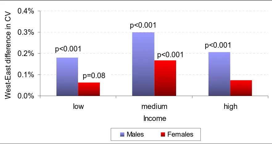
(10) Figure 3.6:. Height difference between West and East Germans as a function of town size (1940-69 birth cohorts). Figure 3.7:. Height convergence in East and West Germany, 1946-79 to 1976-79 birth cohorts, 88 sub-regions. Figure 3.8:. 68. 69. Regional differences in equality, as measured by the coefficient of variation of height, 1930-79 birth cohorts. 73. Figure 3.9:. Average coefficient of variation by state, 1960-67, 1968-75, and 1976-83. 74. Figure 3.10:. Male-to-female coefficient of variation ratio, by year of birth, East and West Germany. Figure 3.11:. Pre-unification coefficient of variation for height in West and East Germany (1940-69 birth cohorts). Figure 3.12:. 79. West-East difference in the pre-unification coefficient of variation for height as a function of town size (1940-69 birth cohorts). Figure 3.14:. 78. West-East difference in the pre-unification coefficient of variation for height as a function of income (1940-69 birth cohorts). Figure 3.13:. 77. 80. Post-unification coefficient of variation for height in West and East Germany. 81. Figure A3.1: Coefficient of variation for height in West and East Germany, by year of birth Figure 4.1:. Average final heights of American male populations. Figure 4.2:. Height of 20 year old West Point candidates (cm) born 1875-79, by. 94 101. region. 102. Figure 4.3:. Trend in BMI for 20-year old West Point cadets and Citadel students. 103. Figure 4.4:. BMI of 20 year old West Point candidates (cm) born 1875-79, by region. 104.

(11) Figure 4.5:. BMI values of 20-year old West Point cadets and Citadel students born in the 1870s, by region. Figure 4.6:. Weight of West Point cadets and Citadel students born in 1870-85, by age. Figure A4.1: Histograms of regression error terms (plus constant) Figure 5.1:. 105. 106 115. Height and BMI distribution of German males (age 18-22) in 2000 and 2001. 121. Figure 5.2:. Height and BMI of German males as a function of education, 2000/01. 124. Figure 5.3:. Height and BMI of German males as a function of health, 2000/01. 125. Figure 5.4:. Height and selected geographic environmental correlates of German males in 2000 and 2001 by region, rank. Figure 5.5:. 127. BMI and selected geographic environmental correlates of German males in 2000 and 2001 by region, rank. 128. Figure 5.6:. Height of German males in 1906, by region. 130. Figure 5.7:. Male height in Germany 1906 and 2000/2001, by social status and region. Figure 5.8:. Male adult height in Germany, birth cohorts of 1938 to 1976 and of 1981/1982, by region. Figure 5.9:. 131. 132. Average adult height (1938 birth cohort) and increase in average adult height (1938-1982 birth cohorts), by region. 133. Figure 5.10:. Increase in height by region, 1906-1950 and 1951-2000. 134. Figure 5.11:. Male BMI in Germany, birth cohorts of 1938 to 1976 and of 1981/1982. 135. Figure 5.12:. Height and BMI, 1973-76 birth cohorts, by urbanization (selected areas). 136.

(12) Chapter 1: Introduction. 12.

(13) 1.1 The Economics of Height Economists are interested in height for at least four reasons. One reason is that a correlation between heights and wages exists: On average, taller men and women earn more than their shorter peers (Ekwo et al. 1991, Averett and Korenman 1993 and Persico et al. 2004 1 ). Because of that, height is usually an important control variable in any well-specified wage equation 2 . Several explanations for the correlation between heights and wages have been discussed in the literature. For example, it has been suggested that, because of interpersonal dominance derived from height, taller people can extract a premium during wage negotiations (Klein et al. 1972). Additionally, it has been argued that taller workers are preferred by employers because they consider them to be more self-confident and assertive (Martel and Biller 1987). Furthermore, according to Persico et al. (2004), tall adults are also relatively tall during adolescence, and because of that are more likely to participate in high school activities in which they obtain skills that are later rewarded in the labor market. Case and Paxson (2006), finally, suggested that taller people have better cognitive ability, and thus their higher income is a return on human capital. In the first essay, we explore another channel. We show that white high-income parents can nourish their daughters in a way so that they become relatively tall adults. With social mobility being limited, these relatively tall daughters will later, like their parents, earn relatively more, generating – at least in part – the positive correlation between heights and wages for this group.. 1. For a more complete list of references, see Chapter 2 of this dissertation. More recently, Mankiw and Weinzierl (2007) have also argued that because of the correlation, “one must either advocate a tax on height, or […] reject, or at least significantly amend, the conventional Utilitarian approach to optimal taxation”. Their argument is that in optimal taxation theory, a Utilitarian social planner aims to transfer income from high-ability individuals to low-ability individuals, but is not able to distinguish between income earned because of ability and income earned because of effort. Since taxing income discourages effort, the planer is deterred from the fully egalitarian outcome. Only by taxing attributes that are positively correlated with ability – such as height –, the planner can get closer to the optimal solution. Based on simulations, Mankiw and Weinzierl show that the optimal tax on height is substantial. A tall person making $50,000 should pay about $4,500 more in taxes than a short person making the same income.. 2. 13.

(14) Authoritarian regimes such as the former GDR tend to report unreliably conventional standard of living indicators, such as income (von der Lippe, 1996, Feshbach and Friedly 1992, Morgan 1999). Accurate height information, however, is frequently available (Pak 2004). As height reflects not only nature but also nurture, the latter can serve as a proxy for conventional indicators. This is a second reason for why economists are interested in height, which in turn has been used to monitor, for example, the decline in the health of the Soviet population during the last decades of its existence, the condition of Taiwan under Japanese occupation (Olds 2003) as well as the suffering of the Chinese population during Mao-Tse Tung’s ‘Great Leap Forward’ policy of the late 1950s and early 1960s (Komlos and Kriwy 2003). In the second essay, we use height to compare the former GDR to West Germany. We show that before unification, the GDR had a lower but more equally distributed biological standard of living than the West. On average, East Germans were shorter than their West German peers (-0.81 cm for females and -0.50 cm for males); however, their heights were distributed more equally in terms of the coefficient of variation (-0.10% for females and 0.06% cm for males). This finding is in contrast to Komlos and Kriwy (2003) who found on the basis of a different data set that height inequality was about the same. With the adoption of the West’s system following re-unification, East Germany rapidly caught up in terms of efficiency (heights), but also in terms of inequality. This implies that a trade-off exists between efficiency and equality not only for conventional indicators (as has often been shown to be the case) but also for the biological standard of living. For most of human history, conventional indicators of living standards are not available at all. National accounts, for example, were only developed during the Great Depression of the 1930s (Ruggles 1983). Information on height, on the other hand, is available as far back. 14.

(15) the 18th century 3 . Many hundreds of thousand of records from nearly all continents of the globe have been examined by now (Komlos 1991). One of the most striking findings of this research is that adult stature in the United States began to decline among the birth cohorts of the 1830s and recovered only in the 1860s. This is surprising and puzzling because according to conventional indicators the American economy was expanding rapidly during the antebellum decades (Komlos 1987, Gallman 1966). In the third paper, we use archival data on West Point cadets born just subsequent to this period in 1860-84 in order to examine the timing and the characteristics of the recovery process. We find that West Point cadets born in the 1880s were taller than those born in the 1860s (+1.46 cm) and had significantly higher BMI values (+0.85). The cadets were on average under-nourished by modern standards, with today’s average reference values being about 5 BMI units higher than those of the cadets. Well-being is inherently multidimensional, encompassing more than the mere command over goods and services (Komlos and Snowdon, 2005). Even today, height can thus contribute to a more nuanced view of the quality of life by documenting developments above and beyond the material well being of a population. This is a fourth reason why economists are interested in height. In the fourth paper, we examine the height and weight of 320,000 German 18-22 year old conscripts born between 1979 and 1982. We find that height is associated with socio-economic differences such as education. A West-East and a North-South gradient in both height and BMI is found. Today, German recruits are about 5 cm taller than their peers 40 years ago and about 12.5 cm taller than those 100 years ago, reflecting a substantial improvement in the biological standard of living. To this day, however, individuals of high socio-economic status are able to reach an above-average height.. 3. In general, the sources are surviving military records. Armies all over the world tended to record the height of their recruits. Similarly, some universities also collected biometric data of their students (e.g. Harvard University for parts of the 19th century, Roche, 1979). 15.

(16) 1.2 References Averett, S. and Korenman, S. (1993). “The Economic Reality of the Beauty Myth.” Journal of Human Resources 31: 304-30. Case, A. and Paxson, C. (2006). “Stature and Status: Height, Ability, and Labor Market Outcomes”, NBER Working Paper No. 12466. Ekwo, E., Gosselink, C., Roizen, N. and Brazdziunas, D. (1991). “The effect of height on family income.“ American Journal of Human Biology 3: 181-88. Feshbach, M. and Friedly, A. (1992). “Ecocide in the USSR: Health and Nature under Siege.” Harper Collins, New York. Gallman, R.E. (1966). “Gross National Product in the United States, 1834-1909.” In Output, Employment, and Productivity in the United States After 1800. New York: National Bureau of Economic Research. Klein, R. E., Freeman, H. E., Kagan, J., Yarbrough, C. and Habicht, J.P. (1972). “Is big smart? The relation of growth to cognition.” Journal of Health and Social Behavior 13: 219-25. Komlos, J. (1991). “On the Significance of Anthropometric History.” Revista di Storia Economica 11: 97-111. Komlos, J. and Kriwy, P. (2003). “The Biological Standard of Living in the Two Germanies.” German Economic Review 4: 493-507. Komlos J. and Lauderdale, B.E. (2007). “Spatial Correlates of U.S. Heights and BMIs, 2002.” Journal of Biosocial Science 39: 59-78.. 16.

(17) Komlos, J. and Snowdon, B. (2005). “Measures of Progress and Other Tall Stories.” World Economics 6: 87-135. Lippe, P. von der (1996). “Die politische Rolle der amtlichen Statistik in der ehemaligen DDR”, Jahrbücher für Nationalökonomie und Statistik 215: 641-73. Mankiw, N.G. and Weinzierl, M (2007). “The Optimal Taxation of Height: A Case Study of Utilitarian Income Redistribution.“, unpublished. Martel, L.F. and Biller, H.B. (1987). “Stature and Stigma: The Biopsychosocial Development of Short Males.” Lexington, Mass.: Lexington Books. Morgan, S. (1999). “Biological Indicators of change in the standard of living in China during the 20th century.” In: Komlos, J. and Baten, J., ed., “The Biological Standard of Living in Comparative Perspective.” Vol. 1. Stuttgart: Franz Steiner. Olds, K. (2003). “The Biological Standard of Living in Taiwan under Japanese Occupation.” Economics and Human Biology 1: 1-20. Pak, S. (2004). “The biological standard of living in the two Koreas.” Economics and Human Biology 2: 511-18. Persico, N., Postlewaite, A. and Silverman, D. (2004). “The Effect of Adolescent Experience on Labor Market Outcomes: The Case of Height.” Journal of Political Economy 112: 1019-53. Roche, A.F. (1979). “Secular Trends in Stature, Weight, and Maturation.” Monographs of the Society for Research in Child Development 44: 3-27. Ruggles, N.D. (1987). "Social accounting," The New Palgrave: A Dictionary of Economics, pp. 377-82.. 17.

(18) Chapter 2: The Correlation between Height and Wages, a Conundrum Explored. 18.

(19) 2.1 Abstract Taller workers earn more. We argue that this is in part because high-income parents can provide sufficient nourishment for their children so that they become relatively tall adults. With limited social mobility, relatively tall children subsequently, like their parents, earn more than average, generating - at least in part - the positive association between height and income. We test this hypothesis by regressing the children’s adult height on their parents’ income at the time the former were adolescents. We find evidence for this hypothesis for white females.. 2.2 Introduction That taller workers earn more is well known. A typical estimate for the wage premium is about 2.5% for every additional inch in height among 30 to 40 year old males and about 2.9% for every additional inch in height among 30 to 40 year old females 1 . Much effort has. 1. Persico et al. (2004), using data from the National Longitudinal Survey of Youth 79, show for the US that. every additional inch in adult height is associated with a 2.5% increase in wages at age 31 to 38 for white male workers. Case and Paxson (2006), using data from the National Health Information Survey, estimate that every additional inch in adult height is associated with a 2.9% increase in wages at age 33 for females. Also for the US, Behrman and Rosenzweig (2001), using data from the Minnesota Twin Registry and exploiting the variation in height between monozygotic twins, estimate that every additional inch in adult height is associated with a 1.7% increase in wages for female workers. Judge and Cable (2004) report that an individual who is 72 inch tall could be expected to earn $5,525 more per year than someone who is 65 inch tall, even after controlling for gender, weight, and age. For the UK, Case and Paxson (2006), using the 1970 cohort of the National Cohort Study, estimate that every additional inch in adult height is associated with a 1.5% increase in wages at age 30 for male workers, and with a 2.8% increase in wages at age 30 for female workers. Heineck (2005), using data from the German Socio-Economic Panel Study, finds that above-average height West German males have gross monthly earnings which are about € 750 higher than those of below-average height West German males. To a lesser extent, the same is true for West German females. Other studies include Averett and Korenman (1993), Cawley (2000), D’Hombres (2007), Ekwo et al. (1991), Heineck (2006), Mirta (2001), Mankiw and Weinzierl (2007), Ribero (2000), Soumyananda et al. (2006), Thomas and Strauss (1997) and in particular Huebler (2006), who finds that the individual height effects on wages are curvilinear rather than linear.. 19.

(20) been made to explain what underlies this empirical relationship: (1) Case and Paxson (2006) suggested that taller people have better cognitive ability, and thus their higher income is a return on human capital. (2) According to Persico et al. (2004), tall adults are also relatively tall during adolescence, and because of that are more likely to participate in high school activities in which they obtain skills that are later rewarded in the labor market. (3) Martel and Biller (1987), Loh (1993) and Magnusson et al. (2006) argue that taller workers are preferred by employers because they consider them to be more self-confident and assertive. (4) Klein et al. (1972), Frieze et al. (1990) and Hensley (1993) suggest that taller people can extract a premium during wage negotiations thanks to interpersonal dominance derived from their height. We propose a complementary reason for the association: higher socio-economic status families nourish their children better so that they become relatively tall adults, but also endow them with more human capital than average. In such a society the social structure reproduces itself with limited social mobility, and the relatively tall children earn more than average, thus generating - at least in part - the positive association between height and income. This hypothesis is not meant as a substitute for the other explanations mentioned above but rather as an additional reason why taller people usually earn a greater income. The inquiry is thus based on two assumptions – social mobility being limited, and high-income parents being able to nourish their children in a way so that they become relatively tall. We do not test whether social mobility is limited, as this issue has already been studied extensively. According to research by Blanden (2005), Perruci and Wysong (2003) and Wysong and Perrucci (2006), only 9% of sons whose fathers were in the lowest quartile of the income distribution ended up in the top quartile during the second half of the 20th century in the US 2 . Some authors even suggest that over recent years, social mobility has become. 2. See also Borjas (1992, 1994), Bowles and Gintis (2004), Menchik (1979), Mulligan (1996), Neal and Johnson (1996), Solon (1992), Tomes (1981), and Zimmerman (1992), in a wider sense also Blank (1991), Cutler and Katz (1991, 1992), Hanratty and Blank (1990), Lerman and Yitzhaki (1985, 1989, 1991) and Stark et al. (1986).. 20.

(21) more limited. Perucci et al. (2007), partly drawing on data contained in Featherman and Hauser (1978), show that in 1973 49 percent of adults were upwardly mobile compared to only about 30 percent of adults in 1998 3 . Many studies have shown that a relationship between social status and height has existed in all societies and at all times even as far back as the 18th century (Komlos et al. 1992), or even in such unexpected places as the former German Democratic Republic (Komlos and Kriwy 2003). However, data on parental income is mostly unavailable so that current adult income has to be used as a proxy for parental income (Komlos and Lauderdale 2007). A study that does use parental income finds that it is positively correlated with children’s height until about a family income of about $80,000. For example, between an annual family income (for a family of four) of c. $10,000 and $80,000 the height of a 17-year-old increases by nearly one inch (2.3 cm) and the height of whites is considerably more sensitive to family income than that of blacks (Komlos and Breitfelder 2007). We explore this relationship further on another data set that contains family income, children’s height, and parental height, examining whether children of wealthier parents attain a higher nutritional status and become relatively tall adults in contemporary America. To do so, we regress adult height of children on the income of their parents during the time the children were adolescents. As a control variable, we use parental height.. 2.3 Data We use data from the National Longitudinal Survey of Youth 97 (NLSY 97) collected by the Bureau of Labor Statistics of the US Department of Labor and designed to gather information on significant life events in a sample of the US population. It is a nationally representative sample of 8,984 youth who were 12 to 16 years old as of December 31, 1996. The 3. See also Schmitt (2005). The evidence on change in the extent of social mobility is disputed (see Solon and Lee. 21.

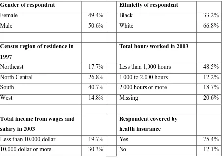
(22) respondents were interviewed every year since then. The NLSY 97 includes information not only on height and wage of the respondents but parental income and height as well. All in all, we use 25 variables from the NLSY 97. Table A2.1 of the appendix lists the variables together with their NLSY identification code. Table 2.1 presents descriptive statistics for the most important variables. Four response items – “total income from wages and salary in 2003”, “parental household income in 1998”, “height of mother”, and “height of father” – have a large share of missing values (50.0%, 72.7%, 25.7 and 50.7%, respectively, see Table 2.1). This is partly because the questions are not applicable to all respondents (i.e. not all individuals have already worked in 2003 at age 18-24, for example) and partly because the NLSY does not pose all questions to all individuals. The data set can be accessed at the NLSY website (http://www.bls.gov/nls/nlsy97.htm).. Table 2.1: Characteristics of the NLSY sample Gender of respondent. Ethnicity of respondent. Female. 49.4%. Black. 33.2%. Male. 50.6%. White. 66.8%. Census region of residence in. Total hours worked in 2003. 1997 Northeast. 17.7%. Less than 1,000 hours. 48.5%. North Central. 26.8%. 1,000 to 2,000 hours. 12.2%. South. 40.7%. 2,000 hours or more. 18.7%. West. 14.8%. Missing. 20.6%. Total income from wages and. Respondent covered by. salary in 2003. health insurance. Less than 10,000 dollar. 19.7%. Yes. 75.4%. 10,000 dollar or more. 30.3%. No. 12.1%. 2006, Mayer and Lopoo 2005, and Levine and Mazumder 2002).. 22.

(23) Missing. 50.0%. Missing. Respondent visited a doctor for. Respondent lived in urban. routine check-up in the last. area in 1997. 12.5%. two years Yes. 71.7%. Yes. 22.6%. No. 12.0%. No. 73.3%. Missing. 16.3%. Missing. Height of mother. 4.1%. Height of father. Between 4 and 5 feet. 2.4%. Between 4 and 5 feet. 0.1%. Between 5 and 6 feet. 70.7%. Between 5 and 6 feet. 34.0%. Between 6 and 7 feet. 1.2%. Between 6 and 7 feet. 15.2%. Other or Missing. 50.7%. Other or Missing. 25.7%. Age at 2003 interviews. Age at 1998 interviews. 18 years old. 0.6%. 13 years old. 0.6%. 19 years old. 14.7%. 14 years old. 15.5%. 20 years old. 15.7%. 15 years old. 16.4%. 21 years old. 15.2%. 16 years old. 16.6%. 22 years old. 15.2%. 17 years old. 17.0%. 23 years old. 12.7%. 18 years old. 13.9%. 24 years old. 0.9%. 19 years old. 1.2%. Missing. 5.7%. Missing. 11.8%. Years of education, residential. Years of education, residen-. mother. tial father. 7 years or less. 5.3%. 7 years or less. 4.3%. 8 years. 2.0%. 8 years. 1.3%. 9 years. 2.9%. 9 years. 2.1%. 10 years. 4.2%. 10 years. 2.2%. 11 years. 5.8%. 11 years. 3.1%. 12 years. 31.9%. 12 years. 21.3%. 23.

(24) 13 years. 7.1%. 13 years. 3.8%. 14 years. 11.1%. 14 years. 8.0%. 15 years. 2.8%. 15 years. 1.8%. 16 years. 10.0%. 16 years. 8.7%. 17 years. 1.8%. 17 years. 1.3%. More than 17 years. 4.2%. More than 17 years. 5.5%. Missing. 10.8%. Missing. 36.5%. Parental household income in 1998 Less than 10,000 dollar. 6.6%. 10,000 to 49,999 dollar. 7.3%. 50,000 to 100,000 dollar. 10.5%. More than 100,000 dollar. 3.0%. Missing/Not part of sub-sample. 72.6%. Note: Number of observations is 5,936. Respondent heights are reported in Figures 2.1-2.4. Source: NLSY 97.. To avoid confounding the effects of race and gender discrimination, Persico et al. (2004) focus on white men only. We use a similar strategy. In a first step, we restrict our sample to those 5,936 respondents who were born in the US and who are classified as either black or white 4 . In a second step, we then run separate regressions by race and gender for these individuals. A limitation of our data is that height is self-reported to the nearest inch. The resulting measurement error is to some extent even evident in the data. For example, about 13% of white females (N=2,932) and 2% of white males (N=3,004) report an adult height that is less than what they reported at age 14, with the error being in the range of one inch in about 85%. 4. This relatively large decline in the number of observations is due to the fact that minorities are over-sampled in. the NLSY 97.. 24.

(25) of cases (Figure 2.1; observations below the 45 degree line reflect an adult height that is less than what the respondent reported at age 14).. Figure 2.1: Scatter diagram between height at age 14 and adult height for white, US-born individuals. 55. 60. Adult height 65. 70. 75. Females. 55. 60. 65 Height at age 14. 70. 75. 25.

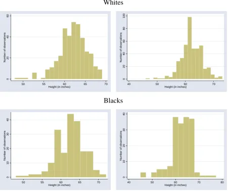
(26) 50. 55. 60. Adult height 65 70. 75. 80. 85. Males. 50. 55. 60. 65 Height at age 14. 70. 75. 80. Note: The sample is restricted to respondents who were 14 years old at the time of the 1997 survey round. Adult height is defined as height at the time of the 2003 survey round when the respondents shown in the diagram were approximately 20 years old. The line shown in the diagram is a 45 degree line. Observations below this line imply that the individual has reported an adult height that is strictly less than what they reported at age 14. Source: NLSY 97.. After controlling for gender, age, and race, height should be distributed normally. In our data, this is not the case for younger respondents, pointing to some misreporting (Figure 2.2). The D'Agostino et al. (1990) and Royston (1991) skewness and kurtosis tests reject the null of normality for all distributions (p<0.01 in all cases, N=382, N=397, N=223 and N=245 respectively) 5 . However, the adult height distributions are normally distributed for whites (Figure 2.3, p=0.2 for females and 0.3 for males) and nearly normal for blacks (p=0.1 for females and males, N=1,959, N=2006, N=974 and N=997, respectively).. 5. While height is generally assumed to be normal for adults of a specific race and gender, it is not entirely clear whether this is also true for children, where different growth tempos may lead to distortions.. 26.

(27) Figure 2.2: Histogram of female (left panel) and male (right panel) height, 14year old, US-born individuals. 0. 0. 20. Number of observations 20 40. Number of observations 40 60 80. 60. 100. Whites. 50. 55. 60 Height (in inches). 65. 70. 40. 50. 60 Height (in inches). 70. 0. 0. 10. Number of observations 20 30. Number of observations 10 20 30. 40. 40. Blacks. 50. 55. 60 Height (in inches). 65. 70. 40. 50. 60 Height (in inches). 70. 80. Note: Height is measured at the time of the 1997 interview. Source: NLSY 97.. 27.

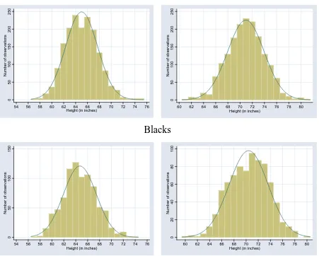
(28) Figure 2.3: Histogram of female (left panel) and male (right panel) adult height, US-born individuals only. 0. 0. 50. 50. Number of observations 100 150 200. Number of observations 100 150 200. 250. 250. Whites. 54. 56. 58. 60. 62. 64 66 68 Height (in inches). 70. 72. 74. 76. 60. 62. 64. 66. 68 70 72 74 Height (in inches). 76. 78. 80. 100 0. 0. 20. Number of observations 50 100. Number of observations 40 60 80. 150. Blacks. 54. 56. 58. 60. 62. 64 66 68 Height (in inches). 70. 72. 74. 76. 60. 62. 64. 66. 68 70 72 Height (in inches). 74. 76. 78. 80. Note: Adult height is height of the respondents at the time of the 2003 interview. Source: NLSY 97.. In the National Health and Nutritional Examination Survey 1999-2004 (NHANES 1999-2004) height is carefully measured 6 . This data set has been recently examined by Komlos and Breitfelder (2006) and in Figure 2.4 we use their growth profiles as benchmark (N=9,965). Average deviation is 0.5 inches (1.32 cm) for white females, 0.78 inches (1.98 cm) for white males, 0.91 inches (2.31 cm) for black females and 0.97 inches (2.46 cm) for black males.. 28.

(29) Figure 2.4: Comparison of NLSY 97 and NHANES 1999-2004 growth profiles, US-born individuals only. 68. 172.7. 66. 167.6. 64. 162.6. 62. 157.5. 60. 152.4. 58. 147.3. 56. height (cm). height (inches). White females. 142.2 12. 13. 14. 15. 16. 17. 18. 19. 20. age NLSY 97. NHANES 1999-2004. 72. 182.9. 70. 177.8. 68. 172.7. 66. 167.6. 64. 162.6. 62. 157.5. 60. 152.4. 58. 147.3. 56. height (cm). height (inches). White males. 142.2 12. 13. 14. 15. 16. 17. 18. 19. 20. age NLSY 97. NHANES 1999-2004. 6. One might ask why we do not use this data set in the first place. The answer is that the NHANES data set does not include information on parental height and parental income while the child grew up. These variables are, however, key to our analysis.. 29.

(30) 68. 172.7. 66. 167.6. 64. 162.6. 62. 157.5. 60. 152.4. 58. 147.3. 56. 142.2 12. 13. 14. 15. 16. 17. 18. 19. height (cm). height (inches). Black females. 20. age NLSY 97. NHANES 1999-2004. 72. 182.9. 70. 177.8. 68. 172.7. 66. 167.6. 64. 162.6. 62. 157.5. 60. 152.4. 58. height (cm). height (inches). Black males. 147.3 12. 13. 14. 15. 16. 17. 18. 19. 20. age NLSY 97. NHANES 1999-2004. Note: NLSY 97 data is on a monthly basis, while the NHANES 1999-2004 data is on an annual basis. Source: NLSY 97, Komlos and Breitfelder (2006).. The NLSY profiles in Figure 2.4 are closer to the NHANES profiles for ages 17-20 than for ages 12-16 in all cases. Given this evidence, it seems safer to focus on adult height. 30.

(31) than on teenage height. Teenage heights, which nonetheless may provide some important insights, must await future research.. 2.4 The relationship between height and wages in the NLSY 97 Like Persico et al. (2004), we regress the log hourly wage of US-born individuals who worked 1,000 hours or more in 2004 on height (Table 2.2) 7 . Age ranges from 19 to 24. We find a significant positive association between heights and wages only for white females (Table 2.2, column 1). For them, one additional inch in height is associated with a 1% increase in the wage. Together with some measurement error, the relatively small number of observations may partly explain why no significant association exists for the other groups studied. Alternatively, it is also possible that many tall, high-potential individuals are in college at age 19-24. This might also explain why the white female wage premium is relatively small when compared to prior estimates.. Table 2.2: OLS estimates, dependent variable: log hourly wage of US-born individuals who worked 1,000 hours or more in 2004, age 19-24 Females. Height. Constant. Adjusted R-squared. Males. White. Black. White. Black. 0.01***. 0.00. -0.00. -0.00. (0.00). (0.00). (0.00). (0.00). 9.25***. 9.50***. (0.20). (0.17). (0.09). (0.21). 0.01. 0.00. 0.00. 0.02. 10.04*** 10.06***. 7. Results are robust for adults who worked more than 1,500 or more than 2,000 hours (tables omitted). Also following Persico et al., we do not include in our models the usual Mincer (1974) control variables - schooling, experience, squared experience. These variables “are endogenous, that is, choice variables that may be influenced by height. This approach [i.e. leaving out the endogenous variables] is consistent with the strategy taken by Neal and Johnson (1996), who, along with Heckman (1998), provide detailed arguments against accounting for differencesin decision variables when estimating the effect of labor market discrimination.” (Persico et al. 2004).. 31.

(32) F-statistic Number of observations. 7.3***. 2.3. 0.5. 1.5. 476. 157. 623. 161. Note: Dependent variable is the log hourly wage at the time of the 2004 interview when respondents were aged 19-24. Observations below the federal minimum wage were deleted. The sample is restricted to individuals who worked 1,000 hours or more. Height is taken from 2004 and measured in inches. Heteroscedasticity-robust Huber-White (1967, 1980) standard errors are in parenthesis. Source: NLSY 97. * significant at 10%; ** significant at 5%; *** significant at 1%. 2.5 Parental income during adolescence and adult height To test our hypothesis, we regress the height of adults on both gross household income of parents during adolescence and parental height (Table 2.3). The model has a number of useful econometric properties. Firstly, misreported heights are less of a problem if height is used as the dependent variable. Provided that the measurement error is not correlated with any of the independent variables, coefficients can be expected to be unbiased (Wooldridge 2005 and Schneeweiss et al. 2006). Secondly, simultaneity is not an issue in this case. Causality runs only from parental income to adolescent height but not the other way round. We thus do not depend on, often imperfect, instrumental variables for identification. Finally, with parental height in the regression equation, the main potential source of omitted variable bias is eliminated.. Table 2.3: OLS estimates, dependent variable: adult height of US-born individuals, age 19-24 Females. Males. White. Black. White. Black. Gross household income of parents during. 0.68**. -0.14. 0.00. -0.18. adolescence, 1998 (in 100,000 dollars). (0.32). (0.10). (0.34). (1.38). 0.36***. 0.25*. 0.44***. 0.31**. Height of mother. 32.

(33) Height of father. Constant. Adjusted R-squared F-statistic Number of observations. (0.06). (0.13). (0.07). (0.14). 0.30***. 0.34***. 0.36***. 0.31**. (0.05). (0.12). (0.06). (0.12). 20.47***. 25.33***. (5.35). (10.78). (6.49). (10.32). 0.35. 0.24. 0.35. 0.20. 26.8***. 5.0***. 23.2***. 5.9**. 212. 54. 201. 35. 17.16*** 28.73***. Note: Dependent variable is height at the time of the 2004 interview when respondents were adults aged 19-24. Height is measured in inches. Gross household income of parents is for 1998 when respondents were still growing. Height of parents is in inches and refers to the height of biological parents. Heteroscedasticity-robust HuberWhite (1967, 1980) standard errors are in parenthesis. Source: NLSY 97. * significant at 10%; ** significant at 5%; *** significant at 1%. For white females, the coefficient is significantly positive at the 5% level (Table 2.3, column 1). An increase in yearly parental gross household income by $100.000 leads to an increase in the adult height of children of 0.68 inches (1.73 cm). On average, daughters of low-income ($20,000) parents reach an adult height of 65.3 inches (165.9 cm), while those of medium-income ($49,000) parents reach an adult height of 65.5 inches (166.4 cm), and those of high-income ($78,000) parents reach an adult height of 65.7 inches (166.9 cm) (Figure 2.5). If social mobility is limited, these relatively tall children will later, like their parents, earn more relative to their shorter peers, generating in part the positive association between height and income 8 . The “parental income height premium” exists only for females. This makes sense given that most of the other explanations discussed in the introduction pertain to men only while the height premium is actually comparable in size for males and females. There is also evidence from historical studies that shows that the height of females reacts. 8. The result is robust to gross household income being used in logarithmic form.. 33.

(34) stronger to an exogenous shock in the biological standard of living than male height (Sunder 2007).. 65.8. 167.1. 65.7. 166.9. 65.6. 166.6. 65.5. 166.4. 65.4. 166.1. 65.3. 165.9. 65.2. 165.6. 65.1. 165.4 low. medium. adult height (in cm). adult height (in inches). Figure 2.5: Average adult height of white US-born females with parents of average height as a function of parental yearly gross household income during adolescence. high. parental income during adolescence. Note: The figure is based on the regression results of Table 2.3, column 1. In the figure, a low (medium, high) parental income during adolescence is defined as an income of $20,000 ($49,000; $78,000). The effect of parental income during adolescence is significant at the 5% level. Source: NLSY 97.. 2.6 Channels Why parental income influences female height is not obvious, given that the food budget is a relatively small part of total expenditures today. To learn more about the transmission channels, our data set affords a rich set of variables. In a first step, we add a dummy variable for whether a respondent visited a doctor for a routine check-up in the last two years. Children, who did not see a doctor for a routine check-. 34.

(35) up in the last two years are on average about 1.33 inch (3.4 cm) shorter than children who have visited a doctor for a routine check-up in the last two years (column 1 of Table 2.4 and Figure 2.6). The coefficient on income of parents is reduced from 0.68 to 0.64, suggesting that about 6% of the parental income height premium can be explained by being able to make doctor visits. The generally good education of high-income parents might also help their children in becoming relatively tall, for example, because they can weigh better the risks associated with neglecting doctor visits. We control for this by adding the educational achievement of the mother and the father (Table 2.4, column 2). Unlike our control for health consciousness, parental education is not significant in this model 9 . Adding dummy variables for the four US Census regions reduces the coefficient of interest by more than 10% to 0.59 (column 3 of Table 2.4) 10 . While self-selection (some regions may attract high-income and tall people with, for genetic reasons, tall children) may explain part of the result, this nevertheless suggests that the “parental income height premium” is partly transmitted by high-income parents living in regions where their children have better access to advanced medical facilities, clean air and fresh fruit, all of which help growth as height depends positively on gross nutritional intake and negatively on claims on the human body such as illness (Komlos 1989). Adding controls for whether a respondent lives in an urban or rural area also mediates the initial parental income height premium (-6% to 0.65, column 4 of Table 2.4). If all variables discussed so far are included in the model, the initial coefficient on income (column 1) is reduced by about 20% (column 5 of Table 2.4) 11 .. 9. Results are qualitatively unchanged if we control only for mother’s or father’s education. Only if we leave out parental income and parental height, does education have the expected positive effect. The same is true when we add controls for the education of the respondent herself/himself instead of controls for the education of parents (results omitted). 10 Information on the composition of the four Census regions (Northeast, North Central, South and West) is contained in Figure A2.1 in the Appendix. 11 There are other channels that might be worth exploring. Studies show that cost is the most significant predictor of dietary choice (Foley and Pollard 1998, Mackerras 1997). Hence, poorer people consume cheaper food, which may also be less healthy. Furthermore, poor neighborhoods in the U.S. have limited access to supermarkets, which offer a wide variety of healthy food (Morland et al. 2002), making dietary change difficult to achieve. Smoking parents, no health insurance, little social safety and psychosocial stress may also adversely affect the height of children (Fogelman and Manor 1988, Sunder 2003, Steckel 2008, Woitek 2003, Sunder and Woitek. 35.

(36) Table 2.4: OLS estimates, dependent variable: adult height of white US-born females, age 19-24 (1). (2). (3). (4). (5). Gross household income of parents. 0.64**. 0.65*. 0.59*. 0.65*. 0.55. during adolescence (in 100,000. (0.32). (0.35). (0.32). (0.33). (0.36). 0.36***. 0.36***. 0.36***. 0.36***. 0.36***. (0.06). (0.06). (0.06). (0.06). (0.06). 0.30***. 0.30***. 0.30***. 0.30***. 0.30***. (0.05). (0.05). (0.05). (0.05). (0.05). dollars) Height of mother. Height of father. Respondent has not visited a doctor for a routine check-up in the last. -1.33**. -1.25*. (0.62). (0.65). two years Respondent has visited a doctor for Reference. Reference. a routine check-up in the last two years Years of education, mother. Years of education, father. South Northeast. North Central. West. Rural. Urban. -0.02. -0.02. (0.07). (0.07). 0.03. 0.01. (0.07). (0.07) Reference 0.39. 0.33. (0.53). (0.54). 0.51. 0.47. (0.37). (0.34). 0.18. 0.05. (0.43). (0.49) -0.07. -0.25. (0.92). (0.93). 0.11. -0.01. (0.92). (0.91). 2005, Wadsworth et al. 2002, Peck and Lundberg 1995, Montgomery et al. 1997, Silventoinen et al. 1999, Davey-Smith et al. 2000 ). Due to small sample size, we can not examine these channels with our own data in a meaningful way.. 36.

(37) Other than rural or urban Constant. Reference Reference 20.33*** 20.35*** 20.44*** 20.10*** 20.18***. Adjusted R-squared F-statistic Number of observations. (5.36). (5.53). (5.40). (5.51). (5.71). 0.32. 0.31. 0.32. 0.31. 0.31. 21.3***. 16.4***. 13.0***. 16.2***. 7.7***. 212. 212. 212. 212. 212. Note: Dependent variable is height at the time of the 2004 interview when respondents were adults aged 19-24. Height is measured in inches. Gross household income of parents is for 1998 when respondents were still growing. Height of parents is in inches and refers to the height of biological parents. Heteroscedasticity-robust HuberWhite (1967, 1980) standard errors are in parenthesis. Source: NLSY 97. * significant at 10%; ** significant at 5%; *** significant at 1%. 66.5. 168.9. 66.0. 167.6. 65.5. 166.4. 65.0. 165.1. 64.5. 163.8. 64.0. 162.6 no doctor visits. height (cm). height (inches). Figure 2.6: Average adult height of white US-born females with parents of average height and average income as a function of doctor visits. doctor visits. Note: The figure is based on the regression results of Table 2.4, column 1. The effect is significant at the 5% level. Source: NLSY 97.. 37.

(38) 2.7 Conclusion Several explanations have been offered for why employers pay a wage premium for taller workers. Either taller people have more human capital, or employers have a preference for taller people for managerial positions. We add an additional explanation by arguing that taller people earn more because high-income parents can nourish their children in a way so that they become relatively tall adults. If social mobility is limited, these relatively tall children later earn more, like their parents, generating - at least in part - the positive association between heights and wages. We test this hypothesis by regressing children’s adult height on the income of their parents during the time the former were still growing, controlling for parental height. We find evidence for our hypothesis only for white females. The white female “parental income height premium” is partially mediated through health conscious behavior, parental education and geographical location choice. We show that children who have not visited a doctor for a routine check-up in the last two years are on average about 1.33 inch (3.4 cm) shorter than children who have visited a doctor for a routine check-up in the last two years. This result contributes to the growing literature on the “biological standard of living“ (Floud 1994, Fogel 1994, Komlos 1985, 1989, Steckel 2008, Waaler 1984). According to this literature, conventional standard of living measures should be complemented by measures like health status, body-mass index, longevity, or average height, as “well being encompasses more than just the command over goods and services” (Komlos and Snowdon, 2005). Average height is the variable most often used in this literature. Reflecting the net nutritional status of a population, average height is sensitive to many socio-economic influences. The paper adds to this literature by showing that parental income and health consciousness affect the height of adolescent girls.. 38.

(39) 2.8 References Averett, S. and Korenman, S. (1993). “The Economic Reality of the Beauty Myth.” Journal of Human Resources 31: 304-30. Beard, A.S. and Blaser, M.J. (2002). “The Ecology of Height: The Effect of Microbial Transmission on Human Height.” Perspectives in Biology and Medicine 45: 475-99. Behrman, J. and Rosenzweig, M. (2001). “The Returns to Increasing Body Weight.” Working paper. Philadelphia: University of Pennsylvania. Blanden, J. (2005). “International Evidence on Intergenerational Mobility.” Working Paper, Department of Economics, University College London. Blank, R.M. (1991). “Why Were Poverty Rates So High in the 1980s?” NBER Working Paper 3878. Bobak, M., Kriz, B., Leon, D.A., Danova, J. and Marmot, M. (1994). “Socioeconomic factors and height of preschool children in the Czech Republic.” American Journal of Public Health 84: 1167-70. Borjas, G. (1992). “Ethnic capital and intergenerational mobility.” Quarterly Journal of Economics 107: 123-50. Borjas, G. (1994). “Long-run convergence of ethnic skill differentials: the children and grandchildren of the great migrations.” Industrial & Labor Relations Review 47: 553-73. Bowles, S. and Gintis, H. (2004). “The Inheritance of Inequality.” Journal of Economic Perspectives 16: 3-30. Case, A. and Paxson, C. (2006). “Stature and Status: Height, Ability, and Labor Market Outcomes”, NBER Working Paper 12466.. 39.

(40) Cavelaars, A. E., Kunst, A. E., Geurts, J. J., Crialesi, R., Grotvedt, L., Helmert, U., Lahelma, E., Lundberg, O., Mielck, A., Rasmussen, N. K., Regidor, E., Spuhler, T. and Mackenbach, J. P. (2000). “Persistent variations in average height between countries and between socio-economic groups: an overview of 10 European countries.” Annals of Human Biology 27: 407-21. Cawley, J. (2000). “Body Weight and Women's Labor Market Outcomes.” NBER Working Papers 7841. Cutler, D.M. and Katz, L.F. (1991). “Macroeconomic Performance and the Disadvantaged.“ Brookings Papers on Economic Activity 2: 1-74. Cutler, D.M. and Katz, L.F. (1992). „Rising Inequality? Changes in the Distribution of Income and Consumption in the 1980's.“ The American Economic Review 82: 546-51. D'Agostino, R. B., Balanger, A. and D'Agostino R. B., Jr. (1990). “A suggestion for using powerful and informative tests of normality.” American Statistician 44: 316-21. D'Hombres, B. (2007). “Does body height affect wages?” Economics and Human Biology 5: 1-19. Davey-Smith, G., Hart, C. and Upton, M. (2000). “Height and risk of death among men and women: aetiological implications of associations with cardiorespiratory disease and cancer mortality.” Journal of Epidemiology and Community Health 54: 97-103. Ekwo, E., Gosselink, C., Roizen, N. and Brazdziunas, D. (1991). “The effect of height on family income.“ American Journal of Human Biology 3: 181-88. Floud, R. (1994). “The heights of Europeans since 1750: a new source for European economic history.” In: Komlos, J. (Ed.), Stature, Living Standards, and Economic Development: Essays in Anthropometric History. The University of Chicago Press, Chicago, 9–24.. 40.

(41) Fogel, R.W. (1994). “Economic growth, population theory, and physiology: the bearing of long-term processes on the making of economic policy.” American Economic Review 84: 369–95. Fogelman, K.R. and Manor, O. (1988). “Smoking in pregnancy and development into early adulthood.” British Medical Journal 297: 1233-36. Foley, R.M. and Pollard, C.M. (1998). “Food cent$ - implementing and evaluating a nutrition education project focusing on value for money.” Australian and New Zeeland Journal of Public Health 22: 494-501. Frieze, I.H., Olson, J.E. and Good, D.C. (1990). “Perceived and Actual Discrimination in the Salaries of Male and Female Managers.” Journal of Applied Social Psychology 20: 4667. Hanratty, M.J. and Blank, R.M. (1990). “Down and Out in North America: Recent Trends in Poverty Rates in the U.S. and Canada.” NBER Working Papers 3462. Heckman, J.J. (1998). “Detecting Discrimination.” Journal of Economic Perspectives 12: 101-16. Heineck, G. (2005). “Up in the skies? The relationship between height and earnings in Germany.” Labour: Review of Labour Economics and Industrial Relations 19: 469-89. Heineck, G. (2006). “Height and weight in Germany, Evidence from the German Socio-Economic Panel, 2002.” Economics and Human Biology 4: 359-82. Hensley, W.E. (1993). “Height as a Measure of Success in Academe.” Psychology, Journal of Human Behavior 30: 40-46.. 41.

(42) Huber, P. J. (1967). “The behavior of maximum likelihood estimates under nonstandard conditions.” Proceedings of the Fifth Berkeley Symposium on Mathematical Statistics and Probability. Berkeley, CA: University of California Press, vol. 1: 221-23. Huebler, O. (2006). “The Nonlinear Link between Height and Wages: An Empirical Investigation.” IZA Discussion Papers 2394. Institute for the Study of Labor (IZA). Bonn. Judge, T.A. and Cable, D.M. (2004). “The Effect of Physical Height on Workplace Success and Income: Preliminary Test of a Theoretical Model.” Journal of Applied Psychology 89: 428-41. Klein, R. E., Freeman, H. E., Kagan, J., Yarbrough, C. and Habicht, J.P. (1972). “Is big smart? The relation of growth to cognition.” Journal of Health and Social Behavior 13: 219-25. Kleinman, J.C. and Madans, J.H. (1985). “The effects of maternal smoking, physical stature, and educational attainment on the incidence of low birth weight.” American Journal of Epidemiology 121: 843-55. Komlos, J. (1985). “Stature and Nutrition in the Habsburg Monarchy: The Standard of Living and Economic Development.” American Historical Review 90: 1149-61. Komlos, J. (1989). “Nutrition and economic development in the eighteenth century Habsburg monarchy.” Princeton: Princeton University Press. Komlos, J. (1991). “On the Significance of Anthropometric History.” Revista di Storia Economica 11: 97-111. Komlos, J. and Breitfelder, A. (2006). “Improvements in the most recent CDC height growth charts for the US.” Unpublished.. 42.

(43) Komlos, J. and Breitfelder, A. (2007). “The height of US-born non-Hispanic children and adolescents ages 2-19, born 1942-2002 in the NHANES Samples.” American Journal of Human Biology, forthcoming. Komlos, J. and Kriwy, P. (2003). “The Biological Standard of Living in the Two Germanies.” German Economic Review 4: 493-507. Komlos, J. and Lauderdale, B.E. (2007). “Underperformance in Affluence: the Remarkable relative decline in American Heights in the second half of the 20th-Century.” Social Science Quarterly 88: 283-304. Komlos, J. and Snowdon, B. (2005). “Measures of Progress and Other Tall Stories.” World Economics 6: 87-135. Komlos, J., Tanner J.M., Davies P.S.W. and Cole, T. (1992). “The Growth of Boys in the Stuttgart Carlschule, 1771-93.” Annals of Human Biology 19: 139-52. Lerman R.I. and Yitzhaki, S. (1985). “Income Inequality Effects by Income Source: A New Approach and Applications to the United States.” The Review of Economics and Statistics 67: 151-56. Lerman R.I. and Yitzhaki, S. (1989). “Improving the accuracy of estimates of Gini coefficients," Journal of Econometrics 42: 43-47. Lerman R.I. and Yitzhaki, S. (1991). “Income Stratification and Income Inequality.” Review of Income and Wealth 37: 313-29. Levine, D.I. and Mazumder, B. (2002). “Choosing the right parents: changes in the intergenerational transmission of inequality between 1980 and the early 1990s,” Working Paper Series WP-02-08, Federal Reserve Bank of Chicago.. 43.

(44) Lindgren, G. (1976). “Height, weight and menarche in Swedish urban school children in relation to socio-economic and regional factors.” Annals of Human Biology 3: 501-28. Loh, E.S. (1993). “The Economic Effects of Physical Appearance.” Social Science Quarterly 74: 420-38. Mackerras, D. (1997). “Disadvantaged and the cost of food.” Australian and New Zeeland Journal of Public Health 21: 218. Magnusson, P.K.E., Rasmussen, F. and Gyllensten, U.B. (2006). “Height at Age 18 Years is a Strong Predictor of Attained Education Later in Life: Cohort Study of Over 950000 Swedish Men.” International Journal of Epidemiology 35: 658-63. Mankiw, N.G. and Weinzierl, M. (2007). “The Optimal Taxation of Height: A Case Study of Utilitarian Income Redistribution.“, unpublished. Martel, L.F. and Biller, H.B. (1987). “Stature and Stigma: The Biopsychosocial Development of Short Males.” Lexington, Mass.: Lexington Books. Mayer, S.E. and Lopoo, L.M. (2005). “Has the Intergenerational Transmission of Economic Status Changed?” Journal of Human Resources 40: 169-185. Menchik, P.L. (1979). “Inter-generational transmission of inequality: an empirical study of wealth mobility.” Economica 46: 349-62. Mincer, J. (1974). “Schooling, Experience and Earnings.” New York: National Bureau of Economic Research. Mirta, A. (2001). “Effects of Physical Attributes on the Wages of Males and Females.” Applied Economics Letters 8: 731-35. Montgomery, S., Bartley, M. and Wilkinson, R. (1997). “Family conflict and slow growth.” Archives of Disease in Childhood 44: 326-30. 44.

(45) Morland, K., Wing, S., Diez Roux, A. and Poole, C. (2002). “Neighborhood characteristics associated with the location of food stores and food service places.” American Journal of Preventive Medicine 22: 23-29. Mulligan, C.B. (1996). “Parental Priorities and Economic Inequality.” Chicago: University of Chicago Press, forthcoming. Neal, D.A. and Johnson, W.R. (1996). “The role of premarket factors in black-white wage differences.” Journal of Political Economy 104: 869-95. Peck, M. and Lundberg, O. (1995). “Short stature as an effect of economic and social conditions in childhood.” Social Science and Medicine 41: 733-38. Peck, A. M. and Vagero, D.H. (1987). “Adult body height and childhood socioeconomic group in the Swedish population.” Journal of Epidemiology and Community Health 41: 333-37. Perrucci, R. and Wysong, E. (2003). “The New Class Society.” 2nd ed. Landham, Maryland: Rowman and Littlefield. Persico, N., Postlewaite, A. and Silverman, D. (2004). “The Effect of Adolescent Experience on Labor Market Outcomes: The Case of Height.” Journal of Political Economy 112: 1019-53. Ribero, R. (2000). “Adult morbidity, height and earnings in Colombia.” In: Savedoff, W. and Schultz, T.P., ed., “Wealth from Health.” Latin American Research Network. InterAmerican Development Bank. Washington, D.C. Royston, P. (1991). “sg3.5: Comment on sg3.4 and an improved D'Agostino test.” Stata Technical Bulletin 3:19. Reprinted in Stata Technical Bulletin Reprints 1: 110-12.. 45.

(46) Schneeweiss, H., Komlos, J. and Ahmad, A.S. (2006). “Symmetric and Assymetric Rounding.” Discussion Paper 479, Sonderforschunsbereich 386, LMU Munich. Silventoinen, K., Lahelma, E. and Rahkonen, O. (1999). “Social background, adult body-height and health.” International Journal of Epidemiology 28: 911-18. Solon, G.R. (1992). “Intergenerational income mobility in the United States.” American Economic Review 82: 393-408. Solon, G.R. and Chul-In, L. (2006). “Trends in Intergenerational Income Mobility.” NBER Working Paper No. W12007. Soumyananda, D., Gangopadhyay, P.K., Chattopadhyay, B.P., Saiyed, H.N., Pal, M. and Bharati, P. (2006). “Height, weight and earnings among coalminers in India.“ Economics and Human Biology 4: 342-50. Stark, O., Taylor, J.E. and Yitzhaki, S. (1986). “Remittances and Inequality.” Economic Journal 96: 722-40. Steckel, R.H. (2008). “Biological Measures of the Standard of Living.” Journal of Economic Perspectives 22: 129-152. Sunder, M. (2003). “The Making of Giants in a Welfare State: The Norwegian Experience in the 20th Century.” Economics and Human Biology 1: 267-76. Sunder, M. (2007). “Passports and Economic Development: An Anthropometric History of the U.S. Elite in the Nineteenth Century.” Unpublished manuscript. University of Munich. Sunder, M. and Woitek, U. (2005). “Boom, Bust, and the Human Body: Further Evidence on the Relationship between Height and Business Cycles.” Economics and Human Biology 3: 450-66. 46.

(47) Thomas, D. and Strauss, J. (1997). “Health and Wages: Evidence on Men and Women in Urban Brazil.“ Papers 97-05, RAND. Tomes, N. (1981). “The family, inheritance, and the intergenerational transmission of inequality.” Journal of Political Economy 89: 928-58. Waaler, H. (1984). “Height, weight, and mortality: the Norwegian experience.” Acta Medica Scandicana (Supplement) 679: 1–56. Wadsworth, M., Hardy, R., Paul A., Marshall, S. and Cole, T. (2002). “Leg and trunk length at 43 years in relation to childhood health, diet and family circumstances; evidence from the 1946 national birth cohort.” International Journal of Epidemiology 31: 383-90. White, H. (1980). “A heteroskedasticity-consistent covariance matrix estimator and a direct test for heteroskedasticity.” Econometrica 48: 817-30. Woitek, U. (2003). Height cycles in the 18th and 19th centuries, Economics and Human Biology 1: 243-57. Wooldridge, J.M. (2005). “Econometric Analysis of Cross Section and Panel Data.” MIT Press. Zimmerman, D.J. (1992). “Regression toward mediocrity in economic stature.” American Economic Review 82: 409-29.. 47.

(48) 2.9 Appendix Table A2.1: Survey year and NLSY code for variables used in the paper No. Variable. Survey. NLSY code. year 1. Height in 1997. 1997. R0322500, R0322600. 2. Height in 1998. 1998. R2164100, R2164200. 3. Height in 1999. 1999. R3482000, R3482100. 4. Height in 2000. 2000. R4880200, R4880300. 5. Height in 2001. 2001. R6497600, R6497700. 6. Height in 2002. 2002. S0905500, S0905600. 7. Height in 2003. 2003. S2978200, S2978300. 8. Height in 2004. 2004. S4677000, S4677100. 9. Total income from wages and salary in 2003. 2004. S4799600. 10. Total hours worked in 2003. 2004. S3817100. 11. Parental household income in 1998. 1998. R2563300. 12. Height of father. 1997. R0608200, R0608300, R0608500, R0608600, R0608900, R0609000. 13. Height of mother. 1997. R0608200, R0608300, R0608500, R0608600, R0608900, R0609000. 14. Gender identification biological parents. 1997. R0733700, R0734200, R0735100, R0734800. 15. Gender of respondent. 1997. R0536300. 16. US-born. 1997. R5821400. 17. Ethnicity of respondent. 1997. R1482600. 18. Exact age during 1998 interview. 1998. R2553400. 19. Exact age during 2003 interview. 2003. S2000900. 20. Years of education, residential father. 1997. R1302600. 21. Years of education, residential mother. 1997. R1302700. 22. Respondent covered by health insurance. 1997. R0686800. 48.

(49) 23. Respondent visited a doctor for routine check-. 2003. S1240500. up in the last two years 24. Respondent lived in urban area in 1997. 1997. R1217500. 25. Census region of residence in 1997. 1997. R1200300. Source: NLSY 97.. Figure A2.1: US Census Regions. Note: Northeast: CT=Connecticut, ME=Maine, MA=Massachusetts, NJ=New Jersey, NH=New Hampshire, NY=New York, PA=Pennsylvania, RI=Rhode Island, and VT=Vermont. North Central: IL=Illinois, IN=Indiana, IA=Iowa, KS=Kansas, MI=Michigan, MN=Minnesota, MO=Missouri, NE=Nebraska, ND=North Dakota, OH=Ohio, SD=South Dakota, and WI=Wisconsin. South: AL=Alabama, AR=Arkansas, DE=Delaware, DC=District of Columbia, FL=Florida, GA=Georgia, KY=Kentucky, LA=Louisiana, MD=Maryland, MS=Mississippi, NC=North Carolina, OK=Oklahoma, SC=South Carolina, TN=Tennessee, TX=Texas, VA=Virginia, and WV=West Virginia. West: AK=Alaska, AZ=Arizona, CA=California, CO=Colorado, HI=Hawaii, ID=Idaho, MT=Montana, NM=New Mexico, NV=Nevada, OR=Oregon, UT=Utah, WA=Washington, and WY=Wyoming. Source: Map by the Indiana Business Research Center, Kelley School of Business, Indiana University.. 49.

(50) Chapter 3: The Trade-off between a High and an Equal Biological Standard of Living – Evidence from Germany. 50.

(51) 3.1 Abstract Following German re-unification, East Germany moved from a state-socialist to a marketbased economic system. Using West Germany as a “control group”, we examine how the change affected the level and the equality of the biological standard of living. We find that before unification, East Germany had a lower but somewhat more equally distributed biological standard of living than the West. After unification, East Germany rapidly caught up in terms of height but at the expense of equality. This suggests that a trade-off exists between a high and an equally distributed biological standard of living. Unlike previous research, we find that West Germany’s pre-unification height advantage was smallest in towns with 5,000 to 20,000 inhabitants and largest in cities with 20,000 to 100,000 inhabitants (females) or in cities with more than 100,000 inhabitants (males). Between regions, height converged both in East and West Germany, but particularly markedly among East German males. Equality convergence, like height convergence, is significantly larger for East than for West German males.. 3.2 Introduction Biological welfare indicators such as health, longevity and height are useful complements to conventional indicators of welfare as they reflect the socioeconomic and environmental circumstances experienced by a population (Bogin, 1999; Floud, 1994; Fogel, 1994; Komlos, 1985, 1989; Steckel, 1995, 2008; Sunder, 2003; Waaler, 1984). As Komlos and Kriwy (2003) point out, this is particularly true for comparisons between countries with different economic and political systems such as the two Germanies prior to unification. After all, in such cases, conventional welfare measures are limited in their usefulness as it is hard to control for differences in the way prices are determined, in the quality and availability of 51.

(52) goods, and in the reliability of official data. Apart from that, it is questionable to what extent conventional indicators can capture all dimensions of the quality-of-life. “How, for example, should one interpret the fact that East German employees earned about half of their Western counterparts in 1980, and their travel was restricted, but had full employment and a more equal distribution of income?” (Komlos and Kriwy 2003). With surveys of contentment also unavailable, biological welfare indicators are useful for comparing well being in East and West Germany before unification (Komlos and Baur 2004 and Heineck 2006). From a social point of view, not only a high but also an equally distributed standard of living is desirable. In Germany, a “just and equal income distribution” is a goal actually mandated by a law enacted in 1963 (Kämper 1992, Krupp 1985, Moeller 1968, Schiller 1978) 1 . It is often suggested that the goals of a high living standard and an equally distributed living standard are to some extent conflicting. As Browning and Johnson (1984) argue: “Income redistribution is not a socially costless endeavor because the policies required to accomplish it generally produce misallocations of resources” (Aghion et al. 1999, Baumol and Fischer 1979, Benabou 1994, 1996, 2000, 2005, Blyth 1997, Lee 1987, 1993, Niggle 1997, 1998, Okun 1975, Persson and Tabellini 1994, Vallentyne 2000; see, however, also Lindert 2007). Empirical evidence for a trade-off between equality and efficiency (in Germany) comes from Hauser (1992), Loetsch (1991, 1993) and Dathe (1998). They show that after unification, average income in East Germany increased together with the number of poor households. In 1990, only 3% of East German households had an income of less than half of the average per capita income. By 1997, about 8% did. Despite much research on the biological standard of living, little is known about to what extent such a trade-off exists.. 1. This makes sense in view of the so called Easterlin Paradox of Happiness Economics, which states that the effectiveness of income as a generator of well-being is greatly diminished once income reaches a certain level (Easterlin 1974). The reason is that aspiration increases along with income and after basic needs are met, relative rather than absolute levels of income become important for well-being (“hedonic treadmill”, Brickman and Campbell 1971, Clark et al. 2006, Diener 2005, Di Tella 2001, 2004, Frank 1997, Frey and Stutzer 2000, 2002, Hepburn and Eysenck 1989, Layard, R. 2005, Phelps 2001, Sen 1970, 1985, 1992, 1995, 1999).. 52.

(53) 3.3 Data The German Mikrozensus is a yearly survey of 1% of households, which is about 370,000 households or about 820,000 persons 2 . For the survey, districts are selected in which all persons are interviewed. The public use files are 70% subsamples of the original Mikrozensus, designed to better ensure the anonymity of respondents. We restrict our analysis to the Mikrozensus rounds 1999 and 2003, as these rounds are the only ones which include a question on the height of respondents. We exclude all implausible observations. For the sake of comparability, we exclude immigrants. Throughout the paper, both rounds of the Mikrozensus are pooled together to increase sample size. Descriptive statistics of the sample are available in Table A3.1 of the Appendix. Since height is self-reported in the Mikrozensus, we should be aware of potential bias. We compare the trend in height calculated from the Mikrozensus data to similar profiles for the 1998 Bundesgesundheitssurvey (BGS, “Federal Health Survey”), in which height is measured by professionals (Stolzenberg 2000). On average, we have 2,003 female observations per annual birth cohort in the Mikrozensus but only 82 in the BGS. For males, the respective numbers are 2,012 and 77. In the Mikrozensus, East and West German female height is on average 0.3 cm above the BGS trend (Figure 3.1) 3 . Deviations are larger for older than for younger individuals (0.7 cm in the West and 0.8 cm in the East at age 50 to 80 versus 0.2 cm and 0.1 cm at age 20 to 49), suggesting that respondents are not fully aware of age-related shrinking. Males show less over-reporting than females. Average deviation is 0.6 cm in the West and 0.5 cm in the East. Again, deviations are larger for older than for younger respondents, though only slightly (0.6 cm at age 50 to 80 and 0.5 cm at age 20 to 49).. 2. The survey is conducted by the Bundesamt für Statistik (Federal Statistical Office) jointly with the statistical offices of the 16 individual German states. Most items in the Mikrozensus questionnaire are subject to compulsory response. The data can be ordered under the following address: http://www.gesis.org/en/social_monitoring/GML/data/mc/index.htm. 3 We refer to people living in regions that once belonged to the German Democratic Republic as East Germans, and to people living in areas that belonged to the Federal Republic of Germany as West Germans.. 53.

(54) Figure 3.1: Comparison of Mikrozensus and Bundesgesundheitssurvey average adult height, by year of birth, East and West Germany Females 186. 180. 184 West Germany left hand scale. 178. 182. 176. 180. 174. 178 East Germany right hand scale. 172. 176. 170. 174. 168. 172. 166. 170 1980. 1975. East MZ. 1970. 1965. West BGS. 1960. 1955. 1950. 1945. 1940. 1935. 1930. West MZ. Height (cm) East Germany. Height (cm) West Germany. 182. East BGS. Males 174. 168. 172. West Germany left hand scale. 166. 170. 164. 168. 162. 166 East Germany right hand scale. 160. 164. 158. 162. 156. 160. 154. 158 1980. 1975. East MZ. 1970. 1965. West BGS. 1960. 1955. 1950. 1945. 1940. 1935. 1930. West MZ. Height (cm) East Germany. Height (cm) West Germany. 170. East BGS. Note: Mikrozensus data is on a yearly basis, while the BGS data reflects 5-year averages. Height in the Bundesgesundheitssurvey is measured by professionals.. 54.

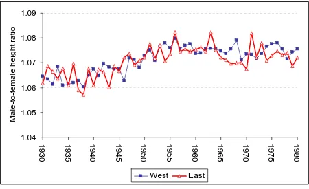
(55) Source: Mikrozensus 1999 and 2003, Bundesgesundheitssurvey 1998. The male-to female height ratio was similar in East and West Germany throughout the period under consideration (Figure 3.2). In both parts of Germany, the male height advantage increased beginning with the birth cohorts of the 1950s.. Figure 3.2: Male-to-female height ratio, by year of birth, East and West Germany. Male-to-female height ratio. 1.09 1.08 1.07 1.06 1.05 1.04 1980. 1975. 1970. 1965. 1960. 1955. 1950. 1945. 1940. 1935. 1930. West. East. Source: Mikrozensus 1999 and 2003. 3.4 Level of the biological standard of living in East and West Germany before and after unification Using the BGS data set, Komlos and Kriwy (2003) showed that, despite their genetic similarity, West Germans were significantly taller than East Germans before unification. They conclude that the mixed economy in the West led to a higher biological standard of living 55.

No results found