TESNAT 2017
a Corresponding author: [email protected]
© The Authors, published by EDP Sciences. This is an open access article distributed under the terms of the Creative Commons Attribution License 4.0 (http://creativecommons.org/licenses/by/4.0/).
Multilinear analysis of Time-Resolved Laser-Induced
Fluorescence Spectra of U(VI) containing natural water samples
Jakub Višňák, 1,5,6,a, Robin Steudtner2, Andrea Kassahun4 and Nils Hoth3
1Dept. of Nuclear Chemistry, FNSPE, Czech Technical University, Břehová 7, 115 19 Prague 1, Czech Rep. 2Institut für Radiochemie, Forschungszentrum Rossendorf e.V., P.O. Box 510119, 01314 Dresden, Germany
3Univ. of Mining and Technology, Dept. of Mining and Special Construction Engineering, Zeunerstr. 1A, 09596 Freiberg, Germany. 4WISMUT GmbH, Jagdschänkenstr. 29, 09117 Chemnitz, Germany.
5Dept. of Chemical Physics and Optics, Faculty of Mathematics and Physics, Charles Univ., Ke Karlovu 3, 121 16 Prague 2, Czech Rep. 6J. Heyrovský Institute of Physical Chemistry, Dolejškova 2155/3, 182 23 Prague 8, Czech Rep.
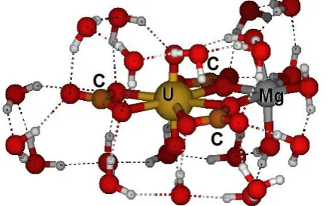
Abstract. Natural waters’ uranium level monitoring is of great importance for health and environmental protection. One possible detection method is the Time-Resolved Laser-Induced Fluorescence Spectroscopy (TRLFS), which offers the possibility to distinguish different uranium species. The analytical identification of aqueous uranium species in natural water samples is of distinct importance since individual species differ significantly in sorption properties and mobility in the environment. Samples originate from former uranium mine sites and have been provided by Wismut GmbH, Germany. They have been characterized by total elemental concentrations and TRLFS spectra. Uranium in the samples is supposed to be in form of uranyl(VI) complexes mostly with carbonate (CO32-) and bicarbonate (HCO3-) and to lesser extend with sulphate (SO42-), arsenate (AsO43-), hydroxo (OH-), nitrate (NO3-) and other ligands. Presence of alkaline earth metal dications (M = Ca2+, Mg2+, Sr2+) will cause most of uranyl to prefer ternary complex species, e.g. M
n(UO2)(CO3)32n-4 (n
{1; 2}). From species quenching the luminescence, Cl- and Fe2+ should be mentioned. Measurement has been done under cryogenic conditions to increase the luminescence signal. Data analysis has been based on Singular Value Decomposition and monoexponential fit of corresponding loadings (for separate TRLFS spectra, the “Factor analysis of Time Series” (FATS) method) and Parallel Factor Analysis (PARAFAC, all data analysed simultaneously). From individual component spectra, excitation energies T00, uranyl symmetric
mode vibrational frequencies gs and excitation driven U-Oyl bond elongation R have been determined and compared with quasirelativistic (TD)DFT/B3LYP theoretical predictions to cross-check experimental data interpretation.
1 Motivation
This contribution presents a first step in a longer run of both experimental and theoretical chemical (quantum chemistry and molecular dynamics) studies of uranium speciation in natural water samples and subsequent studies of possible chemical/physical remediation meeting criteria for health and environment protection.
A preliminary analysis of six samples TRLFS [1-6] spectra (S1-S5,S9) by FATS method [7] and of seven samples (the previously mentioned and S10) together by PARAFAC [8-12] will be presented.
The speciation, i.e. the information on how is given total analytical concentration of uranium partitioned into different chemical forms (coexisting in the same sample
in chemical equilibrium), is of environmental importance because different chemical species will have different physical, chemical and biological properties such as mobility, toxicity and will require different measures for remediation. For example, studied samples are aerobic (EH range from 130-450 mV), in pH range 5.5-9.3 and are
supposed (based on analysis presented further) to cons is t dominantly of the neutral ternary complex Ca2UO2(CO3)30, the two-fold negatively charged
CaUO2(CO3)32-, MgUO2(CO3)32- (and to a lesser extent
UO2(CO3)22-, UO2(SO4)22-) and the highly negative
charged UO2(CO3)34-. One of the remediation possibilities
complex poses a problem, due to its electrical neutrality (and chemical equilibration changed by resin might not be fast enough in given experimental setup). But not all physical-chemical properties should be reduced to electric charge only, of course.
2 Theoretical background
2.1 Uranyl compounds spectra and optimal spectroscopic parameter choice
The aqueous uranyl complex compound luminescence theoretical background is briefly discussed in [1]. To shortcut the basis of it into two sentences – the luminescence corresponds to (by a good working hypothesis)a a single electronic transition on frontier
molecular orbitals of central uranyl group (chromophore), and is resolved by a symmetric stretching vibrational mode of UO22+ group. The ligands coordinated to uranyl
group can be seen as merely changing the excitation energy T00 of the transition, the vibrational frequencies
gs, es and R parameter mentioned later in text.
For a practical reasons, it should be stressed that while standard literature information on luminescence spectra (of individual chemical species in aqueous samples) consists of mere three to six luminescence band positions in nm (given usually with 1 nm precision), this might be a bit unfortunate format.
The reason is that since uranyl compounds luminescence spectra are very similar to each other, there is a need for a very careful spectroscopic parameter set choice. It is easy to observe that band positions, however in to-energy-proportional unit (e.g. cm-1), form by (two)
parts linear function of their ordinary number (please see Fig. 1,2 and Fig. 5 in [1])b. That is, both cold- and
hot-bands are equidistant in cm-1 scale. The respective slopes
in linear dependence on ordinary peak number n,
, 00,
, 1
n m m m
n m
T n
, (1)
or “peak maxima spread”s correspond to “effectivec
symmetric stretching mode vibration frequency of uranyl, UO22+ (central) group” for electronic ground (cold-bands, gs [cm-1]) and luminescence-active excited state
(hot-bands, es [cm-1]). The most energetic (highest in cm-1)
cold-band, (0’→0), peak energy complete the three parameter set (T00 [cm-1], gs, es) describing all peak positions (no matter if they are three as well, or up to seven). While the linearity (or equidistances) of peak cm-1
a For a preliminary investigation of several excited states of
UO22+ and [UO2(H2O)5]2+ within explicitly relativistic
Dirac-Coulomb-Gaunt Hamiltonian based methods, please see the Supplementary Information. The DIRAC 16 code for there presented calculations [18] has been used.
b or Fig. 15 in 4.4 in this contribution.
c The question of other vibrational modes contribution is
investigated in Supplementary Information with the help of eZSpectrum software [101].
position is usually very strong (uranyl group anharmonicity exe is below 15 cm-1 [19-23] as compared to gs = 870 cm-1 [1,23-25] for pentaaqua complex in water under ambient conditions) it is still better to obtain T00 as an intercept in linear regression of peak cm-1 positions instead of just 0’→0 peak position only. But storing seven peak positions seems to be rather redundant.
On the other side, the luminescence spectra shouldn’t be reduced to band position information only – the way the signal is partitioned between different peaks (i.e. ratio of peak heights / areas under the peaks) provides important independent information. And since all spectroscopic parameters of individual uranyl chemical species coexisting in the same aqueous sample usually differ by quantity on an edge of experimental uncertainty (or even below) every piece of non-redundant spectral information matters greatly. Peak ratios information can be characterized by a property with a direct quantum chemical meaning (and therefore accessible by theoretical modelling) – the „excitational elongation“ R[pm] = |Res – Rgs|, meaning an absolute value of difference between U-Oyl equilibrium bond length in electronic excited state (Res) and in electronic ground state (Rgs, for further information, please see [1], the one-parameter fit with linear harmonic oscillator Franck-Condon factors for pentaaqua uranyl is given in Fig. 6 [1]).
Another independent information might be provided by individual peak FWHMs and their shapes (possible asymmetry or deviation from gaussian/voigt shape), but since this information is much more measurement-setup-dependent (e.g. the aperture slit widening will cause peak widening) and much less easy to interpret, it makes less sense to collect it.
For consistency check it is also important that certain independent spectroscopical measurements (different from TRLFS) can be used to determine the above mentioned parameters – UV-VIS (T00 and es,d spectrophotometric measurements are possible even for sub milimolar to micromolar total uranium concentration range when light absorbance is measured in a very long capillary (as is practiced at Helmholtz-Zentrum Dresden-Rossendorf (HZDR) [27]) and Raman (gs), Excited state EXAFS (R – from Res if Rgs is measured by normal EXAFS). The IR spectroscopy would provide information on anti-symmetric stretching mode of the uranyl central groupe (IR is possible only under special circumstances for aquesous samples, of course).
d
es corresponds to the distance between peaks (assigned to the
same initial and same final (excited) electronic state, but different vibrational substates of the electronic states in question). The value fitted from absorption spectrum (e.g. es =
708 cm-1 for [UO
2(H2O)5]2+ from [26]), however, might be
different from the value determined through TRLFS (or fluorimetric) hot-band maxima fit since the initial state in luminescence might be different from the final state active in UV-VIS absorption spectrum.
e For a bare UO
22+ in vacuum the symmetric and anti-symmetric
vibrational mode frequencies have fixed ratio (for derivation, see [28] (just change 12C → 238U)),
Spectroscopic property derived from temporal domain is the luminescence lifetime, m [ms] (under cryogenic conditions is in the ms range, unlike the s range corresponding to the ambient conditions). Each species is characterized by a single m value (m is the index of chemical species) parametrizing the simplest monoexponential luminescence decay model. However, the m value even for a fixed species may vary from sample to sample because of different concentrations of quenchers (Cl- [13], Fe2+, Mn2+ [14] and organic compounds [2,15-17]) and/or different major species chemical composition (see eq. (21) and (22) in [1]). This is addressed as „matrix effect“ and can, to some extend, affect spectroscopic parameters derived from (emission) wave-length/wave-number domain (T00, gs, es, R, FWHMs) as well. The luminescence life-times are also dependent on temperature (approximately by an Arhenius Law for kq parameters in eq. (22) of [1]) and matter phase (different in amorphous ice and liquid water even for the same temperature).
Interestingly, measureable changes in T00 and gs of the same individual chemical components (UO22+, UO2SO4, UO2(SO4)22- and UO2(SO4)34-) have been detected between ambient and cryogenic conditions for uranyl – sulfate system (which has been measured under both conditions in one experimental campaign by author recently (the results will be published in near future) at HZDR). This phenomenon has been well known to other experimentalists at HZDR as well [29]. Unfortunately, such a comparison, is not possible for uranyl – carbonate system since uranyl carbonates yield insufficient luminescence under ambient conditions. However, some of the experience learned on the uranyl – sulfate system “ambient vs. cryo” comparison will help to answer questions such as “Is the speciation (un)changed in the process of cryogenic cooling of the sample?”. The general hope is that change is either small or predictable (and therefore, by thermodynamics based calculation correctable) and I will address this topic in my future contributions.
2.2 Multilinear experimental data analysis methods used – FATS and PARAFAC
2.2.1 Problem formulation
Since uranium total concentration in all studied samples is well below 0.003 mol.dm-3 (more concentrated
solutions may exhibit self-absorption and luminescence signal might not be linear with respect to individual component concentrations), laser pulse energy has been around 1000 J only and MCP chosen so measurement has been done inside the linear part of dynamic range of
,
,
1 2
1.065
antisym j O
sym j U
m
m
, (2)which approximately holds even in presence of ligands and solvent as long as both symmetric and anti-symmetric stretching modes are well defined.
ICCD detector, we can write measured luminescence signal in i-th spectrum, Yi(), as a linear combination of
(yet unknown) TRLFS spectra from individual chemical species,
1 b
i i m m i
m
Y C Z n
, (3)where is wavelength, Cim luminescence amnout in i-th
spectrum corresponding to m-th species (individual component) and Zm spectrum of the individual chemical
species (e.g. UO22+, UO2SO4, UO2CO3, Ca2UO2(CO3)30,
CaUO2(CO3)32-, MgUO2(CO3)32-, ..., m is a positive
integer corresponding to some of the above written species). The total number of distinguishable components is denoted as b, ni () is the noise function. The spectrum
index i can either represent given i-th delay ti between
laser excitation of a sample and ICCD camera luminescence signal collection (case of kinetic/time series (TS) as in FATS) or given i-th sample (when delay is kept constant for all samples), or in the most robust procedure, there can be mapping between index i values and doubles (t, k), where t represents delay and k sample number (all kinetic series analyzed together).
The most general multilinear fitting procedure based on Singular Value Decomposition (SVD) [30-36,43,3,5,50,51] can be formulated as follows:
let us assume that from SVD decomposition of measurement data matrix Yli (spectral index i {1,2, …,
s}, wave-length index l {1, 2, …, N}),
l i l j j j i j
j
Y
U W V , (4)or in matrix form
T
Y U W V , (5)
we take first f components (j {1, 2, …, f}) as representing signal and filter out the remaining components (j > f).
Matrix U in (5) has orthonormal columns (and same dimensions as the original data matrix Y, the columns of U are called “subspectra”, the first f of them represent orthonormal basis of subspace of RN corresponding to
signal spectra), matrix W is diagonal positive semi-definite with diagonal elements (“singular values”) sorted from the greatest to the smallest and V columns are called “loadings”, they form an orthonormal set and j-th loading elements Vij represent relative amount of j-th subspectrum
in i-th original spectrum. Again we can think about columns of V (loadings) as basis vectors (in Rs, space of
Setting (5) equal to matrix variant of (3), which reads
T
Y Z C E, (6)
and using Ansatz
T
Z U R , (7)
will lead to matrix equation
I
V CRW , (8)
entering fitting procedure described in detail later. The f x f square matrix R has yet unknown elements (which will be retrieved by the fit of (8)) and represent transition matrix between orthonormal basis of subspectra and nonortogonal set of (yet unknown) individual component spectra.
In general, we can consider gaussian likeli-hood functions [37-42] for loadings Vij (assumed to be
statistically independent and random gaussian distributed around modelled average) variables (8), leading to problem of minimization of the objective function
2
(model) 1
2
2 ,
2
, ( , , )
ln
ij im m j jj
MLM
i j ij
ij i j
V C R W
R
,(9)
where summation is over i {1,2, …, s} and j {1,2, …, f}, ij2 stands for variance of Vij and for a set of
parameters of dependence ij2 on Vij, for Poisson-like
distribution model, we can consider
2( ) mean
i j j j l Yli
, (10)
and (model) i m
C stands for model of luminescence amount „profile“ in studied spectra.
2.2.2 SVD-based methods and models
Three different cases should be considered:
1) FATS (Factor Analysis of Time Series, [3,5,7,30,33]) analysis (The s spectra represent one TRLFS kinetic series measurement of one separate sample, to each i correspond given delay ti), then Ci m(model) corresponds to the model
of luminescence decay and for the most simple one, monoexponential, the parameters are labeled m and correspond to
(model) exp /
im m m i
C
t , (11)where m is a prefactor corresponding to non-zero width
of ICCD detector integration window (t, integration time). For single FATS analysis, m (12) can be omitted.
1 exp /
m m t m
. (12)
2) FACSC (Factor analysis connected to speciation computation, [5,7,43,50,51]) – in this case the s spectra correspond to s different samples measured within one fixed delay and (model)
i m C represent speciation model (i.e. (implicit) formula for m-th species molar concentration in i-th sample (i can be linked to i-th total ligand concentration cL,i or similar variable)). The
parameters in this model can be, e.g., speciation/chemical equilibrium constants characterizing stability of individual components.
(model) ( )
, ; speciation spec
im m m L i
C C c , (13)
3) FATSCSC (Robust method extracting simultaneously information from temporal and concentrational domains, i.e. taking all kinetic series from all samples together, [5,7,43]). This method is more general and theoretically more powerful than PARAFAC as it allows for both „matrix effect“ incorportation via having whole matrix of life-time parameters m,k, where m
stands for species and k for sample. Index i here corresponds to doubles (ti, k). Expression for
modelled luminescence amount is product of (11) and (13). The factor m (12), unlike for
FATS, shouldn’t be omitted here (as it depends on life-time m,k which change with k and
therefore with i).
(model)
( )
, ,
; exp /
im
speciation spec
m m L k im m k i
C
C c t
. (14)
2.2.3 2 minimization procedure [3,7]
The objective function 2 MLM
can be minimized with constrains when neccessary (e.g. in case of multicomponent analysis of noisy spectra), the constrains can be put on [3,50]
i) Individual component spectra (usual constrain should be positivity evaluated in small set of spectral points – this leads to linear inequality conditions on rows of variable matrix R)
ii) C-model parameters (usual constrain should be for life-times m, or speciation constants
m to be positive or from given interval).
Setting (5) equal to matrix variant of (3), which reads
T
Y Z C E, (6)
and using Ansatz
T
Z U R , (7)
will lead to matrix equation
I
V CRW , (8)
entering fitting procedure described in detail later. The f x f square matrix R has yet unknown elements (which will be retrieved by the fit of (8)) and represent transition matrix between orthonormal basis of subspectra and nonortogonal set of (yet unknown) individual component spectra.
In general, we can consider gaussian likeli-hood functions [37-42] for loadings Vij (assumed to be
statistically independent and random gaussian distributed around modelled average) variables (8), leading to problem of minimization of the objective function
2 (model) 1 2 2 , 2 , ( , , ) lnij im m j jj
MLM
i j ij
ij i j
V C R W
R
,(9)where summation is over i {1,2, …, s} and j {1,2, …, f}, ij2 stands for variance of Vij and for a set of
parameters of dependence ij2 on Vij, for Poisson-like
distribution model, we can consider
2( ) mean
i j j j l Yli
, (10)
and (model) i m
C stands for model of luminescence amount „profile“ in studied spectra.
2.2.2 SVD-based methods and models
Three different cases should be considered:
1) FATS (Factor Analysis of Time Series, [3,5,7,30,33]) analysis (The s spectra represent one TRLFS kinetic series measurement of one separate sample, to each i correspond given delay ti), then Ci m(model) corresponds to the model
of luminescence decay and for the most simple one, monoexponential, the parameters are labeled m and correspond to
(model) exp /
im m m i
C
t , (11)where m is a prefactor corresponding to non-zero width
of ICCD detector integration window (t, integration time). For single FATS analysis, m (12) can be omitted.
1 exp /
m m t m
. (12)
2) FACSC (Factor analysis connected to speciation computation, [5,7,43,50,51]) – in this case the s spectra correspond to s different samples measured within one fixed delay and (model)
i m C represent speciation model (i.e. (implicit) formula for m-th species molar concentration in i-th sample (i can be linked to i-th total ligand concentration cL,i or similar variable)). The
parameters in this model can be, e.g., speciation/chemical equilibrium constants characterizing stability of individual components.
(model) ( )
, ; speciation spec
im m m L i
C C c , (13)
3) FATSCSC (Robust method extracting simultaneously information from temporal and concentrational domains, i.e. taking all kinetic series from all samples together, [5,7,43]). This method is more general and theoretically more powerful than PARAFAC as it allows for both „matrix effect“ incorportation via having whole matrix of life-time parameters m,k, where m
stands for species and k for sample. Index i here corresponds to doubles (ti, k). Expression for
modelled luminescence amount is product of (11) and (13). The factor m (12), unlike for
FATS, shouldn’t be omitted here (as it depends on life-time m,k which change with k and
therefore with i).
(model)
( )
, ,
; exp /
im
speciation spec
m m L k im m k i
C
C c t
. (14)
2.2.3 2 minimization procedure [3,7]
The objective function 2 MLM
can be minimized with constrains when neccessary (e.g. in case of multicomponent analysis of noisy spectra), the constrains can be put on [3,50]
i) Individual component spectra (usual constrain should be positivity evaluated in small set of spectral points – this leads to linear inequality conditions on rows of variable matrix R)
ii) C-model parameters (usual constrain should be for life-times m, or speciation constants
m to be positive or from given interval).
iii) Variance model parameters (positivity)
iv) Less usually, the “projected“ or „true“ luminescence amount profiles Cim should be
constrained to be positive. Cim are evaluated
via
1
C V W R , (15)
Since (15) is non-linear in Rmj original variables, this
constrain will lead to series of non-linear inequalities partitioning candidate set/space of parameters (R,,) into several components of continuity.
In the most simplified version, the model of ij2
variance is fixed within minimization and the second, logarithmic term, in objective function (9) can be omitted. This corresponds to an usual 2-minimization.
Please note the difference between (model) i m
C and Cim as
those elements have in general different values, former corresponding to fitting function value, latter to measurement outcome.
Note should be made on the relationship between the considered factor dimension f and number of individual components b. In an ideal case f = b, matrix R is square and (in an ideal subcase) regular. But there is possibility to consider b individual component spectra to be expanded into f subspectra, with f > b. In that case R is rectangular and matrix inversions in formulae above have to be taken as pseudoinverses [44-49]. In the limit f = s and without constrains this leads to simple spectral “deconvolution” [50,51].
2.2.4 Individual component spectra normalization
Pre-last note on the three (1), 2), 3)) SVD-based methods should be made on normalization of individual component spectra obtained from R matrix elements (7).
a) FATS and PARAFAC: norm of Z columns (Zm(l), m fixed) corresponds to „luminescence
amount“ emitted by m-th component and will be denoted k,m (in case prefactor m is considered
in the model (11), k,m has dimension s-1 (counts
per second)). The k,m is a product of molar
concentrationf Ck,m [mol·dm-3] and „molar
luminescence“ m [s-1·mol-1·dm3] of a given
species,
, ,
k m m Ck m
. (16)
It is not possible to conclude the two factors on left side of (16) separately.
It might be possible if s > b samples with the same b species would be analyzed and least-square fitting of series of (16) equations (for
f Ck,m here is different quantity than Ci,m in (11) or (15). In (11),
we consider time-dependent (hence index i, for FATS parametrizing temporal domain, via i → ti) concentration of excited state (of species m). But in (16) molar concentration of the respective species m is denoted Ck,m (hence index k denoting solution) – i.e. time-independent constant.
different k and m) would be done (based on assumption that molar luminescence for the same species m is independent on solution index kg), but author has rather negative experience
with such a fit, except s >> b [3,5].
b) FACSC and FATSCSC: norm of Z columns corresponds to molar luminescence directly. These methods provide direct access to molar concentrations of chemical species in question.
The choice of norm is discussed in 2.2 section of [1]. The raw spectra Zm() (or Zm() when considering the
wave-number, , scale cm-1) are divided by their norms to
provide normalized individual component spectra Z’m()h. Their further processing will be discussed in later
section 2.2.6
The data preprocessing preceding the SVD and question of factor dimension, f, choice will be briefly addressed inside the experimental data analysis section.
2.2.5 PARAFAC
Parallel Factor Analysis (PARAFAC) in this study provide decomposition of order=3 data tensori Y(,t,k)
(from all kinetic series of all samples together) according to equation (minimizing norm of tensor there)
1
, , N m m m
m
Y t k Z D t C k
, (18)where is wave-number, t delay and k sample index. The total number of signal component N is free parameter of the method, but can be decided by numerous diagnostics, among them, core consistency, CORCONDIA, available in MATLAB code should be noted. e is deviation which is minimized by the PARAFAC fitting procedure, m index components which are ordered by total luminescence amount connected with them (e.g. Dm could
be normalized that Dm(t1) = 1, Zm() that euclidean norm
is 1 and total luminescence amount of m-th component can be expressed as a norm of Cm(k) profile).
g And that some additional information is known, here it could
be a total uranium concentration. Then,
, ( ,tot) (molar) k m U k m m c
, (17)for k {1, 2, …, s} for s > b is, in principle, ready for (LHS-RHS)2 fit with variables m to be determined (and subsequent
use in (16) to determine Ck,m from k,m).
k,m (and m) contains device-dependent prefactor (independent on m and k) and only their ratios are comparable across literature.
h The primes are later dropped and „normalized“ is omitted in
naming as long as it is not important in particular.
i The terms 3-way data or 3-mode data is also widely used in
In contrast to SVD-based methods listed in 2.2.2, PARAFAC need neither model of luminescence decay nor speciation model as an input. It is widely known and well utilized method available in several different software implementations and could be therefore used almost as a black-box. This makes it method of the first choice for several preliminary data analysis.
However, aside of the „matrix effect“ neglection drawback discussed already in 2.2.2 (point 3)), there is another one – PARAFAC, in its original formulation, needs kinetic series of all samples to be measured with exactly the same temporal point choice (even if some samples exhibit only short-lived luminescence and some long-lived only). This is not case of FATSCSC. For a deeper analysis of compliacted systems, PARAFAC results should be taken with caution and rather as second to FATSCSC or FATS results.
2.2.6 Individual component spectra fitting and further analysis
The (normalized) individual component spectra has been fitted to linear combination of seven gaussian peaks (indexed by index n, which can be interpreted as difference between vibrational quantum numbers of p’ → p, n = p – p’ in the simplest model either p’ = 0 or p = 0 and n ≥ 0 corresponds to cold bands and n < 0 to hot bands),
2 , 2
, 2
,
exp
2
c
h N
n m
m n m
n N n m
Z c
, (19)where = 1/l (connecting Z’m() and Z’lm notation) is
wave-number, summation limits are -Nh (Nh being
number of hot-bands) and Nc (number of cold-bands),
cn,m2, n,m and n,m are n-th peak height, maximum and
variance parameter respectively. Gaussian fits has been done via routine in Wolfram Mathematica [100].
Subsequently, peak maxima are correlated with their number n according to formulae
, 00, ,
n m T m gs m n
, (20)
, 00, ,
n m T m es m n
. (21)
Area under n-th peak according to (19)
2, ,
2 n m n m
S n c , (22)
could be used to determine Rm through fitting to linear
harmonic oscillator Franck-Condon factor [52-55] ratio as suggested in [1] (page 5).
For single mode linear harmonic oscillator Franck-Condon factor explicit formula (23) from [56] has been used. In following formula (23) in this study, simplified version for vibrational quantum number = 0 has been used (with ’ any natural number), i.e.
2
2 /2
1/2 2
0
2 ! 0; , ; ,
4 (2 1)!!
2 n
n k
n k k
n R n R
n
k H d
k
,(23)j
with
, (24)
where 0; , R n; , R 2is the Franck-Condon factor (R = |R-R’|, and R are shown to stress that bra and ket vectors from this expression are not dual to each other except for R=R’ and =’ case). For setting = gs, ’
= es (or in reverse order for hot bands) in (23) [56], the
variable d = C ·R, where
2 m cu
C , (25)
where c is speed of light in vacuum, mu atomic mass unit
(Dalton) and reduced mass of vibrational mode in question (here the symmetric stretching mode of uranyl group, i.e., = m(16O) for the most common isotopologue 238U16O22+).
2.2.7 Two or one hot band? Interpretation questions
Since the differences between wgs and wes are even smaller than the 160 cm-1 for [UO2(H2O)5]2+ [1] (for
MnUO2(CO3)32n-4 (M = Ca, Mg), the difference can be
less than 50 cm-1), it is hard to determine the crossing
point of the two linear branches on peak maximum = f(peak number) curve and therefore decide whether studied luminescence spectra exhibit one hot band (and T00 20 000 cm-1) or two hot bands (and T00 20 800
cm-1 differ by one vibrational quantum gs es 800
cm-1). The impact to goodness of fit according to
Franck-Condon factor formula (23) is greater and the two hot bands model have been found as better consistent with experimental data.
For comparison, the uranyl – sulfate system TRLFS spectra measured under ambient conditions exhibits one hot-band only [6]. Why would cryogenic conditions lead to greater number of hot bands (and much greater portion of luminescence emitted in the hot band peaks)? The possible answer might be that deexcitation in solid phase sample doesn’t enter „thexi“k [62] stage as in liquid case
and vibrationaly excited substates of electronic excited state are therefore stabilized. To assure both two hot band interpretation and theoretical explanation of its origin, series of TRLFS measurements on uranyl – sulfate
j This formula can be further generalized for the case of general
3N-5 or 3N-6 mode harmonic oscillator systems [57,58] under the Duschnisky mixing effect [59-61] (N is number of atoms in studied molecule).
In contrast to SVD-based methods listed in 2.2.2, PARAFAC need neither model of luminescence decay nor speciation model as an input. It is widely known and well utilized method available in several different software implementations and could be therefore used almost as a black-box. This makes it method of the first choice for several preliminary data analysis.
However, aside of the „matrix effect“ neglection drawback discussed already in 2.2.2 (point 3)), there is another one – PARAFAC, in its original formulation, needs kinetic series of all samples to be measured with exactly the same temporal point choice (even if some samples exhibit only short-lived luminescence and some long-lived only). This is not case of FATSCSC. For a deeper analysis of compliacted systems, PARAFAC results should be taken with caution and rather as second to FATSCSC or FATS results.
2.2.6 Individual component spectra fitting and further analysis
The (normalized) individual component spectra has been fitted to linear combination of seven gaussian peaks (indexed by index n, which can be interpreted as difference between vibrational quantum numbers of p’ → p, n = p – p’ in the simplest model either p’ = 0 or p = 0 and n ≥ 0 corresponds to cold bands and n < 0 to hot bands),
2 , 2 , 2 , exp 2 c h N n mm n m
n N n m
Z c
, (19)where = 1/l (connecting Z’m() and Z’lm notation) is
wave-number, summation limits are -Nh (Nh being
number of hot-bands) and Nc (number of cold-bands),
cn,m2, n,m and n,m are n-th peak height, maximum and
variance parameter respectively. Gaussian fits has been done via routine in Wolfram Mathematica [100].
Subsequently, peak maxima are correlated with their number n according to formulae
, 00, ,
n m T m gs m n
, (20)
, 00, ,
n m T m es m n
. (21)
Area under n-th peak according to (19)
2, ,
2 n m n m
S n c , (22)
could be used to determine Rm through fitting to linear
harmonic oscillator Franck-Condon factor [52-55] ratio as suggested in [1] (page 5).
For single mode linear harmonic oscillator Franck-Condon factor explicit formula (23) from [56] has been used. In following formula (23) in this study, simplified version for vibrational quantum number = 0 has been used (with ’ any natural number), i.e.
2 2 /2 1/2 2 02 ! 0; , ; ,
4 (2 1)!!
2 n
n k
n k k
n R n R
n
k H d
k
,(23)j with , (24)
where 0; , R n; , R 2is the Franck-Condon factor (R = |R-R’|, and R are shown to stress that bra and ket vectors from this expression are not dual to each other except for R=R’ and =’ case). For setting = gs, ’
= es (or in reverse order for hot bands) in (23) [56], the
variable d = C ·R, where
2 m cu
C , (25)
where c is speed of light in vacuum, mu atomic mass unit
(Dalton) and reduced mass of vibrational mode in question (here the symmetric stretching mode of uranyl group, i.e., = m(16O) for the most common isotopologue 238U16O22+).
2.2.7 Two or one hot band? Interpretation questions
Since the differences between wgs and wes are even smaller than the 160 cm-1 for [UO2(H2O)5]2+ [1] (for
MnUO2(CO3)32n-4 (M = Ca, Mg), the difference can be
less than 50 cm-1), it is hard to determine the crossing
point of the two linear branches on peak maximum = f(peak number) curve and therefore decide whether studied luminescence spectra exhibit one hot band (and T00 20 000 cm-1) or two hot bands (and T00 20 800
cm-1 differ by one vibrational quantum gs es 800
cm-1). The impact to goodness of fit according to
Franck-Condon factor formula (23) is greater and the two hot bands model have been found as better consistent with experimental data.
For comparison, the uranyl – sulfate system TRLFS spectra measured under ambient conditions exhibits one hot-band only [6]. Why would cryogenic conditions lead to greater number of hot bands (and much greater portion of luminescence emitted in the hot band peaks)? The possible answer might be that deexcitation in solid phase sample doesn’t enter „thexi“k [62] stage as in liquid case
and vibrationaly excited substates of electronic excited state are therefore stabilized. To assure both two hot band interpretation and theoretical explanation of its origin, series of TRLFS measurements on uranyl – sulfate
j This formula can be further generalized for the case of general
3N-5 or 3N-6 mode harmonic oscillator systems [57,58] under the Duschnisky mixing effect [59-61] (N is number of atoms in studied molecule).
k Thermally Equilibrated Excited (electronic) State.
system in both aqueous solutions and ice under several different temperatures should be done.
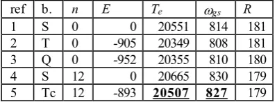
2.2.8 Identification of given chemical species –
individual component assignment problem
Neither FATS nor PARAFAC could provide us with definite answer on chemical composition of samples in question alone. After the data analysis, we are left with a list with rows m, m, (T00,m, gs,m, …) for m {1, 2, …,
f} only. The interpretation to which chemical species m = 1, m = 2, …, m = f components correspond is yet to be done. There are several possibilities for the above mentioned assignment:
a) Literature search for experimental spectra b) Experimental speciation study (cryo-TRLFS
measurement on series of artificial samples (solutions made from pure chemicals as UO3,
Na2CO3, Na2SO4, CaSO4, …))
c) Quantum-chemical modelling (self-made or literature search).
d) By comparison of PARAFAC obtained luminescence-speciation and geochemical model (provided, e.g. by PhreeqC modelling based on existing thermodynamic properties database).
3
Experimentals
3.1 Sample characterization
Samples orginated from a flooded uranium mine prior (S1) and after water treatment (S2) and from seepage water of uranium processing tailings management facilities (TMF’s; S3 – S5, S9).
Samples S5 and S4 have been created by hydrochloric acidification of sample S3 to pH = 6 and 5.5, respectively to investigate acidification driven speciation change.
Table 1 gives total elemental concentrations in mg/l, pH and EH in mV, sample number is written in the
first row. S(VI) stands for sulfate SO42-, C(IV) for
hydrogencarbonates (bicarbonates) HCO3- and carbonates
(CO32-, except for S9 almost all C(IV) is in the form of
HCO3-), N(V) for NO3-.
Table 1: Total elemental conc. (mg/l, adopted from [66]) E \ S 1 2 3 4 5 9 Na 121 122 1350 1550 1580 2520 K 12.8 12.8 27.4
Mg 104 100 301 333 340 61.8 Ca 158 191 292 296 302 86.5 Fe 5.09 0.18 0.28 0.08 Mn 2.17 1.4 0.482
U 1.68 0.02 3.1 3.38 3.53 10.8 Cl 54.3 452 496 908 815 1170 S(VI) 576 546 3620 4030 4100 3150 C(IV) 574 14 657 113 300 2244 N(V) <0.5 <0.5 3.6
pH 7.1 7.4 7.3 5.5 6 9.3 EH 130 450 310 310 310 400
3.2 Measurement
The measurements have been done by HZDR collective [66]. Briefly, samples have been cooled by liquid nitrogen into solid ice-blocks inside plastic cuvette and then placed into cryostat set to (-120±2)°C (Cool gas system TG-KKK produced by KGW). After 15 minutes for temperature equilibration, Time-Resolved Laser-Induced Fluorescence Spectra (TRLFS) has been recorded with pulse energy 1 mJ, excitation wave-length 266 nm and pulse duration 2 ns. Emission wave-length measurement range has been set to 450-650 nm. Minilite Laser System (produced by Continuum) with Spectrograph and ICCD-camera iHR 550 (HORIBA Jobin) has been used. For the spectra recording, software LabSpec has been used [65].
Emission wave-length sampling corresponded to average step of d = 0.463 nm (i.e. d = 18.5 cm-1 for =
1/ = 20000 cm-1). Time series (series of spectra differing
by time interval ti between laser excitation and start of
emission spectra recording) consistend of three types – short („D2“, s = 41 points, dt = 0.05 ms, i.e. t41 = 2.001
ms), long („D3“, s = 51 points, dt = 0.1 ms, i.e. t51 =
5.001 ms), very long („D4“, s = 100 points, dt = 0.101 ms, i.e. t100 = 10 ms). Sample S1 has been measured with
D3 temporal sampling, samples S2, S3, S5 and S9 with D2+D3 sampling, sample S4 with D3+D4 sampling.
For PARAFAC data analysis D3 sampled kinetic series from samples S1-S5 and S9 have been the input.
4
Data analysis of Experimental results
4.1 FATS computationals
The SVD decomposition as described in 2.2.1-2.2.3 has been applied with weighting-preprocessingl [3,5,7,50,51]
such that original measurement data matrix elements Yli
has been transformed onto Y’li normalized data matrix via
l i l i l i Y Y P Q
, (26)
where PlQi represent separable form of variance of Yli, so
Y’li are now closer to case of independent and identicaly
distributed random variables. Since greater variance lies along temporal domain, Pl can be set as Pl = 1 and Qi has,
in software MyExpFit V4 [98] (used for all FATS computations, written in Matlab [99]), general form
i l l i
Q mean Y , (27)
where (0;1). For purely poisson noise, = 0.5, this choice has been applied here. After SVD procedure (4), (5), YU W V T , the subspectra and loadings should be „denormalized“ back according to formulae below,
l j l j l
U U P , (28)
i j i j i
V V Q . (29)
The factor dimension f can be, in general case, determined according to three different diagnostics [3,5,7,50,51]:
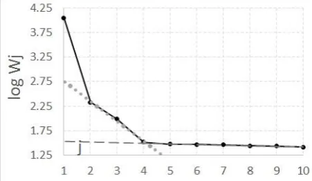
i) SCREE-plot diagnostics [63,64] focus on crossing of linear branches in log Wj = f(j)
plot (Fig. 1). On example for sample S3, f = 3 or f = 4 since the last branch with smallest slope corresponds to noise, but from SCREE-plot alone it is hard to recognize whether still to include j = 4 component or not.
ii) Loadings-based V-diagnostics focus on number of first, signal-like, loadings. For S3 sample, Fig. 2 and Fig. 3 show three signal-like loadings. Since fourth, loadings are much more noise-like (Fig. 4).
iii) Subspectra-based U-diagnostics works as previous, except for subspectra. Fig. 5 presents first three signal-like subspectra, Fig. 6 subspectrum U4’ already noise-like.
While ii) and iii) diagnostics for the chosen example (Sample S3 TRLFS kinetic series analysis) suggest to accept f = 3 components for further analysis, it is better just to conclude that it is possible to statistically distinguish N = 3 independent luminescence active species (according to the geochemical modelling it should be Ca2UO2(CO3)30, CaUO2(CO3)32- and most
probably MgUO2(CO3)32-), but set f = N + 1 = 4.
Because the software based background correction/subtraction [65] is rather approximate, irrespectively to method free parameter choice, FATS for f > 2 provide one individual component with several orders of magnitude larger life-time (and smaller luminescence amount) and bandless continuum-like luminescence spectrum. This component corresponds to background artifact and is ignored in further analysis. Therefore, for N chemical component model, f = N + 1 has to be chosen. By preliminary analysis of randomness of residuals, case N = 1 has been found as insufficient for any sample investigated below, N = 2 as a slight under-fit and N = 4 as a slight over-fit.
Fig. 1. SCREE plot for NmSVD of connected TRLFS kinetic series for sample S3. Wj = Wjj is the j-th singular value, j on horizontal axis. The singular values are plotted as black circles connected by thick lines. Dashed and dotted lines correspond to linear approximation of j = 5 to 10 and j = 2 to 4 regions, respectively.
Fig. 2. NmSVD Loadings (sample S3) of the first two components (j = 1 (black) and j = 2 (gray)).
Fig. 3. NmSVD Loadings (sample S3) of third component (j = 3, still considered as signal).
Fig. 4. NmSVD Loading (Sample S3) of fourth component – very noisy, represent background and noise. Last loading taken into further analysis.
l j l j l
U U P , (28)
i j i j i
V V Q . (29)
The factor dimension f can be, in general case, determined according to three different diagnostics [3,5,7,50,51]:
i) SCREE-plot diagnostics [63,64] focus on crossing of linear branches in log Wj = f(j) plot (Fig. 1). On example for sample S3, f = 3 or f = 4 since the last branch with smallest slope corresponds to noise, but from SCREE-plot alone it is hard to recognize whether still to include j = 4 component or not.
ii) Loadings-based V-diagnostics focus on number of first, signal-like, loadings. For S3 sample, Fig. 2 and Fig. 3 show three signal-like loadings. Since fourth, loadings are much more noise-like (Fig. 4).
iii) Subspectra-based U-diagnostics works as previous, except for subspectra. Fig. 5 presents first three signal-like subspectra, Fig. 6 subspectrum U4’ already noise-like.
While ii) and iii) diagnostics for the chosen example (Sample S3 TRLFS kinetic series analysis) suggest to accept f = 3 components for further analysis, it is better just to conclude that it is possible to statistically distinguish N = 3 independent luminescence active species (according to the geochemical modelling it should be Ca2UO2(CO3)30, CaUO2(CO3)32- and most probably MgUO2(CO3)32-), but set f = N + 1 = 4.
Because the software based background correction/subtraction [65] is rather approximate, irrespectively to method free parameter choice, FATS for f > 2 provide one individual component with several orders of magnitude larger life-time (and smaller luminescence amount) and bandless continuum-like luminescence spectrum. This component corresponds to background artifact and is ignored in further analysis. Therefore, for N chemical component model, f = N + 1 has to be chosen. By preliminary analysis of randomness of residuals, case N = 1 has been found as insufficient for any sample investigated below, N = 2 as a slight under-fit and N = 4 as a slight over-fit.
Fig. 1. SCREE plot for NmSVD of connected TRLFS kinetic series for sample S3. Wj = Wjj is the j-th singular value, j on horizontal axis. The singular values are plotted as black circles connected by thick lines. Dashed and dotted lines correspond to linear approximation of j = 5 to 10 and j = 2 to 4 regions, respectively.
Fig. 2. NmSVD Loadings (sample S3) of the first two components (j = 1 (black) and j = 2 (gray)).
Fig. 3. NmSVD Loadings (sample S3) of third component (j = 3, still considered as signal).
Fig. 4. NmSVD Loading (Sample S3) of fourth component – very noisy, represent background and noise. Last loading taken into further analysis.
Fig. 5. NmSVD subspectra corresponding to the first three components (j {1,2,3}), clearly corresponding to subspace of
signal (in RN, where N = 419 is number of spectral points
selected).
Fig. 6. First, NmSVD subspectrum U’4 corresponding to noise has been added to further analysis for the need to represent background subtraction artifact, but subspectra for j > 4 are omitted from further analysis.
4.2 Sample S1 (mine water)
NmSVD for this sample suggest N = 3 (or 2) and therefore f = 4 (or 3) (Fig. 7). Denormalized f loadings from NmSVD has been fitted to linear combination of f exponential decays, resulting luminescence amounts m [103 ms-1] and life-times m [ms] are presented in Tab. 2.
Fig. 7: NmSVD SCREE-plot and U-diagnostics done by MyExpFit V4 program [98].
FATS f = 3 and f = 4 analysis has been done. Resulting individual component spectra (Fig. 8, Fig. 9) in the former case contained “structure” inside the background component (dotted in Fig. 8) which favoured latter f parameter choice. Please note the peak maxima (e.g. for the highest peak) of the component differs by a tiny portion of 0.86 nm (less than twice of wave-length sampling period!) for f = 3 and 1 nm ( 50 cm-1 in this region) for the two charged complex species for f = 4 as well.
Fig. 8. FATS, f = 3 analysis of sample S1 results for individual component spectra (nm scale).
Fig. 9. FATS, f = 4 analysis of sample S1 results for individual component spectra (nm scale, for better visibility of peak position differences, only three largest peak detail is shown).
Spectroscopic parameters – T00 [103 cm-1] (excitation energy) and gs [cm-1] (ground state vibrational frequency) have been calculated from gaussian fits of FATS f = 4 individual component spectra (Tab. 2, Fig. 10, 11 as an example for m = 1 component).
Fig. 10. m = 1, 1 = 0.87 ms component (assigned to MgUO2(CO3)32-) of f = 4 FATS decomposed according to (19)
Fig. 11.m = 1 component (f = 4), intesity plotted in logarithmic scale to show approximate gaussian character for red-most and blue-most tiny peaks too.
For this sample, an example of R estimation from experimental data is shown in Fig. 12 and Fig. 13, where one and two hot band models, respectively, have been used. In their comparison, two hot band model seems to be more realistic with R = (7.3 ± 1.0) pm
Fig. 12. FATS f = 4, m = 0 (0 = 0.36 ms, assigned to CaUO2(CO3)32-) Franck-Condon fit (23) within „one hot-band“
model. Fitted R = (10.4 ± 1.0) pm. On vertical axis, n’→0 peak area (22) relative to 0’→0 peak is plotted. Horizontal axis represents vibrational number n’.
Fig. 13. FATS f = 4, m = 0 as in previous Fig. 11, but within
„two hot bands“ model. R = (7.3 ± 1.0) pm. The dashed lines
corresponds to R = (R)min ± 0.7 pm, the dotted lines to R =
(R)min ± 1.3 pm, where (R)min is the 2 fit optimum value.
Table 2: FATS f = 4 results for sample S1.
m m m T00,m gs
0 0.36 8.1 20.01 ± 0.01 794 1 0.87 30.1 19.97 ± 0.02 816 2 1.52 4.51 19.92 ± 0.03 807 3 9.52 0.09 n.d. n.d.
4.3 Sample S2 (treated mine water)
Same procedure as for S1 has been repeated, results are presented in Table 3 below (since now, background component is not listed). The uncertainities are (gs) 10cm-1, (m) 0.1 ms and (m) 0.2 ms-1.
Table 3: FATS analysis results, sample S2 (treated mine water)
f m m m T00,m gs
3 0 0.45 2.57 19.98 ± 0.01 804 1 1.15 2.53 19.94 ± 0.02 833 4 0 0.21 1.83 20.07 ± 0.04 798m
1 0.76 2.38 19.97 ± 0.02 810 2 1.26 1.55 19.92 ± 0.03 830
4.4 Sample S3 (TMF seepage water)
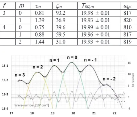
NmSVD and FATS as done for previous samples revealed following parameters (Tab. 4). Due to the higher uranium content, signal:noise ratio has been higher and smoother individual component spectra resulted (Fig. 14). An example of fitting procedure for T00, and gs, determination is presented in Fig. 15, the uncertainities are lower than in S1 by roughly factor of 2.
Table 4: FATS analysis results, sample S3 (TMF seepage water)
f m m m T00,m gs
3 0 0.81 93.2 19.98 ± 0.01 817 1 1.39 36.9 19.93 ± 0.01 820 4 0 0.75 39.6 19.99 ± 0.01 810 1 0.88 59.5 19.96 ± 0.01 817 2 1.44 31.0 19.93 ± 0.01 819
Fig. 14: FATS (f = 4), m = 2 individual component spectrum (later assigned to Ca2UO2(CO3)30) fitted to linear combination
of gaussian profiles. Peak maxima has been fitted as a function of peak number n in follow Fig. 15.
m However after not one but two redmost peaks are excluded
![Table 1: Total elemental conc. (mg/l, adopted from [66])](https://thumb-us.123doks.com/thumbv2/123dok_us/8129871.1354829/7.595.49.292.631.786/table-total-elemental-conc-mg-l-adopted-from.webp)

![Table 12: Excited electronic state properties of [UOCO2(2-3)2(H2O)]2-.](https://thumb-us.123doks.com/thumbv2/123dok_us/8129871.1354829/14.595.54.288.254.426/table-excited-electronic-state-properties-uoco-h-o.webp)