ABSTRACT
AN, MURAT. Clifford Algebraic Structure Study of the Interpolating Spinors and Electromagn-etic Fields between the Instant Form Dynamics and the Light-Front Dynamics with an applicati-on to the Virtual Comptapplicati-on Scattering. (Under the directiapplicati-on of Chueng Ji.)
We study the common general Clifford algebraic structure shared by the Poincar´e ma-trix and the electromagnetic field strength tensor and present the explicit interpolating spinor representations and electromagnetic fields between the instant form dynamics (IFD) and the light-front dynamics (LFD). We also apply our interpolating spinor representations to the anal-ysis of virtual Compton scattering process in an attempt to support the analanal-ysis of the deeply virtual Compton scattering on4He target in Jefferson Lab.
We begin by constructing the generalized interpolating helicity spinors in chiral represen-tation of (J,0)⊕(0, J) Lorentz group between the IFD and the LFD. Our analysis of inter-polating scattering amplitudes shows that the broken symmetry under the longitudinal boost,
P3↔ −P3, is restored only in the LFD.
We derive a direct connection between the polarization vectors in the (1/2,1/2) representa-tion and the spin-1 spinors in the (1,0)⊕(0,1) representation by using the relationship between the gauge fields and the electromagnetic fields and express this connection as a 4×6 transfor-mation matrix between the two representations. Interpolating polarization vectors lead to the interpolating electromagnetic fields in the (1,0)⊕(0,1) representation, which is used to derive the general solution of the Lorentz force equation. We investigate the kinematic and dynamic operator properties of the interpolating electromagnetic field strength tensor for the uniform constant fields and discuss how the number of fields corresponding to the dynamic operators changes between the IFD and the LFD.
As the Clifford algebra (1,3) (Cl1,3) has been a useful tool for the orthochronous Lorentz
transformations, the complex Clifford algebra Cl1,3(C) is used for the derivation of spinors for
the spin-1/2 and spin-1 particles. In addition to the well-known symmetric part of the tensor, composed of the photon polarization vector and its conjugate, we derive the anti-symmetric part of the tensor using the spinor definition ofCl1,3(C).
Clifford Algebraic Structure Study of the Interpolating Spinors and Electromagn- etic Fields between the Instant Form Dynamics and the Light-Front Dynamics with an applicati- on to
the Virtual Compton Scattering
by Murat An
A dissertation submitted to the Graduate Faculty of North Carolina State University
in partial fulfillment of the requirements for the Degree of
Doctor of Philosophy
Physics
Raleigh, North Carolina 2016
APPROVED BY:
Dean Lee John Brown
Ronald Fulp Danesha Seth Carley
Chueng Ji
DEDICATION
BIOGRAPHY
The author was born in a small city Mu˘gla, Turkey. He went to Middle East Technical University to major physics and mathematics in 2001.
ACKNOWLEDGEMENTS
I would like to thank Dr. Chueng Ji for his help, guidance, and patience. I wish to thank Dr. Ben Bakker with our discussions and for his contributions to my projects.
TABLE OF CONTENTS
List of Tables . . . .viii
List of Figures . . . ix
Chapter 1 Introduction . . . 1
1.1 Instant and Light-front Forms . . . 3
1.1.1 Lorentz Transformations . . . 4
1.1.2 Light-front Lorentz Transformations . . . 6
1.2 Interpolating Form . . . 7
1.3 Outline of the Rest of the Dissertation . . . 10
Chapter 2 Interpolating Helicity Spinors and Scattering Amplitudes . . . 12
2.1 Spinors . . . 12
2.1.1 Light-front Boost . . . 16
2.1.2 Light-front Spinors . . . 17
2.2 Interpolating Transformation . . . 18
2.2.1 Interpolating Transformation Operator . . . 21
2.2.2 Finding Interpolating Spinors . . . 23
2.3 Time Ordered Scattering Amplitudes . . . 28
2.4 Annihilation Amplitudes for Fermions . . . 31
2.4.1 High Energy Annihilation Amplitudes . . . 31
2.4.2 Amplitudes without Neglecting Mass Terms . . . 33
2.4.3 Amplitudes in the Interpolating Form . . . 34
2.5 Summary and Conclusions . . . 37
Chapter 3 Interpolating Electromagnetic Field Strength Tensor . . . 39
3.1 Introduction . . . 39
3.2 Electric and Magnetic field Equation of Motion Solutions with Interpolating Quantization . . . 40
3.3 Polarization Vector and Electromagnetic Field Strength . . . 40
3.3.1 Lorentz Force . . . 41
3.3.2 Lorentz Transformation and Electromagnetic Field Tensor . . . 42
3.4 General Solution of Motion in a Uniform Electromagnetic Field . . . 42
3.4.1 Interpolating Form . . . 53
3.5 Summary and Discussion . . . 54
Chapter 4 Clifford Algebra and Spinors. . . 56
4.1 Introduction . . . 56
4.2 Clifford Algebra . . . 57
4.2.1 A Little History About the Clifford Algebra . . . 57
4.2.2 Complex Numbers . . . 58
4.2.3 Quaternions . . . 59
4.2.5 Clifford Algebra (1,3)Cl1,3 . . . 61
4.2.6 Grades . . . 62
4.2.7 Lorentz Transformations . . . 62
4.3 Interpolation Quantization and Spinors with Clifford Algebra . . . 63
4.4 Spinors . . . 64
4.4.1 Anti-symmetry Polarization in Spin-1 Spinors . . . 72
4.5 Interpolating Spinors . . . 74
4.6 Electrodynamics with Clifford Algebra . . . 75
4.7 Summary . . . 76
Chapter 5 Deeply Virtual Compton Scattering and Bethe Heitler Process Update . . . 77
5.1 Introduction . . . 77
5.2 Generalized Hadronic Tensor Structure . . . 78
5.2.1 Comparision of two VCS Tensors and Form Factors . . . 80
5.3 Cross Sections for Virtual Compton Scattering with Angular Dependence . . . . 81
5.4 Hadronic Tensor with CFFs . . . 82
5.5 Kinematics of VCS . . . 83
5.6 Bethe-Heitler Process . . . 83
5.7 Deeply Virtual Compton Scattering (DVCS) . . . 85
5.8 DVCS-Bethe-Heitler Interference Term . . . 87
5.9 Loop Calculations . . . 88
5.9.1 Feynman Rules . . . 88
5.9.2 Passarino-Veltman Integrals . . . 89
5.9.3 Scalar Field with Scalar Loops . . . 91
5.9.4 CFFs with one Loop Calculation . . . 95
5.10 Summary . . . 98
Chapter 6 Conclusion . . . .100
References. . . .102
Appendices . . . .105
Appendix A Appendix for Chapter 1 and Chapter 2 . . . 106
A.1 Table of Commutation Relation of LFD Poincar´e Generators . . . 106
A.2 The spin-1/2 Spinors in IFD and LFD . . . 107
A.3 Derivation of Polarization Vectors . . . 107
A.3.1 Standard Polarization Vectors in IFD . . . 108
A.3.2 Helicity Polarization Vectors in the Interpolating Dynamics . . . 109
A.3.3 Helicity Polarization Vectors in the IFD . . . 110
A.4 (1,0)⊕(0,1) Lorentz Group Spinors of Spin-1 . . . 110
A.5 Generalized (0, J)⊕(J,0) Helicity Spinors for Arbitrary Interpolation Angle for Spin 1 . . . 112
Appendix B Appendix for Chapter 3 . . . 114
B.2 Light-front Dynamics (LFD) Solutions . . . 118
B.3 2D Trajectory of the Charged Particle on theEx and By field . . . 126
B.3.1 E2>B2 Region Motion . . . 126
B.3.2 E2=B2 Region Motion . . . 132
B.3.3 E2<B2 Region Motion . . . 132
Appendix C Appendix for Chapter 4 . . . 142
C.1 Lorentz Force Equation with Quaternions . . . 142
C.2 4×6 Matrix and Spinors . . . 143
C.3 (1,0)⊕(0,1) Spinors and new Dirac Gamma Matrices . . . 147
C.4 Electric and Magnetic Field Function in Momentum Space . . . 148
Appendix D Appendix for Chapter 5 . . . 149
D.1 Kinematics of DVCS and BH Process with Angular Dependence . . . 149
D.2 Bethe-Heitler Lepton Tensor . . . 151
LIST OF TABLES
Table 1.1 Poincar´e Algebra for any interpolation angle. The commutation relation reads [element in the first column, element in the first row] = element at the intersection of the corresponding row and column. . . 9 Table 1.2 Kinematic and dynamic generators for different interpolation angles . . . . 10 Table A.1 Poincar´e Algebra for LFD. The commutation relation reads [element in
the first column, element in the first row] = element at the intersection of the corresponding row and column. . . 106 Table A.2 Spinors at light-front limit (δ →π/4) . . . 107 Table A.3 Spinors at instant form limit (δ →0). HereN =
√ M √
2|P⃗|(P0+|P|)(P3+|P|) and
LIST OF FIGURES
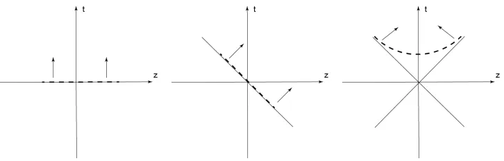
Figure 1.1 Three forms of dynamics: (a) the instant form, (b) the light-front, and (c) the point form. The dashed lines are the quantization surfaces and the arrows are their time evolution direction. . . 1 Figure 2.1 An illustration of the relations between different conventions and names
we use in this dissertation. The red letters C and S stand for chiral and standard representations respectively. The blue letters H and D stand for helicity spinor and Dirac spinor respectively. The solid black arrow points from the instant form to the light front form, and the interpolation angle
δ goes from 0 toπ/4. Both the helicity and Dirac spinors can be generated for arbitrary interpolation angle. The dashed purple arrow indicates the Melosh transformation, which relates the instant Dirac spinor to the light-front helicity spinor. . . 13 Figure 2.2 Time ordered amplitudes in IFD. . . 28 Figure 2.3 Interpolating amplitudes. . . 30 Figure 2.4 e−e+ → µ−µ+ annihilation at angle θ, and its corresponding Feynman
diagram at the lowest tree level. . . 31 Figure 2.5 (Color online) fermion annihilation amplitudes (with the factor −e2/q2
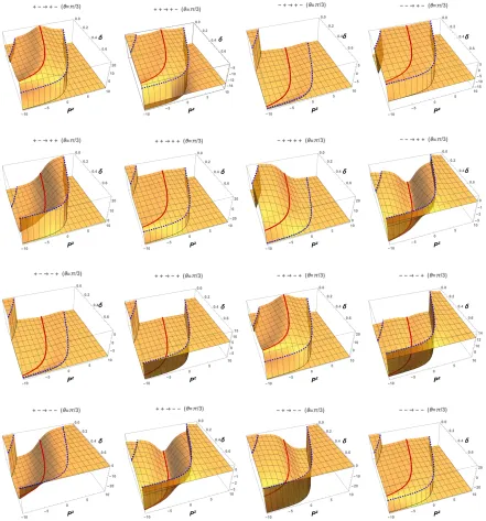
dropped) for 16 different spin configurations with the center of mass en-ergyM = 4 GeV and the annihilation angleθ=π/3. The two blue dashed lines are the boundary lines across which the values of helicity amplitudes suddenly change and the red solid line is the universal J-curve mentioned. 35 Figure 2.6 (Color online) fermion annihilation probabilities (with the factor −e2/q2
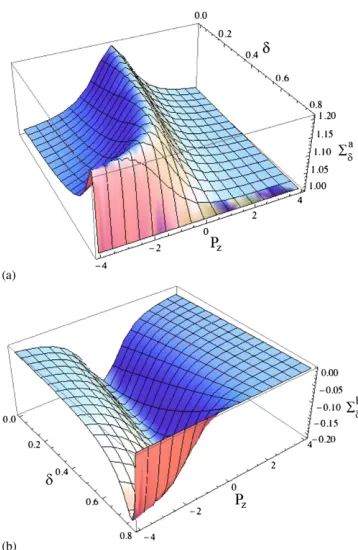
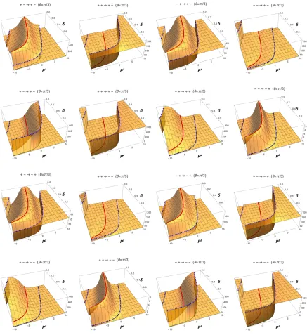
dropped) for 16 different spin configurations with the center of mass en-ergyM = 4 GeV and the annihilation angleθ=π/3. The two blue dashed lines are the boundary lines across which the values of helicity amplitudes suddenly change and the red solid line is the universal J-curve mentioned. 36 Figure 2.7 The total annihilation probability (with the factor (e2/q2)2 dropped) as a
sum of all spin contributions (helicity probabilities plotted in Figure 2.6) for the lowest tree diagram shown in Figure 2.4. . . 37 Figure 3.1 u+ˆ(τ) plot when E
x = Bytanδ and Ey = Bxtanδ and u+ˆ becomes invariant at δ ={0, .46365, π/4} respectively. The blue graph represents
u+ˆ(τ) and the orange one is where it is invariant. Here Bx = 1T, By = −2T, Bz = 3T, the initial velocity vz(0) = 0.2c, and m is taken as unit mass 1 for illustration. . . 54 Figure 3.2 log
(
u+ˆ(τ) )
plot when there is Ez and u+ˆ becomes invariant at δ =
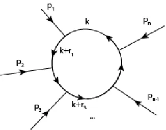
Figure 5.1 Handbag diagram for s-channel virtual Compton scattering.k is the mo-mentum of a quark that hit by a virtual photon and the final photon q′
is a real photon. . . 78
Figure 5.2 sQED tree-level Feynman amplitudes: Seagull, s-channel, and u-channel. . 79
Figure 5.3 Compton scatterig between electron and Hadron have two parts: DVCS and Bethe-Heitler process . . . 82
Figure 5.4 Compton scattering of real photons . . . 84
Figure 5.5 ri related with external momenta. . . 89
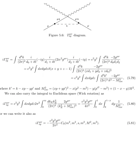
Figure 5.6 Tsgµν diagram. . . 91
Figure 5.7 Wstµν diagram. . . 92
Figure 5.8 Ustµν diagram. . . 92
Figure 5.9 Vstµν diagram. . . 93
Figure 5.10 Tstµν diagram. . . 94
Figure 5.11 Tutµν diagram. . . 94
Figure B.1 First plot is|E|>|B|and second plot is|E|<|B|.BxandBy are pulling down in the -z direction opposite have force in the +z direction by Ez. Here Bx = By = 0.1T, Ez/c = {0.1,0.05}T , Bz = {0.05,0.1}T, and vz0 = 0.5c . . . 124
Figure B.2 Trajectory of the charged particle when there is no magnetic field (Ex/c= 0.001T andBy = 0) respectively the blue trajectory is whenvz(0) = 0.1c, the red trajectory is when vz(0) = 0.5c, and the green trajectory is when vz(0) = 0.9c . . . 127
Figure B.3 Trajectory of the charged particle when Ex/By > c (Ex/c = 0.01T and By = 0.005T) here is the blue trajectory is when vz(0) = 0.1c, the red one is when vz(0) = 0.5c, and the green one is whenvz(0) = 0.9c. . . 128
Figure B.4 Trajectory of the charged particle whenEx/By > candEx ∼By(Ex/c= 0.01T and By = 0.009T) here is the blue trajectory is when v0z = 0.1c, the red one is when vz(0) = 0.5c, and the green one is whenvz(0) = 0.9c. . 129
Figure B.5 Trajectory of the charged particle whenEx/By >1 for different magnetic fields (Ex/c = 0.01T and vz0 = 0.5c) here is the blue trajectory is when By = 0.001T, the orange one is whenBy = 0.005T, and the green one is when By = 0.009T, the trajectory is getting closer to negative x-axis as magnetic field increase. . . 129
Figure B.6 Trajectory of the charged particle whenEx/By = √ 2c(Ex/c= 0.141421356T and By = 0.1T) for 1/60th of second interval and the blue trajectory is when vz(0) = 0.1c, the red one is whenvz(0) = 0.5c, and the green one is when vz(0) = 0.9c . . . 130
Figure B.8 Initial time trajectories for less than 5 second motions with their short time approaches which dominated by initial velocity vz(0) in case of
Ex > By (Ex/c = 0.005T and By = 0.001T). Here there are tree cases:
vz(0) = 0.1c case, real trajectory (blue color) and short time approxima-tion (dashed cyan color) ,vz(0) = 0.5c case, real trajectory (red color) and short time approximation (dashed orange color), vz(0) = 0.9c case, real trajectory (green color) and short time approximation (dashed brown color). . . 136 Figure B.9 The trajectory change between the initial approached (orange dashed)
and the long time approached (blue dashed) motions for Ex/c= 0.005T and By = 0.002T withvz(0) = 0.5c . . . 137 Figure B.10 Trajectory of the charged particle whenEx/c=By = 0.01T and the blue
trajectory is when vz(0) = 0.1c, the red trajectory is when vz(0) = 0.5c, and the green trajectory is when vz(0) = 0.9c. . . 137 Figure B.11 Trajectory of the positive charge when By > Ex (Ex/c = 0.25T and
By = 0.5T). The blue trajectory is when vz(0) = 0.1c, the red one is when vz(0) = 0.5c, and the green one is when vz(0) = 0.9c . . . 138 Figure B.12 Trajectory of the charged particle when Ex/By < 1 (Ex/c = 0.1T and
By = 0.373205T) and here the red trajecory whenv0z = 0.5cis the turning point of helical waves, when v0z = 0.9c the green trajectory has helical waves, and the blue trajectory has regular waves when vz0= 0.1c . . . 139 Figure B.13 The trajectory of charged particle whenEx= 0 andBy = 0.5T >0, here
respectively the blue trajectory is when vz(0) = 0.1c, the red trajectory is when vz(0) = 0.5c, and the green trajectory is when vz(0) = 0.9c. . . 140 Figure B.14 Initial time trajectories for less than 1 second motions with their short
time approaches which dominated by initial velocity vz(0) in case of
By > Ex(Ex/c= 0.001T andBy = 0.005T). Three cases are :vz(0) = 0.1c case, real trajectory (blue color) and short time approximation (dashed cyan color),vz(0) = 0.5c case, real trajectory (red color) and short time approximation (dashed orange color), and .vz(0) = 0.9ccase, real trajec-tory (green color) and short time approximation (dashed brown color). . . 141 Figure D.1 Bethe Heitler process of incoming photon beam making Compton
Chapter 1
Introduction
Dirac proposed three forms of relativistic Hamiltonian dynamics in 1949 [1], instant form dy-namics (IFD) (x0 = 0), light-front dynamics (LFD) (x+= (x0+x3)/√2 = 0) and point form
(x2 =a2 > 0, x0 > 0). Although the point form’s exploration is recent [2], the instant form ( the equal time t) and the light-front (the equal timeτ =t+z/c) have been the most popular choices.
Figure 1.1: Three forms of dynamics: (a) the instant form, (b) the light-front, and (c) the point form. The dashed lines are the quantization surfaces and the arrows are their time evolution direction.
Secondly, the dispersion relation of the energy-momentum in instant form is given by
k0 =√k2+m2, (1.1)
wherek0 is energy and kis momentum vector.
In the light-front, the dispersion relation is given by
k−k+=|k⊥|2+m2, (1.2) wherek−= (k0−k3)/√2 andk+= (k0+k3)/√2. Though Eq. 1.1 shows an irrational relation between energy and momentum, Eq. 1.2 yields a rational relation. It correlates the light-front energyk− andk+and makes relations simpler. In the LFD when the light-front time is positive so is the momentum (k+). This property of the LFD also leads to preventing the random creation of pair particles unlessk+= 0.
There is no spontaneous creation in the light front vacuum. A constituent-type model in which all partons in a hadronic state are connected with hadrons instead of vacuum fluctuations can be obtained [3].
The interpolation between the IFD and the LFD provides a complete picture of the land-scape between the two and clarifies the issue, if any, in linking them to each other. The same method of interpolating hypersurfaces has been used by Hornbostel [4] to analyze various as-pects of field theories, including the issue of a nontrivial vacuum. The same kind of application to study the axial anomaly in the Schwinger model has also been presented [5], and other related works [6],[7], [8], [9],[10] can also be found in the literature.
LFD has the maximum number of kinematic generators compared to other forms of dy-namics. There are seven kinematic generators which leave light-front time (x+) invariant [11].
The study of the Poincar´e algebra for any arbitrary interpolation angle started with [12] and recently provided the physical meaning of the kinematic vs. dynamic operators by introduc-ing the interpolatintroduc-ing time-ordered scatterintroduc-ing amplitudes [13]. In particular, we demonstrated that the longitudinal boost invariance of each individual x+ˆ-ordered scattering amplitudes is realized only at δ =π/4 and the disappearance of the connected contributions to the current arising from the vacuum occurs independent of the reference frame only when the interpolation angle is taken to yield the LFD. This affirms the well-known saga of the longitudinal boostK3
which maximizes the number of kinematic (i.e. interaction independent) generators in LFD as seven out of ten Poincar´e generators. Dramatic character change of K3 from “dynamic” for 0≤δ≤π/4 to “kinematic” inδ=π/4 greatly benefits the use of LFD for the study of hadron physics.
infinite momentum frame (IMF). It thus resolves the confusion in the prevailing notion of equivalence between the LFD and the IMF. For the study of hadron physics in QCD, the built-in boost built-invariance together with the simpler vacuum property built-in LFD is certabuilt-inly an appealbuilt-ing feature as it may save substantial computational efforts in getting QCD solutions that respect the full Poincar´e symmetries.
Although we want ultimately to obtain a general formulation for the QCD using the in-terpolation between the IFD and the LFD, we start from the simpler theory to discuss first the bare-bone structure that will persist even in the more complicated theories. Subsequent to our study of the simple scalar field theory [13] involving just the fundamental degrees of freedom such as the momenta of particles in scattering processes, we considered very recently interpolating the electromagnetic gauge degree of freedom between the IFD and the LFD and found that the light-front gauge in the LFD is naturally linked to the Coulomb gauge in the IFD through the interpolation angle [14]. We also extended our interpolation of the scattering amplitude presented in the simple scalar field theory [13] to the case of the electromagnetic gauge field theory but still with the scalar fermion fields known as the sQED theory [14] and analyzed the lowest scattering processes in sQED such as the analogues of the well-known QED processe+e−→µ+µ−.
1.1
Instant and Light-front Forms
The instant form quantization and the light-front quantization are the most popular choices among the three types of quantizations.
On light-front quantization, the equal time is defined as on the light-cone.
x+ = √1
2(t+z), (1.3)
x1 = x, (1.4)
x2 = y, (1.5)
x− = √1
2(t−z). (1.6)
The change of equal time brings a corresponding spatial coordinate change alsox−. Thex and
y coordinates remain unchanged. Here, the speed of lightc is taken as 1.
x+ x1 x2 x− = 1 √
2 0 0
1
√
2
0 1 0 0
0 0 1 0
1
√
2 0 0 −
1 √ 2 x0 x1 x2 x3
. (1.7)
The metric tensor on light-front is
gµν =
0 0 0 1
0 −1 0 0 0 0 −1 0
1 0 0 0
. (1.8)
1.1.1 Lorentz Transformations
Lorentz transformation replaces the Galilean transformation with the additional dimension of Einstein’s special theory of relativity. A Lorentz transformation is a four dimensional transfor-mation and is usually represented byΛµν as
xµ′ =Λµνxν, (1.9)
However we use the inhomogeneous Lorentz transformation or Poincar´e transformation which is described as
xµ′=Λµνxν+aµ. (1.10) Here aµ is a constant four vector. Λ must satisfy
gαβΛαµΛβν =gµν. (1.11) Weinberg [15] and some other authors refer to Poincar´e transformations as Lorentz transfor-mations in their work. Poincar´e transformations (inhomogeneous Lorentz transformations) can be homogeneous Lorentz transformations when aµ= 0 in Eq. 1.10.
The Lorentz transformation can be written as an infinitesimal transformation up to the second order as
Λµν =δνµ+δϕµν (1.12)
gαβ(δαµ+δϕαµ)(δβν +δϕβν) = gµν
gµν+δϕµν+δϕνµ+O(ϕ2) = gµν. (1.13) The Lorentz condition yields an anti-symmetric tensor
ϕµν =−ϕνµ. (1.14)
An infinitesimal Lorentz transformation with aµ =ϵµ in the Hilbert space can be written as
U(1 +ϕ, ϵ) = 1−1 2iϕ
µνM
µν+iϵµPµ+... (1.15) Here Mµν is an anti-symmetric Lorentz transformation which describes rotation and boost i.e. where
Mµν = {
Mij =ϵijkJk
Mi0 =−Ki
(i, j, k = 1,2,3).
Mµν has a total of 6 components, and with Pµ, an inhomogenous Lorentz transformation has 10 generators. These generators construct a Lie algebra such as
[Mµν, Mρδ] = i(gνρJµδ−gµρJρδ+gµδJνρ−gνδJµρ), (1.16)
[Pµ, Pν] = 0, (1.17)
[Pµ, Mρδ] = i(gµρPδ−gµδPρ). (1.18) We can writeMµν as a matrix form and call it a Poincar´e matrix
Mµν =
0 K1 K2 K3
−K1 0 J3 −J2
−K2 −J3 0 J1
−K3 J2 −J1 0
. (1.19)
There are ten Poincar´e generators and these generators are separated as kinematic and dy-namic generators as shown in Table 1.2 , where kinematic generators do not alter the equal time, on the initial surface. Thus the Hamiltonian becomes invariant in such kinematic operators. As well, [J3, P0] = 0 and invariance is broken under dynamic generators [K3, P0] =iP3 .
The mapping from Lie algebra to Lie group may be expressed as
where the mapping is from the homogenenous Lorentz algebra (Poincar´e algebra) to the group of Lorentz transformation inR1,3 .
By using a matrix exponential, the Lorentz transformation for boost and rotation groups can be written as
Λ(ϕ,θ) =eK.ϕ+J.θ. (1.21) Generators of the Lorentz transformations corresponds to important physical symmetries. The physical symmetry of rotation transformation J corresponds to angular momentum and the physical symmetry of the boost transformation K corresponds to motion in space-time. These transformation generators can be expressed in matrix form as
K1 =
0 1 0 0 1 0 0 0 0 0 0 0 0 0 0 0
, K
2 =
0 0 1 0 0 0 0 0 1 0 0 0 0 0 0 0
, K
3 =
0 0 0 1 0 0 0 0 0 0 0 0 1 0 0 0
, (1.22)
and
J1=
0 0 0 0 0 0 0 0 0 0 0 −1 0 0 1 0
, J
2 =
0 0 0 0 0 0 0 1 0 0 0 0 0 −1 0 0
, J
3 =
0 0 0 0 0 0 −1 0 0 1 0 0 0 0 0 0
. (1.23)
The commutation relations of these matrices in general constructs three cyclic relations as [Ji, Jj] = iϵijkJk, (1.24) [Ki, Kj] = −iϵijkJk, (1.25) [Ji, Kj] = iϵijkKk, (1.26)
1.1.2 Light-front Lorentz Transformations
The four momentum in light-front form is the same as the coordinate changes: P+ = P− = (P0+P3)/√2,P−=P+= (P0−P3)/√2, andP+ =P− is the light-front energy.
Eq. 1.7 as
MLFµν = 1 √
2 0 0
1
√
2
0 1 0 0
0 0 1 0
1
√
2 0 0 −
1 √ 2
0 K1 K2 K3
−K1 0 J3 −J2
−K2 −J3 0 J1
−K3 J2 −J1 0 1 √
2 0 0
1
√
2
0 1 0 0
0 0 1 0
1
√
2 0 0 −
1 √ 2 =
0 E1 E2 −K3
−E1 0 J3 −F1
−E2 −J3 0 −F2 K3 F1 F2 0
, (1.27)
where the light-front generators are expressed as
E1 = √1 2(K
1+J2), (1.28)
E2 = √1 2(K
2−J1), (1.29)
F1 = √1 2(K
1−J2), (1.30)
F2 = √1 2(K
2+J1). (1.31)
Among these ten Poincar´e generators there are only three dynamic generators as shown in Table 1.2. Along with E1 and E2, K3 also becomes a kinematic generator in LFD since [P+, K3] = iP+. Therefore the initial surface x+= 0 becomes invariant under longitudinal boost.
1.2
Interpolating Form
The interpolating quantization where the equal time is defined between the instant timet and the light-front timeτ = (t+z)/√2 by an interpolating angleδsuch thatx+ˆ =tcosδ+zsinδ. In
general we set a space-time coordinate transformation between IFD and LFD by interpolating angle xµˆ =Rµˆνxν, i.e.
x+ˆ xˆ1 xˆ2 x−ˆ
=
cosδ 0 0 sinδ
0 1 0 0
0 0 1 0
sinδ 0 0 −cosδ
x0 x1 x2 x3
where the interpolation angle is 0≤δ ≤π/4. The δ → π/4 limit gives us the light-front form and we recover the instant form at δ→0 limit. The matrix form of Rµˆν is
Rµˆ
ν =
cosδ 0 0 sinδ
0 1 0 0
0 0 1 0
sinδ 0 0 −cosδ
. (1.33)
The metric can be written as
gµˆˆν =RµˆαgαβRνˆα=
C 0 0 S 0 −1 0 0 0 0 −1 0 S 0 0 −C
, (1.34)
whereC refers to cos(2δ), Srefers to sin(2δ), and the inverse one is
Rµνˆ =gµˆαRˆ αˆν =
cosδ 0 0 −sinδ
0 −1 0 0
0 0 −1 0
sinδ 0 0 cosδ
. (1.35)
The energy-momentum transformation will be the same as the coordinate transformation, as we have seen in the light-front case.
P+ˆ = P0cosδ+P3sinδ, (1.36)
Pˆ1 = P1, (1.37)
Pˆ2 = P2, (1.38)
P−ˆ = P0sinδ−P3cosδ. (1.39)
Interpolating Poincar´e Matrix
The Lorentz transformation generators given in the Poincar´e matrix can be written in interpo-lating dynamics similar to Eq. 1.27 as
Mµˆˆν =RµˆαMαβRˆνβ =
0 Eˆ1 Eˆ2 −K3
−Eˆ1 0 J3 −Fˆ1
−Eˆ2 −J3 0 −Fˆ2 K3 Fˆ1 Fˆ2 0
and
Mµˆνˆ=gµˆαˆMαˆ ˆ
βg
ˆ
νβˆ=
0 Dˆ1 Dˆ2 K3
−Dˆ1
0 J3 −Kˆ1
−Dˆ2 −J3 0 −Kˆ2
−K3 Kˆ1 Kˆ2 0
, (1.41)
where
Eˆ1 = K1cosδ+J2sinδ, Dˆ1 =−K1cosδ+J2sinδ, Eˆ2 = K2cosδ−J1sinδ, Dˆ2 =−K2cosδ−J1sinδ, Fˆ1 = K1sinδ−J2cosδ, Kˆ1 =−K1sinδ−J2cosδ,
Fˆ2 = K2sinδ+J1cosδ, Kˆ2 =−K2sinδ+J1cosδ. (1.42) The Poincar´e algebra is constructed by these generators and their commutation relations are given in Table 1.1. As we mentioned before there is one more kinematic generator in LFD. Since only dynamic generators alter the time component, K3 is not a dynamic generator in LFD forx+. Between 0≤δ < π/4 K3 is a dynamic generator forx+ˆ and at δ=π/4, it is not
a dynamic generator.
Table 1.1: Poincar´e Algebra for any interpolation angle. The commutation relation reads [element in the first column, element in the first row] = element at the intersection of the corresponding row and column.
P
+ˆP1
P2
P
−ˆD
1D
2K
3K
1K
2J
3P
+ˆ0
0
0
0
-
i
C
P
1-
i
C
P
2iP
ˆ
−
0
0
0
P1
0
0
0
0
iP
+ˆ0
0
iP
−ˆ0
-
iP2
P2
0
0
0
0
0
iP
+ˆ0
0
iP
−ˆiP1
P
−ˆ0
0
0
0
0
0
iP
+ˆ-
i
S
P
1-
i
S
P
20
D
1i
C
P
1-
iP
ˆ+
0
0
0
iK
3
iF
1-
ij
3S
-
iJ
3C
-
i
D
2D
2i
C
P
20
-
iP
ˆ+
0
iJ
3C
0
iF
2iJ
3S
iK
3i
D
1K
3iP
−ˆ0
0
-
iP
+ˆ-
iF
1-
iF
20
iE
1iE
20
K
10
-
iP
ˆ−
0
i
S
P
1-
iK
3-
iJ
3S
-
iE
10
iJ
3C
-
i
K
2K
20
0
-
iP
ˆ
−
i
S
P
2iJ
3S
-
iK
3-
iE
2-
iJ
3C
0
i
K
1J
30
iP
2-
iP
10
i
D
2-
i
D
10
i
K
2-
i
K
10
Among the covariant Poincar´e generators for any interpolation angle, Kˆ1,Kˆ2, J3, P1, P2, P−ˆ
Table 1.2: Kinematic and dynamic generators for different interpolation angles
Angle Kinematic Dynamic
δ= 0 K1=−J2,K2 =J1, J3, P1, P2, P3 D1=−K1,D2=−K2, K3, P0
0≤δ < π/4 K1,K2, J3, P1, P2, P−ˆ D1,D2, K3, P+ˆ δ=π/4 K1=−E1,K2 =−E2, J3, K3, P1, P2, P+ D1=−F1,D2=−F2, P−
dynamic generators depending on the interpolation angle are presented in Table 1.2.
The subset of the Poincar´e group that doesn’t alter the time evolution parameter x+ˆ is called the stability group. As we can see, in LFD we have the greatest number of kinematic operators, and therefore the largest stability group. Since kinematic transformations don’t alter
x+ˆ, individual time-ordered amplitudes must be invariant under kinematic transformations.
1.3
Outline of the Rest of the Dissertation
As we have introduced interpolating form dynamics between IFD and LFD and the Lorentz transformations in this chapter, Chapter 1, we continue with the spinor representation in in-terpolating form in Chapter 2. We discuss the inin-terpolating transformation operator with the connection of the light-front boost to the Jacob-Wick transformation operator and derive the interpolating spinors in helicity spinor form in chiral representation using the interpolating transformation operator between IFD and LFD. We then find amplitudes of an annihilation and creation scattering amplitude analogous to the electron-muon annihilation in helicity spinors. We observe that at the light-front limit, the amplitudes become frame independent and discuss the reasons behind this phenomena.
In chapter 3, we investigate the interpolating form of the Lorentz force equation for a charged particle under a constant uniform electromagnetic field as continuation of gauge field interpolation work presented in [14]. We discuss the connection between the gauge fields and the electromagnetic fields, i.e. between the four-component polarization vector representation and the six-component spin-1 spinor representation. With the analogy between the electromagnetic field tensor for constant uniform fields and the Poincar´e matrix, we discuss the kinematic and dynamic characteristics in electromagnetism. Similar to the Poincare matrix, the number of dynamic generators gets reduced in the LFD.
spin-1 spinors by using the same transformation. Additionally, the connection of 4 component polarization vectors and 6 component spin-1 spinors is obtained through this algebra and this helps us to the complete polarization tensor’s anti-symmetric part by the relation between these two different spin-1 spinor representations.
As an application of this development of spin-1 spinor representation, we investigate the general structure of hadronic tensor for deeply virtual Compton scattering in Chapter 5. We discuss the simple case where the target is scalar case and get the most general form. The amplitudes of deeply virtual Compton scattering with Bethe-Heitler process are studied as well. One loop calculation is discussed for a scalar particle exchange with the outgoing real photon in terms of Passarino-Veltman functions.
Chapter 2
Interpolating Helicity Spinors and
Scattering Amplitudes
This chapter is about the spinor of interpolating form between instant form and light-front form. We investigate fermion fields in terms of spinors and scattering amplitudes.
To study the properties of a spinor in general, we need to understand that a spinor for a particle is characterized by two pieces of information: the momentum of the particle, and the spin orientation. The helicity spinor defined in the IFD has the spin of the particle either aligned or anti-aligned with its momentum direction. As shown in Figure 2.1, there are two kinds of spinors in terms of spin orientation: Dirac spinor where the spin is in z-direction in the rest frame and helicity spinor where the spin direction is along with the momentum direction. There are two representations of spinor in terms of handedness of particles: Standard representation where the spinor is a combination of right-handed and left-handed spinors as shown in Eq. 2.2 and chiral or Weyl representation where right-handed and left-handed spinors are decoupled. We show first the construction of spinors in IFD and discuss the construction of LFD in chiral representation and compare it with the standard representation. Then we discuss the interpolating spinors. Furthermore, we show an example of amplitudes. We discuss amplitudes of scalar particle spinors and the scattering of fermions using interpolating spinors that we obtained. We discuss the effect of frame dependence on helicity. We investigate the instant front limit (δ → 0) and the light-front limit (δ → π/4) and how spin orientation changes between them.
2.1
Spinors
by
S=S†= √1 2
(
I2 I2 I2 −I2
)
, (2.1)
whereI2 is 2×2 identity matrix. The spinors are related as
ψSR = 1 √ 2
(
ϕR+ϕL
ϕR−ϕL )
= √1 2
(
I2 I2 I2 −I2
) (
ϕR
ϕL )
=SψCR, (2.2)
and the Dirac matrices transform as
γSRµ =SγCRµ S†. (2.3)
There are six generators of the Lorentz group: three boost K and three rotation J gen-erators. We can decouple them in order to construct two SU(2) groups since SO(1,3) ∼
T
D=e
-iη.KT
JW=e
-iθ.Je
-iβ KT T
3 3
SU(2) × SU(2)
SO(1,3)
LFD IFD
SU(2)⊗SU(2) as
A = 1
2(J +iK), (2.4)
B = 1
2(J −iK), (2.5)
and their commutation relations become [
Ai, Aj ]
= iϵijkAk, (2.6)
[
Bi, Bj ]
= iϵijkBk, (2.7)
[
Ai, Bj ]
= 0, (2.8)
fori, j, k = 1,2,3.
We can describe boost and rotation generators inSU(2) as
JR = 1
2σ, KR=
i
2σ, (2.9)
JL = 1
2σ, KL=−
i
2σ, (2.10)
as right-handed and left-handed systems, it is also called type I (0,1/2) and type II (1/2,0) systems. We can combine them together inSU(2)×SU(2) and write them down together as
K = i 2
( σ 0
0 −σ )
, (2.11)
J = 1 2
( σ 0
0 σ )
. (2.12)
We observe that A andB components are formed in matrix representation and they are
A= 1 2
( σ 0
0 0 )
, B= 1 2
( 0 0 0 σ
)
. (2.13)
We can represent Aand B or right-handed or left-handed operators as (J,0)⊕(0, J) in chiral representaion of the Lorentz group.
down for each case at rest as
ψ(x) = u(0)eimt, positive energy, (2.14)
ψ(x) = v(0)e−imt, negative energy. (2.15) With spin conditions the spinors at rest are
u(1)(0) = √ m 0 √ m 0 , u
(2)(0) =
0 √ m 0 √ m , v
(1)(0) =
√ m 0 −√m
0 , v
(2)(0) =
0 √ m 0 −√m
. (2.16)
In chiral representation that is spinor seperated as right-handed and left-handed as ψCR = (
ϕR
ϕL )
.
Since the spinors are decoupled in chiral representation, we use the chiral representation for spinor constructions. In order to carry spinors into the moving frame in terms of Dirac spinors, we use Eq. 2.11 to describe an arbitrary boost to any direction by the rapidityη
(
ϕ′R ϕ′L
) =
(
e12σ.η 0 0 e−12σ.η
) (
ϕR
ϕL )
. (2.17)
The momentum in the moving frame can be written in terms of the boost angles as
cosh(η/2) = (
p0+m
2m
)1/2
, (2.18)
sinh(η/2) = (
p0−m
2m
)1/2
, (2.19)
tanh(η/2) = |p|
p0+m, (2.20)
whereη =√η12+η22+η32. We can write down each individual momentum as
p0 = cosh(η), (2.21)
p1 = η1
η sinh(η), (2.22)
p2 = η2
η sinh(η), (2.23)
p3 = η3
then the spinors in the momentum frame are obtained from the rest spinors that are given by Eq. 2.16 by using e12σ.η = cosh(η/2) + σ
iη i
η sinh(η/2) as follows:
u(1)(p) = 1 2√2
p0+m+p3
√ 2pR p0+m−p3
−√2pR
, u
(2)(p) = 1
2√2 √ 2pL p0+m−p3
−√2pL
p0+m+p3
, (2.25)
v(1)= 1 2√2
p0+m+p3
√ 2pR
−p0−m+p3
√ 2pR
, v
(2)= 1
2√2 √ 2pL p0+m−p3
√ 2pL p0+m+p3
. (2.26)
wherepR= (p1+ip2)/√2 andpL= (p1−ip2)/√2.
2.1.1 Light-front Boost
There are two types of transformation operators which bring the rest frame spinor to the moving frame. The first one is a pure boost in any direction
T =e−iβ.K. (2.27)
The second one is the transformation operator described by Jacob and Wick in [17] and given by
TJ W =e−iθ
⊥.J⊥
e−iβ3K3. (2.28)
This transformation type describes a canonical boost in z-directon first, then rotations to the direction of the momentum. The rotation part enables the spin direction to align with the momentum direction. The initial particle spin direction is in the z-direction.
The light-front transformation operator is given by [18] as
TLF =e−i(β1E
1+β2E2)
e−iβ3K3. (2.29)
The momentum transformation can be obtained by the light-front transformation operator is given by Eq. 2.29 and by using commutation relations in Appendix A.1.
TLF−1P+TLF = eβ3P+, (2.30)
TLF−1P⊥TLF = P⊥+β⊥eβ3P+, (2.31)
We write the momentum of moving particles from the rest frameP0µ= (m,0,0,0) transformed as
P+ = eβ3m, (2.33)
P⊥ = eβ3mβ⊥, (2.34)
P− = e−β3m+eβ3m|β⊥|2. (2.35)
2.1.2 Light-front Spinors
In addition to the Dirac spinors, which can be in standard or chiral (Weyl) representation, we also have helicity spinors. The difference between the Dirac and helicity spinors is how to define momentum direction according to the spin direction. In Dirac spinor, the spin is in the z-direction (positive or negative) in the initial state and momentum is in an arbitrary direction. However, the helicity spinor momentum is defined along with the direction of the spin as we stated in Section 2.1.1 by applying the transformation, which is given by (2.28) by Jacob and Wick [17]. Ahluwalia and Sawicki [19] applied the light-front boost which is given by Eq. 2.29 for finding light-front spinors. In this definition, the spinors at rest are defined the same as the Dirac spinors in chiral representation as in Eq. 2.16. Then the transformation operator, which is given by Eq. 2.28, applies to these spinors to convert it to the moving frame and the light-front helicity operator is given by Eq. 2.29 and used as
ψLF =TLFψCR(0). (2.36)
First, we define TLF in (1/2,0)⊕(0,1/2) Lorentz group. We need to find right-handed and left-handed parts as
TLF = (
TR LF 0 0 TLFL
)
. (2.37)
Then, we use the Eq. 2.9 and Eq. 2.10 notations to find TLF transformation (β1E1+β2E2)R =
1 √
2(β1(iσ
1+σ2) +β
2(iσ2−σ1)), (β3K3)R=iβ3σ3 (2.38)
(β1E1+β2E2)L =
1 √
2(β1(−iσ
1+σ2) +β
By using Eq. 2.33-Eq. 2.35, we get
u(1)CR(p) = √√1 2p+
√ 2p+ pR m 0 , u
(2)
CR(p) = 1 √√
2p+
0 m
−pL
√ 2p+
, (2.40)
v(1)CR(p) = √√1 2p+
√ 2p+ pR −m 0 , v
(2)
CR(p) = 1 √√
2p+
0 m pL
−√2p+
. (2.41)
Converting them in standard representation by S transformation is given by Eq. 2.1, then the spinors are
u(1)SR(p) = √ 1 2√2p+
√
2p++m pR
√
2p+−m pR , u
(2)
SR(p) = 1 √
2√2p+
−pL
√
2p++m pL
−√2p++m
, (2.42)
v(1)SR(p) = √ 1 2√2p+
√
2p+−m pR
√
2p++m pR , v
(2)
SR(p) = 1 √
2√2p+
pL
−√2p++m
−pL
√
2p++m
. (2.43)
2.2
Interpolating Transformation
The interpolating transformation operator is defined to be consistent with the light front boost is given by Eq. 2.29 and the instant form transformation operator is given by Eq. 2.28 as
T =e−i(β1Kˆ1+β2Kˆ2)e−iK3β3, (2.44) where we choose the sign of β1 and β2 as positive. This makes the transformation operator
consistent with Soper’s notation in [20].
At instant form limit (δ →0), the transformation is given by Eq. 2.44 goes to the instant form Jacob-Wick transformation is given by Eq. 2.28 and at light-front limit (δ → π/4), it becomes the light-front boost which is given by Eq. 2.29.
form as
T−1P1T =P1−β1P+ˆ
sinα
α Csinhβ3−β1P−ˆ
sinα
α (coshβ3+Ssinhβ3)
+Cβ1(β1P1+β2P2)cosα−1
α2 , (2.45)
T−1P2T =P2−β2Pˆ+sinα
α Csinhβ3−β2Pˆ−
sinα
α (coshβ3+Ssinhβ3)
+Cβ2
(
β1P1+β2P2
)cosα−1
α2 , (2.46)
T−1Pˆ−T =P−ˆcosα(coshβ3+Ssinhβ3) +Pˆ+cosαCsinhβ3+
(
β1P1+β2P2)Csinα
α , (2.47)
T−1P+ˆT =P+ˆ(coshβ3−Scosαsinhβ3) +P−ˆ
[(
1−S2cosα)sinhβ3+S(1−cosα) coshβ3
]
× (
β12+β22)
α2 , (2.48)
where α = √C(β21+β22). Substituting the rest frame has momentum eigenvalues is given by Pˆµ= (cosδM,0,0,sinδM)P1 =P2 = 0,Pˆ−=−M B, andP+ˆ =AM.
T−1P−ˆT =Mcosα(sinδcoshβ3+ cosδsinhβ3), (2.49)
T−1P1T =−β1Msinα
α (sinδcoshβ3+ cosδsinhβ3), (2.50)
T−1P2T =−β2M
sinα
α (sinδcoshβ3+ cosδsinhβ3), (2.51)
T−1P+ˆT = M
C[sinδcoshβ3(
cosδ
sinδ −Scosα) + cosδsinhβ3(
sinδ
cosδ −Scosα)]. (2.52)
Also the expression P+ˆ =CP+ˆ +SP−ˆ is very useful for our calculations
These relations between Eq. 2.49-Eq. 2.53 bring us
cosα= P−ˆ
M(sinδcoshβ3+ cosδsinhβ3), (2.54)
β1
sinα
α =
−P1
M(sinδcoshβ3+ cosδsinhβ3)
, (2.55)
β2sinα
α =
−P2
M(sinδcoshβ3+ cosδsinhβ3), (2.56) and also
coshβ3 =
1
MC
(
cosδP+ˆ −sinδ P−ˆ
cosα
)
, (2.57)
sinhβ3=
1
MC
(
−sinδP+ˆ + cosδ P−ˆ
cosα
)
. (2.58)
The relation ofP+ˆ,P⊥, and Pˆ− is given by
(P+ˆ)2−M2C2 =P−2ˆ +P2⊥C. (2.59) Since this quantity in Eq. 2.59 appears so often in our calculations, we now give it a special symbol to simplify our notation
P≡√(P+ˆ)2−M2C=√P2 ˆ
−+P2⊥C. (2.60)
Solving Eq. 2.54-Eq. 2.58, one gets the following useful relations between parametersβ1,β2,
β3,α and the momentum components:
sinδcoshβ3+ cosδsinhβ3 = P
M, (2.61)
cosδcoshβ3+ sinδsinhβ3 = P
ˆ +
and
cosα = P−ˆ
P , (2.63)
sinα = √
P2⊥C
P , (2.64)
eβ3 = P
ˆ ++P
M(sinδ+ cosδ), (2.65)
e−β3 = P
ˆ +−P
M(cosδ−sinδ), (2.66)
βj
α =
Pj
√
P2
⊥C
,(j= 1,2). (2.67)
2.2.1 Interpolating Transformation Operator
The helicity spinors are obtained by applying the transformation T is given by Eq. 2.44 to the initial state at rest that has a spin projection along the z direction. We may denote a generalized helicity spinor in a given interpolation angle δ as|p;j, m⟩δ for a particle of spin j moving with momentum p and helicity m. This state |p;j, m⟩δ is obtained by the transformation T from the spin eigenstate |0;j, m⟩ at rest, which has a spin projection along the z direction satisfying
J3|0;j, m⟩=m|0;j, m⟩. Thus, we may specify |p;j, m⟩δ =T|0;j, m⟩.
Following the procedure of Leutwyler and Stern [21], we may then define a new spin operator Ji for a moving particle asJi =T JiT−1 to get
J3|p;j, m⟩δ=T J3T−1T|0;j, m⟩=m|p;j, m⟩δ, (2.68)
wherem is now not only the eigenvalue of the ordinary spin operatorJ3 for the initial state at rest |0;j, m⟩ but also the eigenvalue of the operatorJ3 for the generalized helicity spinor state
|p;j, m⟩δ. It is straightforward to verify thatJi satisfies the SU(2) algebra asJi does:
[Ji,Jj] = T JiJjT−1−T JjJiT−1 = T[Ji, Jj]T−1
= iϵijkT JkT−1
= iϵijkJk. (2.69)
As we have shown in the work [12], the new spin operatorJicommutes with the mass operator
M defined by M2 =PµˆPˆµ =P+ˆ2C−P−2ˆC+ 2P+ˆP−ˆS−P2⊥ for any generalized helicity spinor
the usual Jacob-Wick helicity operator in IFD and the light-front helicity operator in LFD and thus offers the role of general helicity operator in-between for any interpolation angle δ.
The helicity operator with T transformation is given by J3 =
1
M(sinδcoshβ3+ cosδsinhβ3) (
J3Pˆ−− Kˆ1P2+Kˆ2P1
)
. (2.70)
Using the Poincar´e algebra for any arbitrary interpolation angle [12], we find that the new spin operator written in terms of the parameters β1, β2 and β3 remains unchanged with or
without including T3 [12] as [J3, K3] = 0 and is given by
J3=J3cosα+ (β1K2−β2K1)
sinα
α . (2.71)
We can then use the relations in Eq. 2.63 to rewrite it in terms of the particle’s momentum, and get
J3 =
1
P(Pˆ−J3+P1K2−P2K1), (2.72)
where P ≡ √
(P+ˆ)2−M2C = √P2 ˆ
−+P2⊥C. It is interesting to note that this operator J3
can also be written in terms of the Pauli-Lubanski operator[21] Wµ = 12ϵµναβPνMαβ simply as J3 = W+ˆ/P. In the instant form limit (δ → 0), K1 → −J2, K2 → J1, P−ˆ → P3 and
P→√(P0)2−M2 =|P|, and thus the operatorJ
3coincides with the familiar helicity operator P·J/|P| in the IFD. In the light-front limit (δ → π/4), K1 → −E1, K2 → −E2, P−ˆ → P+
and P → √(P+)2 = P+, and thus the operator J
3 coincides with the light-front helicity
operator J3 + P1+(P2E1 −P1E2) as discussed in [22]. Thus, J3 intermediates between the
usual Jacob-Wick helicity operator in IFD and the light-front helicity operator in LFD and it is reasonable to identify the operator J3 as the general helicity operator for any interpolation
angleδ. The helicity eigenvalue for the state|p;j, m⟩δ ismas previously given in Eq. 2.68. One should note, however, that the generalized helicity defined by the operatorJ3 agrees with the
ordinary notion of helicity defined usually by the spin parallel or anti-parallel to the particle momentum direction only in the IFD. For different interpolation angles, in general, there’s a relative angle between the spin orientation and the momentum direction according to the generalized helicity designated by J3. In LFD, the transverse light-front boost operators E1
and E2 involve the rotations and they generate the angle between the spin orientation and the
momentum direction.
helicity operator is given by Eq. 2.72 becomes J3 =
P−ˆJ3
P =
P−ˆ
|P−ˆ|
J3. (2.73)
Thus, for an arbitrary interpolation angle, the helicity sign of a particle moving in±zdirection depends on the sign ofP−ˆ. In the light-front limit,P−ˆ →P+which is always positive, and thus
the light-front helicity of the particle is positive once the spin is parallel to the +z direction regardless of whether the particle is moving in the +z direction or the −z direction. This is dramatically different from the ordinary helicity defined in the IFD where P−ˆ → P3. For
a particle moving in the −z direction, the light-front helicity and the ordinary Jacob-Wick helicity is therefore opposite to each other. The swap of helicity amplitudes caused by such dramatic difference between the light-front helicity and the ordinary Jacob-Wick helicity has been noticed previously in the deeply virtual Compton scattering process [23].
2.2.2 Finding Interpolating Spinors
We use the interpolating boost Eq. 2.44, which is derived from the Jacob-Wick helicity operator Eq. 2.28 so the interpolating spinors are helicity spinors just like the LFD spinors and we use the same method to find the interpolating spinors. Here we take the spinors are in chiral representation is given by Eq. 2.16 and apply the interpolating boost is given by Eq. 2.44.
First, we discuss type I:(12,0)J = σ2,K = −iσ2 spinor representation for the left-handed part of the spinors.
The longitudinal part is
eiβ3K3 =e−β3σ
3 2 =
(
e−β23 0 0 eβ23
)
. (2.74)
To find the transverse part, we define Kˆ1 and Kˆ2 from Eq. 1.42 and Eq. 1.42 as
Kˆ1 =−A σ2
2 −iB
σ1
2 , (2.75)
Kˆ2=A σ1
2 −iB
σ2
2 , (2.76)
where we use the notationA= cosδ,B =−sinδ for this section and the next section since the equations are so long and this shortens them. The transverse part is
e−i(β1K1+β2K2) = cosα 2 +
(
β1(iAσ2−Bσ1)+β2(−iAσ1−Bσ2))sin
α
2
= (
cosα2 (A−B)βL α sin
α
2
−(A+B)βR α sin α 2 cos α 2 ) = 1
2 cosα2 (
cosα+ 1 (A−B)sinααβL −(A+B)sinααβR cosα+ 1
)
.
For the right-handed part, we use Type II: (0,12) J⃗= σ⃗2,K⃗ =iσ2 spinor representation. The longitudinal part
eβ3σ
3 2 =
(
eβ23 0 0 e−β23
)
. (2.78)
K1 and K2 are now
K1 =−A σ2
2 +iB
σ1
2 , (2.79)
K2=A σ1
2 +iB
σ2
2 , (2.80)
so the transverse part is
e−i(β1K1+β2K2)= 1 2 cosα2
(
cosα+ 1 (A+B)sinααβL (−A+B)sinααβR cosα+ 1
)
(2.81)
Now our completeT is
T = (
TR 0 0 TL
)
. (2.82)
But first we need to find corresponding values
eβ3 = A+B
M C
(
P+ˆ + P−ˆ cosα
)
, (2.83)
e−β3 = A−B
M C
(
P+ˆ − P−ˆ
cosα
)
, (2.84)
βR=−
PR
M(−Bcoshβ3+Asinhβ3)
α
sinα, (2.85)
βL=−
PL
M(−Bcoshβ3+Asinhβ3)
α
sinα. (2.86)
Now ourTR and TL are
TL= 1 2 cosα2
(
(cosα+ 1)e−β23 (A−B)sinα α βLe
β3 2 −(A+B)sinααβRe−
β3
2 (cosα+ 1)e β3
2 )
![Table 1.1:Poincar´e Algebra for any interpolation angle. The commutation relation reads[element in the first column, element in the first row] = element at the intersection of thecorresponding row and column.](https://thumb-us.123doks.com/thumbv2/123dok_us/1278686.1160415/22.612.95.541.429.611/poincar-algebra-interpolation-commutation-relation-element-intersection-thecorresponding.webp)