Bounding Worst-Case Response Time for Tasks With Non-Preemptive Regions
∗Harini Ramaprasad, Frank Mueller
Dept. of Computer Science, Center for Efficient, Secure and Reliable Computing
North Carolina State University
Raleigh, NC 27695-8206, [email protected]
Abstract
Real-time schedulability theory requires a priori knowl-edge of the worst-case execution time (WCET) of every task in the system. Fundamental to the calculation of WCET is a scheduling policy that adheres to priorities among tasks. Such policies can be non-preemptive or preemptive. While the former reduced analysis complexity and overhead in implementation, the latter provides increased flexibility in terms of schedulability for higher utilizations of arbitrary task sets. In practice, tasks often have non-preemptive re-gions but are otherwise scheduled preemptively. To bound the WCET of tasks, architectural features have to be con-sidered in the context of a scheduling scheme. In particular, preemption affects caches, which can be modeled by bound-ing the cache-related preemption delay (CRPD) of a task.
In this paper, we propose a framework that provides safe and tight bounds of the data-cache related preemption delay (D-CRPD), the WCET and the worst-case response times, not just for homogeneous tasks under fully preemp-tive or fully preemppreemp-tive system, but for tasks with a non-preemptive region. By retaining the option of preemption where legal, task sets become schedulable that might oth-erwise not be. Yet, by requiring a region within a task to be non-preemptive, correctness is ensured in terms of arbi-tration of access to shared resources. Experimental results confirm an increase in schedulability of a task set with non-preemptive regions over an equivalent task set where only those tasks with preemptive regions are scheduled non-preemptively altogether. Quantitative results further indi-cate that D-CRPD bounds and response-time bounds com-parable to task sets with fully non-preemptive tasks can be retained in the presence of short non-preemptive regions.
To the best of our knowledge, this is the first framework that performs D-CRPD calculations in a system for tasks with a non-preemptive region.
∗ This work was supported in part by NSF grants 0208581,
CCR-0310860 and CCR-0312695.
1. Introduction
Bounding the worst-case execution times of tasks a
pri-ori is a requirement of schedulability analysis in hard
real-time systems and an area of research that has received sig-nificant attention over many years. Several modern architec-tural features increase the complexity of the analysis to de-termine these WCET bounds by making execution behavior more unpredictable. A data cache is one such feature that is particularly hard to analyze.
Analyzing data cache behavior for single tasks is chal-lenging in itself and has been the focus of much research for many years ([9, 5, 8, 17, 10]). However, this is not suffi-cient since systems usually have multiple tasks that execute in a prioritized, preemptive environment.
In prior work, we proposed a framework to provide worst-case response time estimates for tasks in a multi-task, preemptive, hard real-time environment [12, 13]. In such a system, every task has a priority. A task with a higher pri-ority may preempt a task with a lower pripri-ority. The lower priority task then experiences a data-cache related preemp-tion delay (D-CRPD) when it resumes execupreemp-tion, which in-creases its WCET and, hence, response time.
The fundamental assumption in our previous analysis is that all tasks in a task set are completely preemptive. In other words, a task may be interrupted by a task with higher priority at any time during its execution. This assumption may not be valid for some tasks. A task may have a pe-riod in its execution during which it performs some critical operations and, if interrupted, could produce incorrect re-sults.
In our current work, we relax this assumption and al-low tasks to have a region within their execution where they may not be preempted. We call this the non-preemptive re-gion (NPR) of a task. We propose a framework that stat-ically analyzes task sets within such an environment and calculates worst-case response times for all tasks.
lower-priority task is already in execution, we cannot give an exact point in the iteration space where the lower-priority task is guaranteed to be at the time. Thus, in our current sys-tem, there could arise a situation where the lower-priority task could be inside its non-preemptive region, but is not
guaranteed to be.
In our work, we consider a periodic real-time task model with period equal to the deadline of a task. The notation used in the remainder of this paper is as follows. A task
Tihas characteristics represented by the 7 tuple (Φi,Pi,Ci,
ci,Bi,Ri,∆j,i).Φirepresents the phase of the task,Pi
rep-resents the period of the task (equal to deadline),Ci
repre-sents the worst-case execution time of the task,cirepresents
the best-case execution time of the task,Birepresents the
blocking time of the task,Rirepresents the response time of
the task and∆j,irepresents the preemption delay inflicted
on the task due to a higher priority taskTj.Ji,j represents
thejth instance (job) of taskTi.
The rest of this paper is organized as follows. Section 2 discusses related work. Section 3 gives an overview of prior work that analyses task sets in which all tasks are completely preemptive. Section 4 provides details of the methodology we have developed. Section 5 presents de-tailed experimental results of our analysis. We summarize the contributions of our work in Section 6.
2. Related Work
Recently, there has been considerable research in the area of data cache analysis for real-time systems. Several methods characterize data cache behavior with respect to a single task [9, 5, 8, 17, 10]. Recently, some analytical meth-ods for characterizing data cache behavior were proposed [3, 2, 1]. In prior work [11], we extended the Cache Miss Equations framework by Ghosh et al. [3] to produce exact data cache reference patterns.
Several techniques have been proposed to analyze tasks and calculate preemption delay in multi-task, preemptive environments. Lee et al. proposed and enhanced a method to calculate an upper bound for cache-related preemption delay (CRPD) in a real-time system [6, 7]. They used cache states at basic block boundaries and data flow analysis on the control-flow graph of a task to analyze cache behavior and calculate preemption delays.
The work by Lee et al. was enhanced by Staschulat et
al. [14, 16]. They build a complete framework for response
time analysis of tasks. The focus of the authors of these papers is on instruction caches rather than data caches. In prior work [12, 13], we propose a framework that aims at performing the same three steps to calculate worst-case re-sponse time as the work by Staschulat et al.. However, our methodology is significantly different and our focus is on data rather than instruction caches.
More recently, Staschulat et al. propose a framework to
calculate WCET of tasks [15]. This framework takes into account both input-independent and input-dependent cesses. A tight bound of the effect that input-dependent ac-cesses have on input-independent acac-cesses is calculated. In their scheme, when unpredictable data references exist, any reused data cache contents are assumed to be replaced. For large array sizes (larger than cache size), they would have to assume that the entire data cache is replaced. In our prior work [12, 13] and in our current work, we only focus on pre-dictable (input-independent) data cache accesses. Further-more, we need not make any assumptions about array sizes with respect to data cache size.
In other related work, Ju et al. propose a method to ex-tend CRPD calculations using abstract cache states to dy-namic scheduling policies [4]. Once again, this work fo-cuses on instruction caches. Our handling of data caches differs significantly.
There have been several pieces of work that provide schedulability analysis and tests for non-preemptive sys-tems. However, the fundamental assumption in them is that every task is completely non-preemptive. They do not al-low any task to be partially or fully preemptive. This as-sumption simplifies analysis greatly. However, schedulabil-ity of task sets may suffer.
3. Prior Work
In previous work, we presented a framework that stati-cally analyzes tasks in a multi-task preemptive environment and produces safe and tight worst-case response time esti-mates for tasks. When a task is preempted, some data that it had loaded into the data cache may potentially be evicted from cache by higher-priority tasks. Hence, on resumption of execution, it incurs additional delay to bring the evicted data back into the data cache.
In order to incorporate the effects of preemption of a task by a higher-priority task, we perform the following three steps:
1. Calculate n, the maximum number of times a task can be preempted during execution within a given task set.
2. Identify the placement of the n preemption points in the iteration space of the preempted task such that the worst-case total preemption delay is obtained.
3. Given the preempted task, the set of possible preempt-ing tasks and the preemption point, calculate the delay incurred due to the preemption.
the point. We used both the best and the worst-case execu-tion times of higher priority tasks to help tighten the actual preemption delay at every identified preemption point.
Our method showed significant improvements over a prior method proposed by Staschulat et al. [14, 16] and over theoretical bounds for the maximum number of preemp-tions. These results are also presented in prior work [13]. In this work, we showed that, when preemption delay is ac-counted for, the critical instant for a task set does not nec-essarily occur when all tasks in the task set are released si-multaneously as is generally assumed.
4. Methodology
Section 3 briefly discusses our prior work in which we propose a method to calculate the worst-case response time of a task in a multi-task preemptive hard real-time system [13]. In this work, the basic assumption is that a task may be preempted at any point during its execution by a task with higher priority. Hence, we are unable to consider task sets with tasks that contain a non-preemptive region (NPR) within them. Our current work aims at proposing a method-ology that allows such tasks.
In the work presented here, we assume that every task has at most one NPR during its execution. However, this is only an implementation detail. Conceptually, our frame-work can deal with tasks that have multiple NPRs during their execution and this will be incorporated as part of fu-ture work. A NPR is represented by the first and last points of the range of consecutive iteration points during which a particular task may not be interrupted. Every task is hence effectively divided into three regions with the middle one representing the NPR. The static timing analyzer described in prior work [13] is enhanced to calculate the worst-case and best-case execution times of these three regions based on the start and end iteration points of the NPR.
In our prior work [13], whenever an instance of a task is released, it is placed in a service queue and the scheduler is invoked. The scheduler chooses the task with the high-est priority at the current time, preempting any lower prior-ity task that might be executing at the time. However, in our new system, a task with higher priority may be required to wait if a lower-priority task is executing in its NPR. In or-der to calculate the worst-case response time for every task, we need to consider several possible scenarios.
Let us suppose that a taskT1 is released at time t. At
timet+x, a taskT0, with a higher priority thanT1is
re-leased. At timet+x, there are three possible cases:
1. T1has finished executing its first region and started
ex-ecuting its NPR in both best and worst cases;
2. T1has not finished executing its first region in either
case; or
3. T1has started executing its NPR in the best-case, but
not in the worst-case.
Cases1and2are straightforward. In case1,T0has to wait
untilT1 finishes executing its NPR. In the best case, this
time is equal to the best-case remaining execution time of
T1’s NPR. In the worst-case, it is equal to the worst-case
re-maining execution time of taskT1’s NPR. In case2,T1gets
preempted andT0starts to execute immediately.
In case3, it is not certain whether T1 has started
exe-cuting its NPR or not. Hence, for each task, we calculate the best and worst possible scenario for that particular task in order to determine its worst-case response time. ForT0,
the worst case is to assume thatT1has already started
exe-cuting its NPR and add the worst-case remaining execution time ofT1’s NPR to the response time ofT0. On the other
hand, the best case forT0is to assume thatT1has not yet
started executing its NPR and, hence, may be preempted. The scenario is reversed forT1. Its best case is to assume
that it has already started executing its NPR and, hence, is not preempted. Its worst case is to assume that it gets pre-empted byT0and add the associated preemption delay to
its remaining execution time. By considering parallel exe-cution scenarios for each task, we can come up with safe response time estimates.
4.1. Illustrative Examples
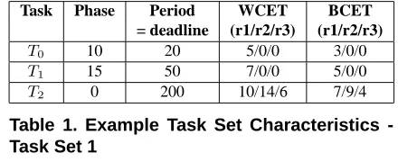
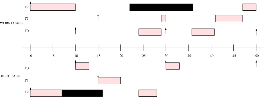
We now provide an illustrative example of our method-ology. In our example, we use a task set with three tasks whose characteristics are specified in Table 1. The first col-umn shows the task name. The second and third colcol-umns show the phase and period (equal to the deadline) of the each task. The fourth and fifth columns show the WCETs and BCETs of each of the three regions of each task. Let us assume that the Rate Monotonic (RM) scheduling policy is used for this task set. Figure 1 shows the best and worst-case scenarios for the tasks below and above the horizon-tal time axis, respectively. The arrows show release points of the three tasks. The lightly shaded rectangles represent preemptive execution regions and the black rectangles non-preemptive regions.
Task Phase Period WCET BCET = deadline (r1/r2/r3) (r1/r2/r3)
T0 10 20 5/0/0 3/0/0
T1 15 50 7/0/0 5/0/0
T2 0 200 10/14/6 7/9/4
Table 1. Example Task Set Characteristics -Task Set 1
T0 T1 T2
T0
T1
T2
50 45
40 35
30 25
20 15
10 5
0 WORST CASE
BEST CASE
Figure 1. Best and Worst-Case Scenarios for Task Set 1
the basic concept behind our methodology. Let us con-sider all the events that would occur at time10. Job J0,0
is released. The best case for J0,0 is that it is
sched-uled immediately since there is a chance that J2,0 has
not yet started executing its NPR. It is scheduled to fin-ish region 1 at time13. On the other hand, since there is a chance that J2,0 has started its NPR, J0,0 has to wait
for at most 14 units of time (worst-case remaining exe-cution time ofJ2,0’s NPR) and is scheduled to start only
at time24. The best case for J2,0 is that it continues
ex-ecuting its NPR. However, in the worst case, since there is a chance that it has not started its NPR, it gets pre-empted byJ0,0and it now re-scheduled to start its NPR at
time15(adding the WCET ofJ0,0). However, due to the
re-lease of another higher-priority job, namely,J1,0, at time 15,J2,0 gets re-scheduled once again to start at time 22
(adding the WCET ofJ1,0).
Let us now move forward in the timeline to time22. In the worst case, this is the time at whichJ2,0 starts
execut-ing its NPR. It is scheduled to finish this region at time36. At time24,J0,0starts executing region 1 in its worst case.
It is scheduled to finish at time29. Now, consider the events that occur at time30. JobJ0,1is released. In the best case, it
starts executing region 1 right away and is scheduled to fin-ish at time 33. However, in the worst case, since J2,0 is
guaranteed to have started its NPR, J0,1 has to wait
un-tilJ2,0completes its NPR and is, hence, scheduled at time 36.
The analysis proceeds in a similar fashion until the hy-perperiod of the task set, namely200. In this example, for the sake of simplicity, preemption delay calculations are not shown. Delay at every resumption point is assumed to be zero. These calculations will be explained later in Section 4.3.
4.2. Analysis Algorithm
An algorithm briefly describing our methodology is shown in Figure 2. Our system is built on an event hi-erarchy. Every event has a handler which performs all operations necessary on the occurrence of the particu-lar event. We have several event types, each with a pri-ority, time of occurrence and information about the task and job that the event corresponds to. The events are or-dered by time, and upon ties, by priority based on the type of event. The various events in our system, in order of pri-ority, are BCEndExec, WCEndExec, DeadlineCheck, JobRelease, BCStartExec, WCStartExec and Preemp-tionDelayPhaseEnd. The algorithm in Figure 2 describes the actions that take place when a certain event is trig-gered. In the algorithm, we describe the events in an order that follows the flow of the logic rather than based on pri-ority.
In Figure 2, we first define variables that are global to all event handlers. Variables that are local to a particular event are described with the corresponding event type. The basic flow of operations in our analysis is as follows. Stand-alone WCETs and BCETs are calculated for each region of each task. JobRelease and Deadline check events are pre-created based on task periods and inserted into a global event list. Events in the event list are handled one at a time until there are no more events. The basic life-cycle of a job is described below. Upon release of a job, we evaluate when that job gets scheduled if possible and determine whether any job that is currently executing gets preempted due to this re-lease. This triggers a B/WCStartExec event which signify the start of execution of the current region of a job. These events in turn schedule B/WCEndExec events or Preemp-tionDelayPhaseEnd events as the case may be. Finally, a DeadlineCheck is triggered and is responsible for checking if a certain job missed its deadline.
Structures global to all events are described below bc service queue, wc service queue : queues of all
released jobs that have not yet completed in the best and worst case respectively. Each job is in
one of three states : READY, WAITING and IN SERVICE event list : list of events ordered first by time and then
by the priority of the type of event Parameters for each event are described below
current time : Time at which event occurs curr job: Job which the event corresponds to
JobRelease event: This event represents the release
of a new job of a task.
Best case handling:
If (event queue is empty){
insertIntoEventList(curr job, current time, BCStartExec)
}else{
for every job (q job) in bc service queue starting from lowest priority job{
if (curr job has greater priority than q job){
check npr status of q job evaluate if q job gets preempted
evaluate start time of curr job gets in best case
}else{
curr job is not scheduled now break from for loop
} } }
insert curr job into bc service queue
Worst case handling:
If (event queue is empty){
create event←TRUE
}else{
for every job (q job) in wc service queue starting from lowest priority job{
if (curr job has greater priority than q job){
check if npr possible for q job check if npr guaranteed for q job if (q job gets preempted){
calculate preemption delay put q job in PreemptionDelay phase
}
re-schedule WCStartExec event for q job if required schedule WCStartExec event for curr job
}else{
curr job is not scheduled now break from for loop
} } }
insert curr job into wc service queue
BCStartExec event : This event represents the best case
start of execution of the current job’s current region. set status of curr job to IN SERVICE in bc service queue schedule BCEndExec event for curr job
BCEndExec event : This event represents the best case
end of execution of the current job’s current region.
remove curr job from bc service queue update bc remaining time of current job
if (curr job has another region){
evaluate if next region can be scheduled
schedule BCStartExec event for next region if possible insert curr job into bc service queue
}else if (bc service queue has more jobs in it) ){
schedule BCStartExec event of next READY job
}
WCStartExec event : This event represents the worst case
start of execution of the current job’s current region. set status of curr job to IN SERVICE in bc service queue if (curr job is in PreemptionDelay phase){
schedule PreemptionDelayPhaseEnd event for curr job
}else{
schedule WCEndExec event for curr job
}
WCEndExec event : This event represents the worst case
end of execution of the current job’s current region.
remove curr job from wc service queue update wc remaining time of curr job
if (curr job has another region){
evaluate if next region can be scheduled
schedule WCStartExec event for next region if possible insert curr job into wc service queue
}else if (wc service queue has more jobs in it) ){
schedule WCStartExec event of next READY job
}
DeadlineCheck event : This event checks whether the given
job has exceeded its deadline. if (curr job misses deadline) re-lease its structures
PreemptDelayPhaseEnd event : This event represents
the end of the preemption delay phase for the current job. schedule WCStartExec event for curr job
Main Algorithm : This is the starting point of
our analysis.
for every task in the task set{
create JobRelease events for all jobs of task create DeadlineCheck events for all jobs of task
}
while (events in event list){
get highest priority event and handle it based on event type
}
An arrow from one event type to another indicates that the handler of the first event type may create an event of the sec-ond type. Events that do not have a creator in the diagram are created at the beginning outside any of the event types.
BCStartExec Event BCEndExec Event
WCEndExec Event WCStartExec Event
JobRelease Event
PreempDelayPhaseEnd Event DeadlineCheckEvent
Figure 3. Creation Dependencies among Event Types
4.3. Preemption Delay Calculation
Preemption delay at every identified preemption point is calculated in a manner consistent with our earlier work [13]. At every preemption point, we calculate the best-case and worst-case execution times that have been available for a task for its execution. We provide these values to the static timing analyzer and obtain the earliest and latest iteration points reachable for each of these times. We then consider the highest delay in this range of iteration points as given by the access chain weights for those points. In our past work, we simply added this delay to the remaining worst-case ex-ecution time of the task and assumed that, on resumption, execution continues from the iteration where it had left off. However, this is imprecise since we do not know at what points the preemption delay is actually incurred during the execution of the task. Hence, for future preemption points, determination of the iteration range where the task is sup-posed to be when it is preempted is not guaranteed.
In order to solve the above problem and provide safe esti-mates of the worst-case preemption delay at every point, we devised the following solution. When a task is preempted, we calculate the delay as indicated above. When the task later resumes execution, it enters a preemption delay phase for a time equal to the calculated delay. In this phase, the task prefetches all data cache items that contribute to the de-lay. Once done, the task resumes normal execution. If a task gets preempted during its preemption delay phase, it pes-simistically starts the same preemption delay phase all over again once it resumes execution. This new phase ensures that all future delay calculations are accurate.
5. Experimental Results
For our experiments, we constructed several task sets us-ing benchmarks from the DSPStone benchmark suite [18], consistent with earlier work [13]. These task sets have base utilizations of 0.5, 0.6, 0.7 and 0.8. For each of these
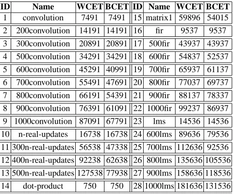
utiliza-tions, we construct task sets with 2, 4, 6 and 8 tasks. For a utilization of 0.8, we also construct a task set with 10 tasks. In all our experiments, we use a 4KB, direct-mapped data cache with a hit penalty of 1 cycle and a miss penalty of 100 cycles. The stand-alone WCETs and BCETs of the var-ious benchmarks are depicted in Table 2.
ID Name WCET BCET ID Name WCET BCET
1 convolution 7491 7491 15 matrix1 59896 54015 2 200convolution 14191 14191 16 fir 9537 9537 3 300convolution 20891 20891 17 500fir 43937 43937 4 500convolution 34291 34291 18 600fir 54837 52537 5 600convolution 45291 40991 19 700fir 65937 61137 6 700convolution 55491 47691 20 800fir 77037 69737 7 800convolution 66191 54391 21 900fir 88137 78337 8 900convolution 76391 61091 22 1000fir 99237 86937 9 1000convolution 87091 67791 23 lms 14536 14536 10 n-real-updates 16738 16738 24 600lms 89636 79536
11 300n-real-updates 56538 47338 25 700lms 112636 92536 12 400n-real-updates 92238 62638 26 800lms 135636 105536 13 500n-real-updates 127538 77938 27 900lms 158636 118536 14 dot-product 750 750 28 1000lms 181636 131536
Table 2. Stand-Alone WCETs and BCETs of DSPStone Benchmarks
In our first set of experiments, we perform response time analysis using the method presented in this paper to calcu-late the number of preemptions and the worst-case preemp-tion delay. Due to the fact that the benchmarks used in our experiments do not already have a NPR, we simply choose an iteration range from the valid iteration range of a particu-lar task and mark it as being non-preemptive. Table 3 shows execution times of each region as determined by the tim-ing analyzer based on the chosen iteration ranges for a sub-set of our benchmarks. Since we only have a fixed sub-set of benchmarks, we sometimes use the same benchmark with and without NPRs in different task sets. The length of the NPR of a task as a portion of the total execution time of the task ranges from4%to37%in both the worst and the best cases.
ID Region 1 Region 2 (NPR) Region 3 WCET / BCET WCET / BCET WCET / BCET
5 39371 / 38271 5084 / 2184 836 / 536
6 39371 / 38971 10924 / 6024 5196 / 2696
7 46771 / 44471 14224 / 7224 5196 / 2696
8 52371 / 48771 18824 / 9624 5196 / 2696
9 61571 / 55471 15424 / 7224 10096 / 5096
11 33494 / 31194 5337 / 3737 17707 / 12407
12 52294 / 43194 9647 / 4847 30297 / 14597
13 68444 / 53344 12987 / 5587 46107 / 19007 15 28912 / 26172 22400 / 20760 8584 / 7083
17 32302 / 32302 9045 / 9045 2590 / 2590
18 45802 / 45402 5845 / 4545 3190 / 2590
19 58652 / 55352 5845 / 4545 1440 / 1240
20 56502 / 53602 11545 / 9045 8990 / 7090
21 69352 / 63552 11545 / 9045 7240 / 5740
22 70152 / 64052 17245 / 13545 11840 / 9340
24 47756 / 45956 4649 / 3549 37231 / 30031
26 66506 / 60406 5239 / 3939 63891 / 41191
27 59256 / 54956 20639 / 15639 78741 / 47941
Table 3. Characteristics of Regions of Tasks with NPR
phases of the tasks are chosen in a way to demonstrate in-teresting features of our analysis.
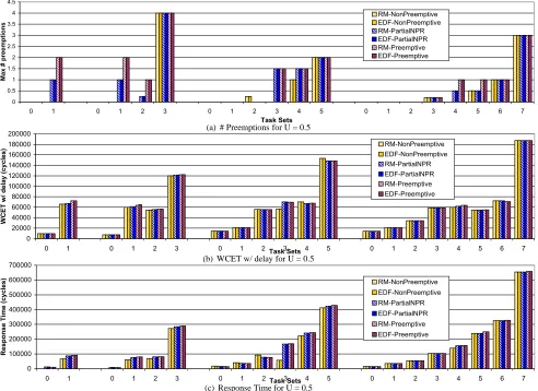
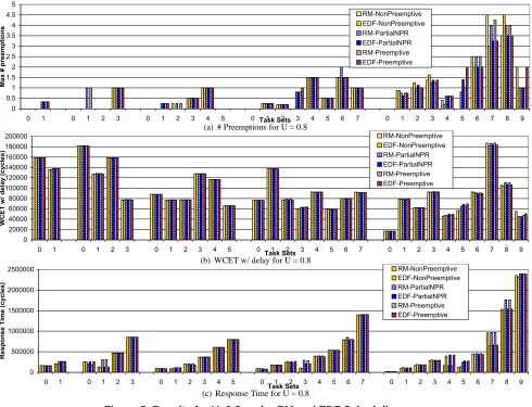
Results obtained for task sets in the above set of exper-iments are shown in Figures 4 and 5 for base utilizations of 0.5 and 0.8, respectively. Each graph shows the results of analysis of the same task sets using both the static Rate Monotonic (RM) scheduling policy and the dynamic Earli-est Deadline First (EDF) scheduling policy. The results for utilizations 0.6 and 0.7 are omitted due to space constraints. For each utilization, we have a separate graph for the max-imum number of preemptions, the WCET with preemption delay and the response time. These values form the y-axes in the graphs. In each graph, on the x-axis, we show the var-ious task sets used. Tasks within each task set are numbered from0onwards.
For each scheduling policy, we show results using three analysis techniques. The first one is NPR unaware (Preemp-tive), in which all tasks are assumed to be completely pre-emptive, as in our earlier work [13]. The second is a NPR-aware analysis in which some tasks have a non-preemptive region in the middle (PartialNPR). The third analysis is a NPR-aware analysis in which the same tasks are completely non-preemptive (NonPreemptive). In these graphs, we omit response time values for tasks that end up missing their deadline.
At the outset, it is to be noted that, if a task is supposed to have a non-preemptive region, then forcing the task to be completely preemptive is unsafe since the results of the task could be incorrect (due to possible data races). Hence, the results of our NPR unaware (Preemptive) analysis are
# Tasks 2 4 6 8
U = 0.5
IDs 16, 19N 1,
15N, 18N, 22
23, 3, 6, 11N, 19, 26
2, 3, 4, 11, 15N, 18, 7, 27
Phases 4K, 0 1K, 0, 10K, 0
32K, 32K, 32K, 0, 0, 0
0, 0, 0, 0, 0, 0, 0, 0
Periods 50K, 200K 50K, 400K, 500K, 1000K 400K, 500K, 1000K, 1000K, 2000K 100K, 400K, 500K, 800K, 1000K, 2000K, 2000K, 4000K
U = 0.6
IDs 21, 27N 1, 15,
8N, 27
3, 4, 6, 11N, 19, 26
2, 5, 6N, 11N, 15, 18, 7, 27
Phases 55K, 0 0, 0, 0, 0
32K, 33K, 34K, 0, 0, 0
0, 45K, 32K, 0, 0, 0, 0, 0
Periods 300K, 500K 50K,
400K, 500K, 1000K 100K, 400K, 500K, 1000K, 1000K, 2000K 100K, 400K, 500K, 800K, 1000K, 2000K, 2000K, 4000K
U = 0.7
IDs 27N, 21N 16, 9,
7N, 27
3, 17N, 8, 7, 20N, 27
3, 5N, 20, 11N, 15, 19, 8, 26
Phases 64K, 0 45K, 45K, 0, 0
0, 0, 0, 0, 0, 0 0, 0, 0, 0, 0, 0, 0, 0
Periods 300K, 500K 50K,
400K, 500K, 1000K 100K, 400K, 500K, 1000K, 1000K, 2000K 100K, 400K, 500K, 800K, 1000K, 2000K, 2000K, 4000K
U = 0.8
IDs 27, 26N 28,
13N, 27, 19
21, 8N, 20, 13, 25, 19
8, 26, 20, 15N, 9, 11, 8, 21
Phases 0, 0 54K, 0, 0, 0
49K, 0, 0, 0, 0, 0
27K, 27K, 27K, 0, 0, 0, 0, 0
Periods 300K, 500K 500K,
500K, 1000K, 2000K 400K, 500K, 500K, 1000K, 1000K, 2000K 400K, 500K, 800K, 800K, 1000K, 2000K, 2000K, 4000K
U = 0.8, # Tasks=10 IDs 10, 8, 15, 9, 5, 11N, 20, 27, 22, 17
Phases 32K, 32K, 32K, 32K, 32K, 0, 0, 0, 0, 0 Periods 100K, 625K, 625K, 625K, 1000K, 1000K,
1250K, 1250K, 2500K, 5000K
Table 4. Task Set Characteristics: Benchmark IDs, Phases[cycles]and Periods[cycles]
unsafe as far as the tasks with NPR are concerned. It is purely for the sake of comparison that we present those re-sults here. On the other hand, making a task that is supposed to have a portion which is preemptive completely non-preemptive is conservative, yet safe.
+B Y Y+B p p+B +B +B
Y Y p Y p B Y p B µ Ì
ú(?Vm(
²ÉVàV÷%÷<Sj(
²¯SjÆ%÷<Ý ô"¯SjÆ%÷<Ý ²Æ<9¯Æ ô"Æ<9¯Æ ²Æ%÷<Ý ô"Æ%÷<Ý
(a) # Preemptions for U = 0.5
p µ P Y Yp Y Yµ YP p
Y Y p Y pú(?Vm( B Y p B µ Ì
g~ôúV¬VÃ9ÚVñÚ9(
²¯SjÆ%÷<Ý ô"¯SjÆ%÷<Ý ²Æ<9¯Æ ô"Æ<9¯Æ ²Æ%÷<Ý ô"Æ%÷<Ý
(b) WCET w/ delay for U = 0.5
Y p B µ Ì
Y Y p Y p ú(?Vm( B Y p B µ Ì
(÷Sj(Vú<%VñÚ9(
²¯SjÆ%÷<Ý ô"¯SjÆ%÷<Ý ²Æ<9¯Æ ô"Æ<9¯Æ ²Æ%÷<Ý ô"Æ%÷<Ý
(c) Response Time for U = 0.5
Figure 4. Results for U=0.5 under RM and EDF Scheduling
First of all, we observe that the results for the RM schedul-ing policy and the EDF schedulschedul-ing policy are almost the same for most tasks. For RM and EDF to exhibit a dif-ference in behavior, a task with a longer period needs to have an earlier deadline than one with shorter period some-where in the execution timeline. This could happen in two situations, namely, when the shorter period does not divide the longer period and when there is phasing between the tasks. In most of our task sets, neither case occurs as ob-servable from the results. However, for a base utilization of 0.8, we do observe small differences in the two policies. As expected, some tasks with a shorter period (higher prior-ity according to RM) have a longer response time with EDF. Other tasks in the same task set with a longer period have a shorter response time with EDF.
For most of our task sets, we observe that the response time estimates obtained from the NonPreemptive analysis is shorter than that obtained from the PartialNPR analysis. The reason for this is as follows. In the PartialNPR analy-sis, the following situation could occur. When a task is re-leased, some task with a lower priority could have started its NPR in the best case, but not started it in the worst.
As explained in Section 4, when this happens, we con-sider the effects of contradicting worst-case scenarios for the two tasks involved. In other words, we assume the worst possible scenario for each task. This is done in order to en-sure safety of the response time estimates. In reality, how-ever, only one of the scenarios can actually occur. In the case of the NonPreemptive analysis, a task that has a NPR is assumed to be completely non-preemptive. Hence, a situ-ation like the one described above cannot occur.
On the other hand, in some task sets, the NonPreemptive analysis causes some high-priority tasks to miss their dead-lines. This is because the waiting time for the high-priority tasks are now longer since the length of the non-preemptive region of a task extends to its entire execution time. This, in part, compensates for the pessimism that the PartialNPR method introduced and is observed by the fact that the ac-tual difference between response times of tasks in the two cases are not significant.
+B Y Y+Bp p+B +B +B B
Y Y p Y p B ú(?Vm(Y p B µ Ì Y p B µ Ì P 6
²ÉVàV÷%÷<Sj(
²¯SjÆ%÷<Ý ô"¯SjÆ%÷<Ý ²Æ<9¯Æ ô"Æ<9¯Æ ²Æ%÷<Ý ô"Æ%÷<Ý
(a) # Preemptions for U = 0.8
p µ P Y Yp Y Yµ YP p
Y Y p Y p B ú(?Vm(Y p B µ Ì Y p B µ Ì P 6
g~ôúV¬VÃ9ÚVñÚ9(
²¯SjÆ%÷<Ý ô"¯SjÆ%÷<Ý ²Æ<9¯Æ ô"Æ<9¯Æ ²Æ%÷<Ý ô"Æ%÷<Ý
(b) WCET w/ delay for U = 0.8
B Y YB p pB
Y Y p Y p B ú(?Vm(Y p B µ Ì Y p B µ Ì P 6
(÷Sj(Vú<%VñÚ9(
²¯SjÆ%÷<Ý ô"¯SjÆ%÷<Ý ²Æ<9¯Æ ô"Æ<9¯Æ ²Æ%÷<Ý ô"Æ%÷<Ý
(c) Response Time for U = 0.8
Figure 5. Results for U=0.8 under RM and EDF Scheduling
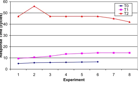
cases. We start without a NPR forT2 and then extend the
NPR from the middle outwards symmetrically in both direc-tions untilT2is completely non-preemptive. Table 5 shows
the WCETs and BCETs of each region for different experi-ments. The average response times over all jobs of each task using the RM scheduling policy are shown in Figure 6. Re-sponse times are omitted from the graph if any job of a task misses its deadline. At one extreme, whereT2is completely
preemptive, we see that the response time ofT0is the same
as its WCET since it executes to completion right after its initial release. At the other extreme, whenT2is completely
non-preemptive, we see thatT0 misses its deadline due to
increased waiting time. This sensitivity study demonstrates the improved schedulability of our PartialNPR analysis over the NonPreemptive analysis.
In summary, our work enables us to study the ef-fects of having a non-preemptive region and the ad-vantages of having partial NPRs as compared to com-pletely non-preemptive tasks in a task set. Assuming that a task is completely non-preemptive is simpler from an anal-ysis standpoint. However, it has the disadvantage that there is an increased probability that task sets are not
schedula-Expt. # Region 1 Region 2 (NPR) Region 3 WCET / BCET WCET / BCET WCET / BCET
1 30/20 0/0 0/0
2 13/9 4/2 13/9
3 11/8 8/4 11/8
4 9/7 12/6 9/7
5 7/6 16/8 7/6
6 5/4 20/12 5/4
7 3/2 24/16 3/2
8 0/0 30/20 0/0
Table 5. Execution times forT2
Y p B µ
Y p B µ Ì P
ôÉ÷<%j
(÷Sj(Vú<%VñÚ9(
ú úY úp
Figure 6. Response Times of Tasks
6. Conclusion
We presented a framework to calculate safe and tight timing bounds of data-cache related preemption de-lay (D-CRPD) and worst-case response times. In con-trast to past work, our novel approach handles tasks with a non-preemptive region of execution. Through exper-iments, we obtain response-time bounds for task sets where some tasks have non-preemptive regions. We com-pare these results to an equivalent task set where only those tasks with non-preemptive regions are sched-uled non-preemptively altogether. We show that, for some task sets, schedulability is improved without signifi-cantly affecting the response times of tasks using partially non-preemptive tasks as opposed to fully non-preemptive tasks. To the best of our knowledge, this is the first frame-work that bounds D-CRPD and response times for tasks with non-preemptive regions.
References
[1] S. Chatterjee, E. Parker, P. Hanlon, and A. Lebeck. Exact analysis of the cache behavior of nested loops. In ACM
SIG-PLAN Conference on Programming Language Design and Implementation, pages 286–297, June 2001.
[2] B. B. Fraguela, R. Doallo, and E. L. Zapata. Automatic ana-lytical modeling for the estimation of cache misses. In
Inter-national Conference on Parallel Architectures and Compila-tion Techniques, 1999.
[3] S. Ghosh, M. Martonosi, and S. Malik. Cache miss equa-tions: a compiler framework for analyzing and tuning mem-ory behavior. ACM Transactions on Programming Lan-guages and Systems, 21(4):703–746, 1999.
[4] L. Ju, S. Chakraborty, and A. Roychoudhury. Accounting for cache-related preemption delay in dynamic priority schedu-lability analysis. In IEEE Design Automation and Test in
Eu-rope, 2007.
[5] S. Kim, S. Min, and R. Ha. Efficient worst case timing anal-ysis of data caching. In IEEE Real-Time Embedded
Technol-ogy and Applications Symposium, June 1996.
[6] C.-G. Lee, J. Hahn, Y.-M. Seo, S. L. Min, R. Ha, S. Hong, C. Y. Park, M. Lee, and C. S. Kim. Analysis or cache-related
preemption delay in fixed-priority preemptive scheduling.
IEEE Transactions on Computers, 47(6):700–713, 1998.
[7] C.-G. Lee, K. Lee, J. Hahn, Y.-M. Seo, S. L. Min, R. Ha, S. Hong, C. Y. Park, M. Lee, and C. S. Kim. Bounding cache-related preemption delay for real-time systems. IEEE
Trans-actions on Software Engineering, 27(9):805–826, Nov. 2001.
[8] Y.-T. S. Li, S. Malik, and A. Wolfe. Cache modeling for real-time software: Beyond direct mapped instruction caches. In
IEEE Real-Time Systems Symposium, pages 254–263, Dec.
1996.
[9] S.-S. Lim, Y. H. Bae, G. T. Jang, B.-D. Rhee, S. L. Min, C. Y. Park, H. Shin, and C. S. Kim. An accurate worst case tim-ing analysis for RISC processors. In IEEE Real-Time
Sys-tems Symposium, pages 97–108, Dec. 1994.
[10] T. Lundqvist and P. Stenstrm. Empirical bounds on data caching in high-performance real-time systems. Technical report, Chalmers University of Technology, 1999.
[11] H. Ramaprasad and F. Mueller. Bounding worst-case data cache behavior by analytically deriving cache reference pat-terns. In IEEE Real-Time Embedded Technology and
Appli-cations Symposium, pages 148–157, Mar. 2005.
[12] H. Ramaprasad and F. Mueller. Bounding preemption de-lay within data cache reference patterns for real-time tasks. In IEEE Real-Time Embedded Technology and Applications
Symposium, Apr. 2006.
[13] H. Ramaprasad and F. Mueller. Tightening the bounds on feasible preemption points. In IEEE Real-Time Systems
Sym-posium, pages 212–222, Dec. 2006.
[14] J. Staschulat and R. Ernst. Multiple process execution in cache related preemption delay analysis. In ACM
Interna-tional Conference on Embedded Software, 2004.
[15] J. Staschulat and R. Ernst. Worst case timing analysis of in-put dependent data cache behavior. In Euromicro Conference
on Real-Time Systems, 2006.
[16] J. Staschulat, S. Schliecker, and R. Ernst. Scheduling anal-ysis of real-time systems with precise modeling of cache re-lated preemption delay. In Euromicro Conference on
Real-Time Systems, 2005.
[17] R. T. White, F. Mueller, C. Healy, D. Whalley, and M. G. Harmon. Timing analysis for data and wrap-around fill caches. Real-Time Systems, 17(2/3):209–233, Nov. 1999. [18] V. Zivojnovic, J. Velarde, C. Schlager, and H. Meyr.
Dsp-stone: A dsp-oriented benchmarking methodology. In Signal