Building Structures Under Pressurization of High Energy Line Break –
Non-Linear Analysis Method
Taha D. AL-Shawaf1
1
Manager, Material and Structural Analysis, AREVA NP Inc., Naperville, IL
ABSTRACT
Compartment pressurization is considered an impulse load since it is a transient (time varying) load determined by an external source and is relatively insensitive to structural response. Linear methods such as calculating the Dynamic Load Factor (DLF) may not be sufficient to qualify existing structures. The yield line/plastic hinge method is used to evaluate the components beyond the yield point. The multi-degree of freedom system is transformed into an equivalent single degree of freedom system. A numerical method using predictor-corrector algorithm is used to solve the elastic-plastic problem using spread sheet software. Ductility and hinge rotation are checked to ensure that the component can withstand the large deformation. The elastic-plastic method was used to qualify structural components that could not pass using the linear elastic methods thus avoiding costly modifications.
INTRODUCTION
Design Basis Specifications for most nuclear power plants require that rooms or compartments that are affected by the post accident pressure of a high energy line break (HELB) are designed and constructed to minimize or resist this pressure. An evaluation of the various structural components in any given room is required for the pressure transient that is exerted in that room. Recently some utilities have-re-evaluated this loading due to revised predicted failure pressure of blowout panels, increased pressure due to power uprate or new steam generator installation.
Compartment pressurization is considered an impulse load since it is a transient (time varying) load determined by an external source and is relatively insensitive to structural response. Linear methods such as calculating the DLF, as described in References [1] and [2], may not be sufficient to qualify existing structures. The yield line/plastic hinge method is used to evaluate the structural components beyond the yield point. This method uses a yield-line (collapse mechanism) approach to obtain the ultimate load of the component. Ductility and hinge rotation are checked to ensure that the component can withstand the large deformation.
METHODOLOGY
The capacity of a component can be determined by calculating the pressure that will cause a plastic collapse mechanism. For a plate (e.g., a slab), this requires finding a plastic yield line pattern that produces the minimum energy. This internal resistance energy is equated to the external work and thus the applied pressure to cause failure can be determined. Many slabs are designed (by virtue of their steel reinforcement) to be one-way slabs. Hence, these slabs can be modeled as a beam of width equals to unity. This will simplify the problem and reduces it to a plastic hinge-mechanism evaluation.
The approach used in this evaluation is based on the method described in References [3] and [4]. The method transforms the multi-degree of freedom (MDOF) system (e.g., slab or beam) into a single degree of freedom (SDOF) system and use numerical integration to solve the non-linear dynamic problem.
Converting MDOF to SDOF
To convert a MDOF system into a dynamically equivalent SDOF system, it is necessary to evaluate the parameters
of the system: namely, the equivalent mass, ME, the equivalent spring constant, KE, and the equivalent load, FE. The
equivalent system is selected usually so that the deflection of the concentrated mass is the same as that for a significant portion of the structure. The dynamic deflected shape of the structure is taken as the shape resulting from the static application of the dynamic loads. Load, mass, and resistance transformation factors are introduced to simplify the process of
conversion. This method is presented in Reference [3]and is summarized here for convenience.
With FE being the equivalent force and F as the applied dynamic force, the load factor, KL, is defined as:
KL = FE/F (1)
The load factor is derived by setting the external work done by the equivalent load, FE, on the equivalent system
equal to the external work done by the actual load, F, on the actual element deflecting to the assumed deflected shape. With
ME being the mass of the equivalent system and M as the total mass of the actual system, the mass factor, KM, is defined as:
KM = ME/M (2)
The mass factor is derived by setting the kinetic energy of the equivalent system equal to the kinetic energy of the
actual structure as determined from the deflected shape. Values of KL and KM for one-way elements were derived and
presented in Reference [3]. With RE being the resistance (restoring force) of the equivalent system and R as the total
resistance of the structural element, the resistance factor, KR, is defined as:
KR = RE/R (3)
To obtain the resistance factor, the strain energy of the equivalent system is equated to the strain energy of the structural element, as computed from the assumed deflected shape. Since the resistance of an element is the internal force
tending to restore the element to its unloaded static position, it can be shown that the resistance factor, KR, must always equal
the load factor, KL.
The load-mass factor is a factor formed by combining the two basic transformation factors, KL and KM. The
equation of motion of the actual system neglecting damping is given as:
F – R = Ma (4)
And for the equivalent system
KLF – KLR = KMMa (5)
Which can be re-written as
F – R = (KM/KL)Ma (6)
Or F – R = KLMMa = Mea (7)
where
KLM = the load-mass factor = KM/KL Me = effective total mass of the equivalent system
A sample of KL, KM, and KLM values for one-way elements is shown in Table 1.
Table 1. Transformation Factors for One-Way Elements, [3]
Configuration Range of
behavior
Load Factor
KL
Mass Factor
KM
Load-Mass Factor
KLM
Elastic 0.64 0.50 0.78
Plastic 0.50 0.33 0.66
Elastic 0.58 0.45 0.78
Elasto-Plastic 0.64 0.50 0.78
Plastic 0.50 0.33 0.66 Elastic 0.53 0.41 0.77
Elasto-Plastic 0.64 0.50 0.78
Plastic 0.50 0.33 0.66 Elastic 0.40 0.26 0.65
Hence, a multi-degree of freedom (MDOF) system can be transformed into a single degree of freedom (SDOF) system that can be solved with ease.
ELASTIC-PLASTIC ANALYSIS OF A SDOF SYSTEM
The equation of motion for an elastic single degree of freedom system can be written as:
F – kx – cv = ma (8)
where:
F = applied force k = stiffness of the system x = displacement c = damping
v = velocity m = mass a = acceleration
This equation can be re-written for an elastic-plastic single degree of freedom system by including the restoring force R instead of the term kx.
F – R – cv = ma (9)
Using the average acceleration method, the velocity and displacement is expressed as:
vt = vt-1 +1/2(at + at-1)Δt (10)
xt = xt-1 +1/2(vt + vt-1)Δt (11)
Substituting Eq. (10) into Eq. (9) and rearranging,
⎥ ⎦ ⎤ ⎢
⎣ ⎡
⎟ ⎠ ⎞ ⎜
⎝
⎛ +
− − Δ +
= − −
2
Δt a v c R F
2 t c m
1
at t 1 t 1 (12)
The term R is non-linear and depends on the displacement x at time t. To solve this problem numerically, a predictor-corrector method is utilized[3]. In this method the displacement x at time t is estimated (predicted) and then
corrected. A convergence of this procedure can be obtained in a single iteration if the value of Δt is small enough. A
recommended value for Δt is < T/10, where T is the period of the structure. The following step-by-step procedure is used:
1. At t = 0, compute at (t = t0) from Eq. (9) and the initial conditions
2. Increment time: t = t + Δt
3. At t = t + Δt, set at = at-1 (t-1 = 0, initially)
4. Compute vt and xt from Eqs. (10) and (11)
5. Compute R
6. Compute at from Eq. 12
If this is the predicting pass, return to Step 4. If this is the correcting pass, set xt-1 = xt, vt-1 = vt, at = at-1, and return to
Step 2.
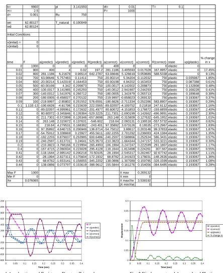
This method was implemented using a spread sheet program. The results of the response of the SDOF system to a triangular forcing function is shown on Table 2 and Figure 1. The triangular forcing function is maximum at time zero and decreases linearly to zero at T=0.1 sec. Note that in Table 2, the data between time points 0.2 and 0.4 sec are hidden to save
publication space. With TN being the natural period of the structure, Ru as the ultimate resistance, P as the peak pressure,
T/TN= 0.1/0.1= 1.0, Ru/P= 750/1000= 0.75 and the resulting ductility is calculated to be Xm/XE = 3.54 where Xm and XE are
the maximum and elastic displacement respectively. The maximum displacement occurs at tm=0.08 sec, i.e., tm/T= 0.8. These results match the results reported on Figures 3-54 and 3-55 of Reference [3].
Table 2. SDOF Elastic-Plastic Solution for Triangular Forcing Function
k= 9860 pi 3.141593 dt= 0.01 T= 0.1
m= 2.5 P= 1000
d= 0.001 Ru 750
wn 62.80127 T_natural 0.100049
wd 62.80124
Initial Conditions
v(initial) = 0
x(initial) 0
time F a(predict) v(predict) x(predict) R(predict) a(correct) v(correct) x(correct) R(correct) state xp(plastic)
% change in x
0 1000 0 0 0 0 400 0 0 0 elastic 0
0.01 900 400 4 0.02 197.2 281.1186 3.405593 0.017028 167.8957 elastic 0 17.45%
0.02 800 281.1186 6.21678 0.06514 642.2787 63.08646 5.126619 0.059689 588.5338 elastic 0 9.13%
0.03 700 63.08646 5.757483 0.11411 750 -20.00214 5.34204 0.112032 750 plastic 0.035967 1.85%
0.04 600 -20.00214 5.142019 0.164453 750 -60.00198 4.94202 0.163453 750 plastic 0.087388 0.61%
0.05 500 -60.00198 4.342 0.209873 750 -100.0017 4.142002 0.208873 750 plastic 0.132808 0.48%
0.06 400 -100.0017 3.141985 0.245293 750 -140.0012 2.941987 0.244293 750 plastic 0.168228 0.41%
0.07 300 -140.0012 1.541976 0.266712 750 -180.0005 1.341979 0.265713 750 plastic 0.189648 0.38%
0.08 200 -180.0005 -0.458027 0.270132 750 -219.9997 -0.658023 0.269132 750 plastic 0.193067 0.37%
0.09 100 -219.9997 -2.85802 0.251552 576.6591 -190.6626 -2.711334 0.252286 583.8907 elastic 0.193067 0.29%
0.1 1.11E-13 -190.6626 -4.61796 0.215639 222.5565 -89.02097 -4.109752 0.21818 247.6112 elastic 0.193067 1.16%
0.11 0 -89.02097 -4.999961 0.172632 -201.4977 80.60072 -4.151853 0.176872 -159.6859 elastic 0.193067 2.40%
0.12 0 80.60072 -3.345846 0.139384 -529.3225 211.7301 -2.690199 0.142662 -496.9991 elastic 0.193067 2.30%
0.13 0 211.7301 -0.572898 0.126346 -657.8698 263.148 -0.315809 0.127632 -645.1952 elastic 0.193067 1.01%
0.14 0 263.148 2.315672 0.137631 -546.602 218.64 2.093131 0.136518 -557.5732 elastic 0.193067 0.82%
0.15 0 218.64 4.279531 0.168382 -243.401 97.35892 3.673126 0.16535 -273.2967 elastic 0.193067 1.83%
0.16 0 97.35892 4.646715 0.206949 136.8714 -54.75012 3.88617 0.203146 99.37653 elastic 0.193067 1.87%
0.17 0 -54.75012 3.338669 0.23927 455.5611 -182.2255 2.701292 0.236083 424.1384 elastic 0.193067 1.35%
0.18 0 -182.2255 0.879037 0.253985 600.6486 -240.2597 0.588866 0.252534 586.3431 elastic 0.193067 0.57%
0.19 0 -240.2597 -1.813731 0.24641 525.9573 -210.3823 -1.664344 0.247157 533.3221 elastic 0.193067 0.30%
0.2 0 -210.3823 -3.768166 0.219994 265.4993 -106.1984 -3.247247 0.222599 291.1807 elastic 0.193067 1.17%
0.4 0 -167.4715 -2.060034 0.223028 295.4128 -118.1644 -1.813498 0.224261 307.567 elastic 0.193067 0.55%
0.41 0 -118.1644 -2.995142 0.200218 70.50105 -28.1994 -2.545317 0.202467 92.67742 elastic 0.193067 1.11%
0.42 0 -28.1994 -2.827311 0.175604 -172.1932 68.8782 -2.341923 0.178031 -148.2635 elastic 0.193067 1.36%
0.43 0 68.8782 -1.653141 0.158055 -345.2202 138.0886 -1.307089 0.159785 -328.1599 elastic 0.193067 1.08%
0.44 0 138.0886 0.073797 0.153619 -388.9612 155.5844 0.161276 0.154056 -384.6485 elastic 0.193067 0.28%
Max F 1000 X max 0.269132
Min F 0 X min 0
Xe 0.076065 X max/Xe 3.538192
|X min/Xe| 0
-800 -600 -400 -200 0 200 400 600 800 1000 1200
0 0.05 0.1 0.15 0.2 0.25 0.3 0.35 0.4
Time (sec)
F
o
rce,
A
c
cel
er
ati
o
n
,
R
es
ist
an
ce
F a(predict) R(predict) a(correct) R(correct)
Fig. 1 Acceleration and Resistance Due to a Triangular Forcing Function
0 0.05 0.1 0.15 0.2 0.25 0.3
0 0.05 0.1 0.15 0.2 0.25 0.3 0.35 0.4
Time (sec)
D
isp
la
cem
e
n
t
x(predict) x(correct) xp(plastic) % change in x
APPLICATION
A spread sheet similar to that shown on Table 2 was created for the analysis of structural components under pressurization of HELB, the following notes and rules were used:
1. The effective moment of inertia is the average of the gross and cracked moments of inertia, References [4] and [6].
The compression steel may be neglected when calculating the cracked moment of inertia.
2. The moment capacity is calculated on a step by step basis (i.e., calculating the moment that will form the first hinge,
then the second hinge, etc.) until a collapse mechanism occurs. Attention is given to the sequence, the positive and negative reinforcement, and the corresponding moment capacity values.
3. For a two-step elasto-plastic system (i.e., formation of two hinges in sequence), the three slope curve is transformed
to a two slope curve using the method described in Sections 3.13, 3.14 and 3.17 of Reference [3]. This is done by equating the area under the curve (resistance energy) for the two systems.
4. The load-mass factor is taken from Table 1. For small plastic deformations (xmax/xe < 5), KLM is taken as the average
of the elastic and plastic values. Whereas, for larger plastic deformation (xmax/xe > 5), the equivalent KLM is taken as
the plastic value, where xmax/xe = ductility[3].
5. For convenience, the equation of motion used is expressed in terms of the unit area of the element (i.e. the force
becomes pressure, etc.).
6. The dead load (DL) includes the equipment loads and is in the same direction as the pressure for a floor or in
opposite direction to the pressure for a ceiling. The load multiplier for the DL is reduced to 1.0 for the ceiling, in order to minimize the opposing force to the pressure.
7. The pressure-time history for the applicable volume/compartment is used in the analysis.
8. The initial conditions for the predictor-corrector numerical method are zero velocity and displacement.
9. The damping value corresponds to the structural component under consideration. The critical damping is
Cc = 2 m ωn, where ωn is the natural frequency (13)
For damping value corresponding to 5% of critical damping, C = 0.05Cc
10. The equation of motion is solved for the origin at the static equilibrium as opposed to the origin at the unstretched
position. The total displacement is the sum of the displacement caused by gravity and the dynamic displacement from the static equilibrium condition. The calculation of the resistance function, R, accounts for the initial stressed condition of DL and equipment load (i.e., the initial stress, whether positive or negative, is algebraically added to the stress caused by dynamic load).
11. The stress state (i.e., elastic or plastic) is monitored and updated at each time step. The plastic displacement is
accumulated accordingly.
12. The plastic displacement is equal to the shift in the origin of the stress-strain curve in the subsequent unloading from
the plastic state and reloading of the system. Hence, the equation for the resistance, R, is defined as follows:
If (xi + DL/k – xpi-1) > 0.0 (loading)
R = Minimum of [{ k(xi-xpi-1) + DL} or Ru] (14)
Else (unloading)
R = Maximum of [{ k(xi-xpi-1) + DL} or –Ru] (15)
where:
xi = the displacement at time step i
xp i-1 = the accumulated plastic displacement (deformation) at time step i-1
= the shift of the origin of the resistance curve
DL = dead load + equipment load including any load factors and accounting for sign, e.g. for ceiling
this term is negative because it opposes the pressure
13. Equation 12 is adjusted to account for the initial prestress due to DL (including equipment load and any load factor)
as follows:
⎥ ⎦ ⎤ ⎢
⎣ ⎡
⎟ ⎠ ⎞ ⎜
⎝
⎛ +
− + − Δ
+
= −
−
2
Δt a v c DL) R ( P * 1.25
2 t c m
1
at t 1 t 1 (16)
where:
1.25 P = pressure multiplied by 1.25 load factor, [6]
DL = factored dead load + equipment load
14. The convergence of the numerical method is checked by monitoring the percent change of the displacement of the corrected pass and the predicted pass as follows:
correct predict correct
x x x
Change= − (17)
This term is undefined when the displacement, xcorrect, is zero. It is also very high in the first load step since the
xpredict is zero initially.
15. The ductility is calculated as:
⎥ ⎥ ⎦ ⎤ ⎢
⎢ ⎣ ⎡
⎟ ⎟ ⎠ ⎞ ⎜
⎜ ⎝
⎛ +
⎟ ⎟ ⎠ ⎞ ⎜
⎜ ⎝
⎛ +
=
e DL max
e DL min
x x x , x
x x Max
Ductility (18)
where:
x
min=
minimum dynamic displacementxmax = maximum dynamic displacement
xDL = initial static equilibrium displacement due to DL and equipment load
xe = elasticdisplacement
16. The ductility is checked against the allowable ductility as defined in References [5]and [6].
17. The plastic hinge rotation is calculated based on the maximum total displacement xmax + xDL and is checked against
the allowable as defined in Reference [5]. Experience has shown that the results were controlled by xmax and not
xmin.
The above methodology was used to evaluate structural components that could not be evaluated using linear analysis methods. A sample of these evaluations is summarized in the following showing the changes in the results as input parameters are varied. In these evaluations, a concrete slab which acted as a one way fixed-pin beam is converted to a SDOF system. Using the unit area of the element to solve the equations of motion, the inputs used
are the following: R= 34.012 kPa/mm2 (4.933
psi/in2), Me = 0.001617 lb.sec2/in3, KE= 5.741
psi/in, and the pressure time history is multiplied by the pressure load factor of 1.25. Figure 3 shows the results of this analysis with the DL opposing the pressure and is equal to
0.868 lb/in2 and neglecting damping (0.1%).
The resistance curve show that it reached the maximum at about 0.5 sec and continues until after 0.1 sec. The accumulated plastic deformation increases during the same time frame reaching its maximum of 27.15 mm (1.069 in). The maximum displacement occurs at 0.1 sec and is equal to 52.82 mm (2.08 in). The corresponding ductility is 2.24.
-15 -5 5 15 25 35 45
0 0.1 0.2 0.3 0.4 0.5 0.6 0.7 0.8 0.9 1
Time (sec)
Pressur
e
or R
e
sistance
(kPa)
0 10 20 30 40 50 60
D
ispl
acement or
D
ef
o
rmation (mm)
Factored Pressure (kPa) Resistance (kPa) Displacement x (mm) Accum.Plastic Deformation xp (mm)
Fig. 3 Results of Pressure Transient on a Ceiling Slab
Including DL Using 0.1 % Damping
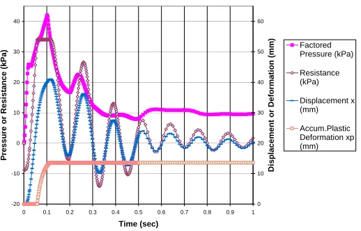
The same problem was solved using 5% damping. The results, shown on Fig. 4, exhibit a reduction of the displacement and plastic deformation. The corresponding ductility is reduced to 1.74.
Figure 5 show the solution when the maximum 1.05 (DL+LL) is used as the initial static load (prestressed condition).
The effective mass in this case is 0.002264 lb.sec2/in3. The results show, as expected, a reduction in the dynamic response
Figure 6 show the response if the DL+ LL are neglected as in the case of a reinforced concrete wall. The effective
mass of the SDOF system is 0.001617 lb.sec2/in3. The response exhibits plastic behavior at two time regions with unloading
and reloading of the structure between these regions. The ductility is calculated to be 4.27.
-10 0 10 20 30 40
0 0.1 0.2 0.3 0.4 0.5 0.6 0.7 0.8 0.9 1
Time (sec)
P
ressu
re o
r Resi
st
ance
(kP
a)
0 10 20 30 40 50
D
isp
lacemen
t
o
r D
e
fo
rmatio
n (mm
)
Factored Pressure (kPa) Resistance (kPa) Displacement x (mm) Accum. Plastic Deformation xp (mm)
Fig. 4 Results of Pressure Transient on a Ceiling Slab Including DL Using 5.0 % Damping
-20 -10 0 10 20 30 40
0 0.1 0.2 0.3 0.4 0.5 0.6 0.7 0.8 0.9 1
Time (sec)
P
ressu
re o
r Resi
st
ance
(kP
a)
0 10 20 30 40 50 60
D
isp
lacemen
t
o
r D
e
fo
rmatio
n (mm
)
Factored Pressure (kPa) Resistance (kPa) Displacement x (mm) Accum.Plastic Deformation xp (mm)
Fig. 5 Results of Pressure Transient on a Ceiling Slab Including 1.05(DL+LL) Using 5.0 % Damping
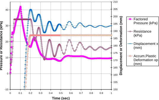
For a floor slab with 1.05(DL), the initial static load acts in the same direction as the pressure. The effective mass is
Me = 0.001483 lb.sec2/in3 and 1.05DL = 0.9114 lb/in2. Figure 7 shows high displacements in which the two plastic regions
of the previous figure are combined to form a wide plastic region. The ductility for this case is calculated to be 9.57. This example only serves as an illustration on how the initial conditions influence the results of the ductility considerably.
Hinge rotation is calculated using the geometric configuration of the collapse mechanism and the maximum displacement obtained from above. Using the non-linear analysis method makes it possible to qualify many existing structural components that cannot be qualified using the linear elastic method.
SUMMARY AND CONCLUSION
rotation are checked to ensure that the component can withstand the large deformation. The elastic-plastic method was used to qualify structural components that could not pass using the linear elastic methods thus avoiding costly modifications.
-10 0 10 20 30 40
0 0.1 0.2 0.3 0.4 0.5 0.6 0.7 0.8 0.9 1
Time (sec)
Pr
e
ssu
re o
r Resis
ta
n
ce (kPa)
0 20 40 60 80 100
D
is
p
la
ce
m
e
nt or
D
e
for
m
a
ti
on (m
m
)
Factored Pressure (kPa) Resistance (kPa) Displacement x (mm) Accum.Plastic Deformation xp (mm)
Fig. 6 Results of Pressure Transient on a Wall Neglecting DL & LL Using 5.0 % Damping
-10 0 10 20 30 40
0 0.1 0.2 0.3 0.4 0.5 0.6 0.7 0.8 0.9 1
Time (sec)
Pre
ssu
re o
r Res
ist
an
ce
(kP
a
)
150 155 160 165 170 175 180 185 190 195 200 205 210
D
isp
lac
e
m
e
n
t
or De
fo
rm
at
io
n (m
m
)
Factored Pressure (kPa)
Resistance (kPa)
Displacement x (mm)
Accum.Plastic Deformation xp (mm)
Fig. 7 Results of Pressure Transient on a Floor Slab Including 1.05DL Using 5.0 % Damping
REFERENCES
1. Biggs, J. M., Introduction to Structural Dynamics, McGraw-Hill Book Co., 1964.
2. AL-Shawaf, T. D., “Building Structures under Pressurization of High Energy Line Break – Linear Analysis,”
Structural Mechanics in Reactor Technology, SMiRT 19, Toronto , Canada, 2007.
3. Dede, M., Sock, F., Lipvin-Schramm, S. and Dobbs, N., “Structures to Resist the Effects of Accidental Explosions”-
Volume III, Principles of Dynamic Analysis, AD-148895, Ammann & Whitney, New York June 1984.
4. Dede, M. and Dobbs, N., “Structures to Resist the Effects of Accidental Explosions”, Volume IV, Reinforced Concrete
Design, AD-A178901, Ammann & Whitney, New York April 1987.
5. ASCE “Structural Analysis and Design of Nuclear Plant Facilities”, Manuals and Reports on Engineering Practice –
No. 58, American Society of Civil Engineers, New York 1980.
6. ACI 349-06 “Code Requirements for Nuclear Safety-Related Concrete Structures”, American Concrete Institute 2007.
![Table 1. Transformation Factors for One-Way Elements, [3]](https://thumb-us.123doks.com/thumbv2/123dok_us/1255009.1158118/2.612.135.476.481.675/table-transformation-factors-way-elements.webp)