An inverse problem formulation methodology for stochastic models

An Inverse Problem Formulation Methodology for Stochastic

Models

A. R. Ortiz1_{, H. T. Banks}2_{, C. Castillo-Chavez}1_{, G. Chowell}1_{, and X. Wang}1 1 _{School of Human Evolution and Social Change}

Arizona State University Tempe, Arizona 85287-2402

2_{Center for Research in Scientific Computation} North Carolina State University

Raleigh, North Carolina 27695-8212

May 2, 2010

Abstract

A method for estimating parameters in dynamic stochastic (Markov Chain) models based on Kurtz’s limit theory coupled with inverse problem methods developed for deterministic dynam-ical systems is proposed and illustrated in the context of disease dynamics. This methodology relies on finding an approximate large-population behavior of an appropriate scaled stochastic system. This approach leads to a deterministic approximation obtained as solutions of rate equations (ordinary differential equations) in terms of the large sample size average over sample paths or trajectories (limits of pure jump Markov processes). Using the resulting deterministic model we select parameter subset combinations that can be estimated using an ordinary-least-squares (OLS) or generalized-least-ordinary-least-squares (GLS) inverse problem formulation with a given data set. The selection is based on two criteria of the sensitivity matrix: the degree of sensitivity measure in the form of its condition number and the degree of uncertainty measured in the form of its parameter selection score. We illustrate the ideas with a stochastic model for the transmission of vancomycin-resistant enterococcus (VRE) in hospitals and VRE surveillance data from an oncology unit.

1

Introduction

Closely tied to the formulation of the mathematical models is the need to estimate the parameters (including initial conditions) involved as well as provide uncertainty bounds for the estimates. Validating the mathematical models with empirical data for the system under investigation is a key step in gaining insight into the system process and evaluating the effectiveness of particular control strategies [8, 10, 11, 12, 21, 24]. A number of advanced mathematical and statistical tools for parameter estimation in deterministic dynamic models are readily available. The key objective of this paper is to present a methodology to estimate parameters in a stochastic model using inverse problem methods developed for deterministic dynamical systems. In these inverse problem methods, parameter estimates along with uncertainty bounds (confidence intervals) are readily obtained from longitudinal data for a single realization of the observation process for the stochastic system. Moreover, sensitivity analysis along with parameter selection (determining which parameters are most “identifiable” with the given data) can be done without massive simulation studies.

It is difficult to carry out the above estimation related tasks directly with stochastic models and limited data. The methodology presented in this paper is based on using an approximate large-population behavior of an appropriate scaled stochastic system using Kurtz’s limit theory [19, 22]. By scaling the stochastic system and applying the Strong Law of Large Numbers (SLLN) for the relevant Poisson process, we can derive the corresponding deterministic approximation as solutions of rate equations in terms of the large sample size average over sample paths or trajectories. Using the resulting deterministic model we select parameter subset combinations that can be estimated using an ordinary-least-squares (OLS) or generalized-least-squares (GLS) inverse problem formulation with a given data set along with an appropriate statistical model for the observation process.

Given an experimental data set, a mathematical model may be more sensitive to some param-eters than others, and the dependence between the paramparam-eters can impact the well-posedness of an inverse problem. Therefore, it is of interest to limit the attempted estimation to subsets of parameters for which the mathematical model is most sensitive. The analysis used to select the type of inverse problem formulation and the subset of parameters to be estimated from a given data set is based on previous ideas in the literature [6, 14, 17], and is reviewed in Section 4. The selection procedure is based on two criteria of the sensitivity matrix: the degree of sensitivity measure in the form of its condition number and the degree of uncertainty measured in the form of its parameter selection score. The idea is to select first all parameter combinations with a full rank sensitivity matrix and then calculate the corresponding Fisher matrix condition numbers and selection scores. Then parameter subset combinations with small condition numbers and selection scores are considered as feasible (i.e., can be estimated with reasonable levels of uncertainty).

the data. In Section 4 we review the inverse problem and parameter selection methodology used to estimate parameters and quantify uncertainty for problems with deterministic systems. Finally, in Sections 5 and 6 we present some illustrative results and along with some summary conclusions.

2

A Motivating VRE Stochastic Model

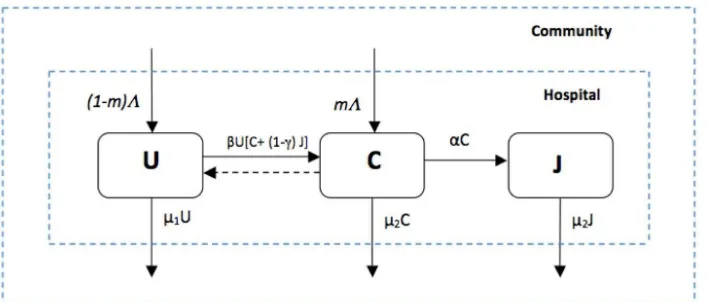
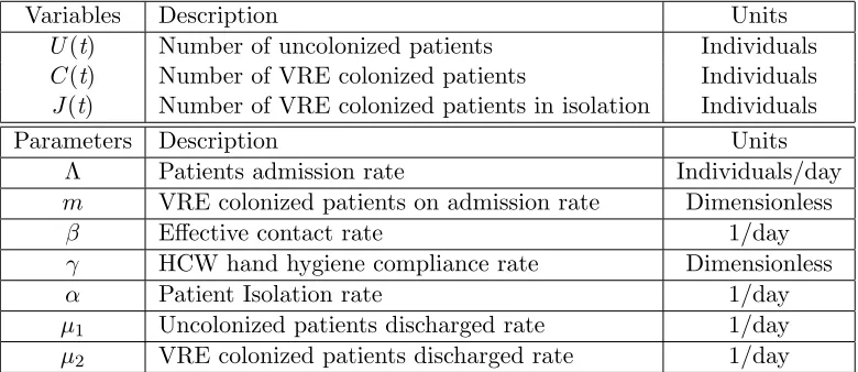
For our motivating example model, patients in a hospital unit are classified by compartments or states as either uncolonized 𝑈(𝑡), VRE colonized 𝐶(𝑡), or VRE colonized in isolation 𝐽(𝑡), as depicted in the compartmental schematic of Figure 1. A description of the variables and parameters are given in Table 1. Patients are admitted to the hospital unit at a rate Λ per day and some fraction m are already VRE colonized. The transition from one compartment to another follows an exponential distribution and the expected mean duration within a compartment is given by the inverse of the parameter of the exponential distribution. A hand-hygiene policy applied to health care workers on isolated VRE colonized patients reduces infectivity by a factor of 𝛾 (0 < 𝛾 <

1). It is assumed VRE colonization periods last from weeks to months and because spontaneous decolonization occurs infrequently, clearance of the bacteria is not considered in the model. VRE colonized patients are moved into isolation at a rate𝛼.

Figure 1: Compartmental VRE model

2.1 The VRE stochastic model

The dynamics of the VRE colonization of patients in a hospital unit are modeled as a continu-ous time Markov Chain (MC) with discrete state space [1, 5, 26] embedded in ℝ3_{. In this case,} the population of patients is considered discrete (i.e., VRE colonization occurs in units of whole individuals) and the timing of events is a probabilistic process. The state of the MC at timet is denoted by {𝑈(𝑡) = 𝑖, 𝐶(𝑡) = 𝑗, 𝐽(𝑡) = 𝑘},t ≥ 0 and 𝑖, 𝑗, 𝑘 ∈ {0,1, ...𝑁}. The probability that during a small time interval,dt, of transiting from one state to another is described by

𝑃{𝑈(t+dt) =𝑖−1, 𝐶(t+dt) =𝑗+ 1, 𝐽(t+dt) =𝑘∣𝑈(t) =𝑖, 𝐶(t) =𝑗, 𝐽(t) =𝑘}

Table 1: Model Parameters

Variables Description Units

𝑈(t) Number of uncolonized patients Individuals

𝐶(t) Number of VRE colonized patients Individuals

𝐽(t) Number of VRE colonized patients in isolation Individuals

Parameters Description Units

Λ Patients admission rate Individuals/day

𝑚 VRE colonized patients on admission rate Dimensionless

𝛽 Effective contact rate 1/day

𝛾 HCW hand hygiene compliance rate Dimensionless

𝛼 Patient Isolation rate 1/day

𝜇1 Uncolonized patients discharged rate 1/day

𝜇2 VRE colonized patients discharged rate 1/day

𝑃{𝑈(t+dt) =𝑖, 𝐶(t+dt) =𝑗+ 1, 𝐽(t+dt) =𝑘−1∣𝑈(t) =𝑖, 𝐶(t) =𝑗, 𝐽(t) =𝑘}

=𝑚𝜇2𝐽dt+o(dt), (2)

𝑃{𝑈(t+dt) =𝑖+ 1, 𝐶(t+dt) =𝑗−1, 𝐽(t+dt) =𝑘∣𝑈(t) =𝑖, 𝐶(t) =𝑗, 𝐽(t) =𝑘}

= (1−𝑚)𝜇2𝐶dt+o(dt), (3)

𝑃{𝑈(t+dt) =𝑖+ 1, 𝐶(t+dt) =𝑗, 𝐽(t+dt) =𝑘−1∣𝑈(t) =𝑖, 𝐶(t) =𝑗, 𝐽(t) =𝑘}

= (1−𝑚)𝜇2𝐽dt+o(dt), (4)

𝑃{𝑈(t+dt) =𝑖, 𝐶(t+dt) =𝑗−1, 𝐽(t+dt) =𝑘+ 1∣𝑈(t) =𝑖, 𝐶(t) =𝑗, 𝐽(t) =𝑘}

=𝛼𝐶dt+o(dt), (5)

𝑃{𝑈(t+dt) =𝑖, 𝐶(t+dt) =𝑗, 𝐽(t+dt) =𝑘∣𝑈(t) =𝑖, 𝐶(t) =𝑗, 𝐽(t) =𝑘}

= (1−𝑚)𝜇1𝑈dt+𝑚𝜇2𝐶dt+ [1−(Λ +𝛽𝑈[𝐶+ (1−𝛾)𝐽] +𝛼𝐶)]dt+o(dt). (6)

In the VRE epidemic model a constant population is assumed in which the hospital remains full for all t (i.e., overall admission rate equals overall discharge rate, Λ =𝜇1𝑈 +𝜇2(𝐶+𝐽)). Hence, the admission of a patient in either compartments𝑈 or𝐶 are dependent events on the discharged in either compartment 𝑈 or𝐶 or𝐽 (or vice versa). We assume that when a patient is discharged from the hospital, he/she is immediately replaced by an admission into the compartment 𝑈 with probability (1−𝑚) or into the compartment𝐶with probability𝑚. Equation (1) is the probability of entering compartment 𝐶 by either an admission (due to a discharge in compartment 𝑈) or by effective colonization. Equation (2) is the probability of entering compartment𝐶 by an admission due to a discharge in 𝐽. Equation (3) is the probability of admission to compartment 𝑈 by a discharge in 𝐶. Equation (4) is the probability of admission into compartment 𝑈 by a discharge in 𝐽. Equation (5) is the probability of moving a VRE colonized patient into isolation. Finally, Equation (6) is the probability that none of the states changes due to: an uncolonized patient being discharged and replaced back into the 𝑈 compartment, or a VRE colonized patient in 𝐶

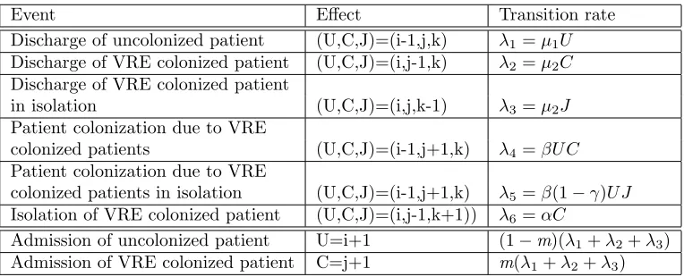
Table 2: Transition rates

Event Effect Transition rate

Discharge of uncolonized patient (U,C,J)=(i-1,j,k) 𝜆1=𝜇1𝑈

Discharge of VRE colonized patient (U,C,J)=(i,j-1,k) 𝜆2=𝜇2𝐶

Discharge of VRE colonized patient

in isolation (U,C,J)=(i,j,k-1) 𝜆3=𝜇2𝐽

Patient colonization due to VRE

colonized patients (U,C,J)=(i-1,j+1,k) 𝜆4=𝛽𝑈 𝐶

Patient colonization due to VRE

colonized patients in isolation (U,C,J)=(i-1,j+1,k) 𝜆5=𝛽(1−𝛾)𝑈 𝐽

Isolation of VRE colonized patient (U,C,J)=(i,j-1,k+1)) 𝜆6=𝛼𝐶

Admission of uncolonized patient U=i+1 (1−m)(𝜆1+𝜆2+𝜆3)

Admission of VRE colonized patient C=j+1 m(𝜆1+𝜆2+𝜆3)

2.2 The deterministic approximation

When dividing equations (1)-(6) by dt and taking the limit when dt tends to 0+, we obtain the rates of transitions as summarized in Table 2. In the stochastic model, the rates represent the mean number of transitions that can be expected in a given period, with the actual numbers distributed about these means. Hence, the rates determine the frequencies of occurrence through time for the transitions or events.

Letting 𝑅𝑖(t) for 𝑖= 1, ...,6, be the number of times the 𝑖𝑡ℎ transition has occurred by timet.

Then, the state of the system at timet can be written as

𝑈(𝑡) = 𝑈(0)−𝑅1(𝑡)−𝑅4(𝑡)−𝑅5(𝑡) + (1−𝑚)(𝑅1(𝑡) +𝑅2(𝑡) +𝑅3(𝑡))

𝐶(𝑡) = 𝐶(0)−𝑅2(𝑡) +𝑅4(𝑡) +𝑅5(𝑡)−𝑅6(𝑡) +𝑚(𝑅1(𝑡) +𝑅2(𝑡) +𝑅3(𝑡))

𝐽(𝑡) = 𝐽(0)−𝑅₃(𝑡) +𝑅₆(𝑡), (7)

where𝑅𝑖(𝑡) is a counting process with intensity𝜆𝑖(𝑈(𝑡), 𝐶(𝑡), 𝐽(𝑡)) given by

𝑅𝑖(𝑡) =𝑌𝑖

(∫ _𝑡

0

𝜆𝑖(𝑈(𝑠), 𝐶(𝑠), 𝐽(𝑠))𝑑𝑠

)

, 𝑖= 1, ...,6, (8)

with𝑌𝑖as independent unit Poisson processes. Note that the state of the system is (𝑈(𝑠), 𝐶(𝑠), 𝐽(𝑠))

and hence each 𝜆𝑖(𝑈(𝑠), 𝐶(𝑠), 𝐽(𝑠)) is constant between transition times. Also, note that sample

paths𝑟_𝑖(𝑡) of 𝑅_𝑖(t) are given in terms of sample paths (𝑢(𝑡), 𝑐(𝑡), 𝑗(𝑡)) of (𝑈(𝑡), 𝐶(𝑡), 𝐽(𝑡)) by

𝑟_𝑖(𝑡) =𝑌_𝑖

(∫ _𝑡

0

𝜆_𝑖(𝑢(𝑠), 𝑐(𝑠), 𝑗(𝑠))𝑑𝑠

)

, 𝑖= 1, ...,6. (9)

Let𝑈𝑁_{(𝑡) =𝑈(𝑡)/𝑁,𝐶}𝑁_{(𝑡) =𝐶(𝑡)/𝑁,𝐽}𝑁_{(𝑡) =𝐽(𝑡)/𝑁 be the patient units per system size or}

We express the rates𝜆𝑖 for𝑖= 1, ...,6 in terms of these scaled variables as follows:

𝜆1 =𝜇1𝑢(𝑡) =𝑁 𝜇1𝑢𝑁(𝑡), 𝜆4 =𝛽𝑢(𝑡)𝑐(𝑡) =𝑁2𝛽𝑢𝑁(𝑡)𝑐𝑁(𝑡),

𝜆2 =𝜇2𝑐(𝑡) =𝑁 𝜇2𝑐𝑁(𝑡), 𝜆5 =𝛽(1−𝛾)𝑢(𝑡)𝑗(𝑡) =𝑁2𝛽(1−𝛾)𝑢𝑁(𝑡)𝑗𝑁(𝑡),

𝜆3 =𝜇2𝑗(𝑡) =𝑁 𝜇2𝑗𝑁(𝑡), 𝜆6 =𝛼𝑐(𝑡) =𝑁 𝛼𝑐𝑁(𝑡).

Using these rates we can obtain an approximation for𝑟𝑁_𝑖 (𝑡), the averages of the𝑟𝑖(𝑡) of (9) by

apply-ing the SLLN for the Poisson Process (i.e.,𝑌(𝑁 𝜇)/𝑁 ≈𝜇). The process results in approximating for large 𝑁, the sample paths (𝑢𝑁_{(𝑡), 𝑐}𝑁_{(𝑡), 𝑗}𝑁_{(𝑡)) by a large sample size average approximation}

over paths (¯𝑢(𝑡),𝑐¯(𝑡),¯𝑗(𝑡)) defined by a deterministic system. That is, we approximate integrals in the averaged sample path equations by integrals that are used as the defining equations for the deterministic sample paths. This is done by the approximations

𝑟₁𝑁(𝑡) = 𝑟1(𝑡)

𝑁 =

1

𝑁𝑌1

(∫ _𝑡

0

𝜆1(𝑢(𝑠))𝑑𝑠

)

= 1

𝑁𝑌1

(

𝑁

∫ _𝑡

0

𝜇1𝑢𝑁(𝑠)𝑑𝑠

)

≈ 1

𝑁𝑌1

(

𝑁

∫ _𝑡

0

𝜇1𝑢¯(𝑠)𝑑𝑠

)

≈

∫ _𝑡

0

𝜇1𝑢¯(𝑠)𝑑𝑠. (10)

The approximations for𝑟𝑁

𝑖 (𝑡) for𝑖= 2, ...,6, can be obtained similarly. When dividing both sides

of the sample path analogue of each equation in (7) by N and applying the approximations for

𝑟_𝑖𝑁(𝑡), we can write the system of integral equations (i.e., rate equations) that approximate the stochastic equations (7) via the SLLN. The rate approximation equations are given by

𝑢𝑁(𝑡) =𝑢𝑁(0)−𝑟𝑁₁ (𝑡)−𝑟₄𝑁(𝑡)−𝑟₅𝑁(𝑡) + (1−𝑚)(𝑟₁𝑁(𝑡) +𝑟𝑁₂ (𝑡) +𝑟₃𝑁(𝑡))

≈𝑢¯(0)−

∫ _𝑡

0

𝜇1𝑢¯(𝑠)𝑑𝑠−

∫ _𝑡

0

𝑁 𝛽𝑢¯(𝑠)¯𝑐(𝑠)𝑑𝑠−

∫ _𝑡

0

𝑁 𝛽(1−𝛾)¯𝑢(𝑠)¯𝑐(𝑠)𝑑𝑠

+

∫ _𝑡

0

(1−𝑚)(𝜇₁𝑢¯(𝑠) +𝜇₂(¯𝑐(𝑠) + ¯𝑗(𝑠)))𝑑𝑠

𝑐𝑁(𝑡) =𝑐𝑁(0)−𝑟𝑁₂ (𝑡) +𝑟₄𝑁(𝑡) +𝑟𝑁₅ (𝑡)−𝑟₆𝑁(𝑡) +𝑚(𝑟𝑁₁ (𝑡) +𝑟₂𝑁(𝑡) +𝑟𝑁₃ (𝑡))

≈𝑐¯(0)−

∫ _𝑡

0

𝜇2¯𝑐(𝑠)𝑑𝑠+

∫ _𝑡

0

𝑁 𝛽𝑢¯(𝑠)¯𝑐(𝑠)𝑑𝑠+

∫ _𝑡

0

𝑁 𝛽(1−𝛾)¯𝑢(𝑠)¯𝑗(𝑠)𝑑𝑠

− ∫ _𝑡 0 𝛼𝑐¯(𝑠)𝑑𝑠+ ∫ _𝑡 0

𝑚(𝜇1𝑢¯(𝑠) +𝜇2(¯𝑐(𝑠) + ¯𝑗(𝑠)))𝑑𝑠

𝑗𝑁(𝑡) =𝑗𝑁(0)−𝑟₃𝑁(𝑡) +𝑟𝑁₆ (𝑡)

≈¯𝑗(0)−

∫ _𝑡

0

𝜇2¯𝑗(𝑠)𝑑𝑠+

∫ _𝑡

0

𝛼𝑐¯(𝑠)𝑑𝑠. (11)

Upon approximating (𝑢𝑁_{(𝑡), 𝑐}𝑁_{(𝑡), 𝑗}𝑁_{(𝑡)) in the left side by (¯𝑢(𝑡),𝑐¯(𝑡),¯𝑗(𝑡)) and differentiating}

given by

𝑑𝑢¯(𝑡)

𝑑𝑡 =−𝜇1𝑢¯(𝑡)−𝛽𝑁𝑢¯(𝑡)¯𝑐(𝑡)−𝛽𝑁(1−𝛾)¯𝑢(𝑡)¯𝑗(𝑡) + (1−𝑚)(𝜇1𝑢¯(𝑡) +𝜇2(¯𝑐(𝑡) + ¯𝑗(𝑡))) 𝑑¯𝑐(𝑡)

𝑑𝑡 =−𝜇2¯𝑐(𝑡) +𝛽𝑁𝑢¯(𝑡)¯𝑐(𝑡) +𝛽𝑁(1−𝛾)¯𝑢(𝑡)¯𝑗(𝑡)−𝛼𝑐¯(𝑡) +𝑚(𝜇1𝑢¯(𝑡) +𝜇2(¯𝑐(𝑡) + ¯𝑗(𝑡))) 𝑑¯𝑗(𝑡)

𝑑𝑡 =−𝜇2¯𝑗(𝑡) +𝛼𝑐¯(𝑡), (12)

with initial conditions ¯𝑢(0) =𝑈₀/𝑁, ¯𝑐(0) =𝐶₀/𝑁, and ¯𝑗(0) =𝐽₀/𝑁.

To facilitate comparison with the MC model, we let ¯𝑈(𝑡) =𝑁𝑢¯(𝑡), ¯𝐶(𝑡) =𝑁¯𝑐(𝑡), and ¯𝐽(𝑡) =

𝑁¯𝑗(𝑡). Then, the system of ordinary differential equations which provides an approximation to averages over sample paths of (𝑈((𝑡), 𝐶(𝑡), 𝐽(𝑡)) is described by

𝑑𝑈¯(𝑡)

𝑑𝑡 = (1−𝑚)[𝜇1𝑈¯(𝑡) +𝜇2( ¯𝐶(𝑡) + ¯𝐽(𝑡))]−𝛽𝑈¯(𝑡)[ ¯𝐶(𝑡) + (1−𝛾) ¯𝐽(𝑡)]−𝜇1𝑈¯(𝑡) 𝑑𝐶¯(𝑡)

𝑑𝑡 =𝑚[𝜇1𝑈¯(𝑡) +𝜇2( ¯𝐶(𝑡) + ¯𝐽(𝑡))] +𝛽𝑈¯(𝑡)[ ¯𝐶(𝑡) + (1−𝛾) ¯𝐽(𝑡)]−(𝛼+𝜇2) ¯𝐶(𝑡) 𝑑𝐽¯(𝑡)

𝑑𝑡 =𝛼𝐶¯(𝑡)−𝜇2𝐽¯(𝑡), (13)

with initial conditions ¯𝑈(0) =𝑈0, ¯𝐶(0) =𝐶0, and ¯𝐽(0) =𝐽0.

2.3 Simulation results

We carried out simulations to compare the results of the stochastic and deterministic models. The deterministic system was numerically solved using 𝑜𝑑𝑒45 in Matlab. Both deterministic and stochastic results are generated using the same parameter values and initial conditions. We used a stochastic simulation algorithm proposed by Gillespie [20] that is standard for discrete state continuous time MC models. The algorithm is the following:

1. Initializethe state of the system;

2. For a given state of the system calculate the transition rates,𝜆i, for i =1,...,n, wheren is the total types of transitions;

3. Calculate the sum of all transition rates𝜆=∑𝑛_𝑖=1𝜆𝑖;

4. Monte Carlo Step: Simulate the time until the next transition, 𝜏, by drawing from an exponential distribution with mean 1/𝜆;

5. Monte Carlo Step: Simulate the transition type by drawing from the discrete distribution

with𝑃(𝑡𝑟𝑎𝑛𝑠𝑖𝑡𝑖𝑜𝑛=𝑖) = 𝜆𝑖/𝜆. Generate an uniformly distributed random number 𝑟2. For

0< 𝑟2 < 𝜆1/𝜆transition 1 is chosen, for𝜆1/𝜆 < 𝑟2<(𝜆1+𝜆2)/𝜆transition 2 is chosen, and so on;

0 100 200 300 400 500 600 10

20 30 40

Uncolonized Patients

0 100 200 300 400 500 600 0

5 10 15

VRE Colonized Patients

0 100 200 300 400 500 600 0

5 10 15 20 25

VRE Isolated Patients

Time(days)

Stoch 1 Stoch 2 Stoch 3 Stoch 4 Stoch 5 Deterministic

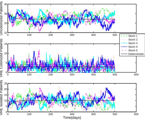
Figure 2: Sample of 5 stochastic realizations in comparison to the numerical solution of the deter-ministic model;N= 37 patients,t𝑠𝑡𝑜𝑝= 500.

Figure 2 depicts a simulation of the stochastic model for a sample of 5 stochastic realizations (𝑁 = 37, 𝑡𝑠𝑡𝑜𝑝 = 500) plotted in comparison to the deterministic numerical solution for the three

compartments. Note that the stochastic realizations exhibit very large differences. However, when carrying out the simulations for larger values ofN, the variation between the stochastic realizations decreases as the value of N increases and are closer to the numerical solution of the deterministic model, as seen in Figure 3. To quantitatively analyze how the variability of the stochastic real-izations decreases as𝑁 increases, we calculated the coefficient of variation (CV) in the range t = [300, 400] using 100 stochastic realizations. These are given in the caption for Figure 3.

3

VRE Surveillance Data

The motivating surveillance data is from an oncology unit, obtained from the VRE Infection Control database of the Department of Quality Improvement Support Service of Yale-New Haven Hospital. Data reports on the number of VRE cases occurred on admission (including patients transferred), the patients’ length of stay, the daily number of patients in isolation due to VRE colonization, the compliance of swab culture administered on admission, and the health care worker contacts precautions compliance. Data collection occurred during the period of January 2005 to January 2007 with a mean number of in-patients per day of 31 patients (with a total of 37 beds).

0 100 200 300 400 500 600 0

20 40 60 80 100 120 140

Time(days)

(a)N=137

0 100 200 300 400 500 600 0

100 200 300 400 500 600

Time(days)

Number of Patients

(b) N=537

0 100 200 300 400 500 600 0

100 200 300 400 500 600 700 800 900 1000

Time(days)

(c)N=937

0 100 200 300 400 500 600 0

500 1000 1500 2000 2500

Time(days)

(d) N=2037

Figure 3: Sample of 5 stochastic realizations for each compartment in comparison to the numerical solution of the deterministic model for N = 137,537,937,2037, t𝑠𝑡𝑜𝑝 = 500. The coefficient of

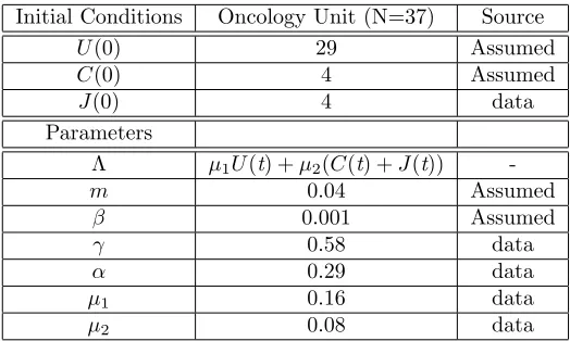
Table 3: Parameters and initial conditions values (some values are assumed for optimization pur-poses)

Initial Conditions Oncology Unit (N=37) Source

𝑈(0) 29 Assumed

𝐶(0) 4 Assumed

𝐽(0) 4 data

Parameters

Λ 𝜇1𝑈(t) +𝜇2(𝐶(t) +𝐽(t))

-𝑚 0.04 Assumed

𝛽 0.001 Assumed

𝛾 0.58 data

𝛼 0.29 data

𝜇1 0.16 data

𝜇2 0.08 data

single room or in a room with another patient who was also VRE positive. If a readmission patient had a positive VRE culture in the past, he/she did not get the rectal swab on admission but was isolated immediately. The isolation report was performed on weekdays (no weekends or holidays). The mean number of isolated VRE colonized patients per day was 9.39 (std=2.90) patients.

3.1 Parameters estimated directly form the surveillance data

Infection control measures were implemented in the form of health care worker hand-hygiene before and after patients contact by the use of gloves and gowns, and washing the hands. For the4 present consideration we are consider the health care worker before patient contact compliance of 57.56% as a better estimator for the parameter 𝛾. In the oncology unit VRE colonized patients had a mean length of stay of 13.15 days (std=18.28) compared with 6.27 (std=6.80) for the uncolonized patients. These means are statistically significantly different supporting the assumption of different discharge rates. Hence, we take 1/𝜇1= 6.27 and 1/𝜇2 = 13.15 giving 𝜇1 = 0.16 and 𝜇2= 0.08.

4

Inverse Problem Methodology

We outline briefly the statistical methodology for estimating parameters in dynamical systems such as (13) using observations of some of the states. More details can be found in [6, 17].

Let 𝑌𝑗 for 𝑗 = 1, ..., 𝑛, be longitudinal data observations (which are random variables)

corre-sponding to the experimental data for the observation process. Since in general 𝑌_𝑗 is not assumed to be free of error (i.e., error in the data collection process), 𝑌𝑗 will not be exactly 𝑓(𝑡𝑗, 𝜃0), the observed part of the true trajectory at time𝑡𝑗. The statistical model that captures the variability

is assumed given by

𝑌𝑗 =𝑓(𝑡𝑗, 𝜃0) +ℰ𝑗 for 𝑗 = 1, .., 𝑛, (14)

in the case of absolute error in the measurements. We can thus envision experimental data as generally consisting of observations from a “perfect” model plus an error component, where 𝜃₀

corresponds to the “true” parameter that generates the observations𝑌𝑗 for𝑗= 1, ..., 𝑛. We assume

that theℰ𝑗’s are generated from a generally unknown probability distribution𝑃. They are assumed

to satisfy the error assumptions

(EA) The random variables ℰ𝑗, 𝑗 = 1...., 𝑛, are independent identically distributed with mean

zero (i.e.,𝐸(ℰ𝑗) = 0) and constant finite variance (i.e., 𝑣𝑎𝑟(ℰ𝑗) =𝜎20 <∞).

The observational process corresponding to the mathematical model (13) is denoted by

𝑓(𝑡𝑗, 𝜃0) =𝐽(𝑡𝑗, 𝜃0). (15)

where the observation function𝑓(𝑡𝑗, 𝜃) depends on the parameters 𝜃 in a nonlinear fashion.

4.1 Ordinary least squares (OLS) estimation

If the error distribution is unknown, an OLS optimization procedure is often employed. This method can be viewed as minimizing the distance between the data and the model where all observations are treated as of equal importance. The OLS method defines “best” as when the norm square of the residuals is a minimum

𝜃𝑂𝐿𝑆 =𝜃𝑂𝐿𝑆𝑛 = arg min𝜃∈Θ 𝑛

∑

𝑗=1

[𝑌𝑗−𝑓(𝑡𝑗, 𝜃)]2. (16)

This corresponds to solving for𝜃 in

𝑛

∑

𝑗=1

[𝑌𝑗−𝑓(𝑡𝑗, 𝜃)]∇𝑓(𝑡𝑗, 𝜃) = 0.

We do not know the distribution of the random variable𝜃𝑂𝐿𝑆, but under asymptotic theory [6, 17,

27] we have as𝑛→ ∞ the approximation

where the covariance matrix Σ𝑛

0 is defined by

Σ𝑛₀ ≡𝜎₀2[𝑛Ω0]−1

with

Ω0≡lim𝑛→∞_𝑛1𝜒𝑛(𝜃0)𝑇𝜒𝑛(𝜃0). Here𝜒𝑛_{(𝜃) ={𝜒}

𝑗𝑘}is the sensitivity matrix given by

𝜒𝑗𝑘(𝜃) = ∂𝑓_∂𝜃(𝑡𝑗, 𝜃)

𝑘 𝑗 = 1, ..., 𝑛 and 𝑘= 1, ..., 𝑝.

The error variance𝜎2

0 is approximated by

ˆ

𝜎_𝑂𝐿𝑆2 = 1

𝑛−𝑝

𝑛

∑

𝑗=1

[𝑦𝑗−𝑓(𝑡𝑗,𝜃ˆ𝑂𝐿𝑆)]2 (18)

as the bias adjusted estimate for𝜎2

0, where ˆ𝜃𝑂𝐿𝑆 is the realization of 𝜃𝑂𝐿𝑆 for a given realization

{𝑦𝑗}of {𝑌𝑗}. The covariance matrix Σ𝑛0 is approximated by ˆ

Σ𝑛_𝑂𝐿𝑆 = ˆ𝜎2_𝑂𝐿𝑆[𝜒𝑇(ˆ𝜃𝑂𝐿𝑆)𝜒(ˆ𝜃𝑂𝐿𝑆)]−1. (19)

Therefore in practice one uses the approximation

𝜃𝑂𝐿𝑆 ∼𝒩𝑝(𝜃0,Σ𝑛0)≈ 𝒩𝑝(ˆ𝜃𝑂𝐿𝑆,Σˆ𝑛𝑂𝐿𝑆). (20)

Asymptotic standard errors for the parameter estimates are obtained by taking square roots of the diagonal elements of ˆΣ𝑛

𝑂𝐿𝑆, i.e., 𝑆𝐸(ˆ𝜃𝑘) =

√

( ˆΣ𝑛

𝑂𝐿𝑆)𝑘𝑘, 𝑘 = 1, ..., 𝑝. The sensitivity matrix

can be calculated by solving the sensitivity equations

𝑑 𝑑𝑡

∂𝑥

∂𝜃 =

∂𝑔 ∂𝑥

∂𝑥

∂𝜃 +

∂𝑔

∂𝜃, (21)

where in our example (13), written as ˙𝑥 =𝑔(𝑥(𝑡), 𝜃), ∂𝑔/∂𝑥 is a 3×3 matrix function and both

∂𝑥/∂𝜃 and ∂𝑔/∂𝜃 are 3×𝑝matrix functions.

4.2 Generalized least squares (GLS) estimation

If the error distribution is unknown and we suspect that relative error is present in the measurement, then the assumption of constant variance of the error in the longitudinal data does not hold. In such cases, a generalized least square (GLS) optimization procedure should be employed. For this case we need to formulate a new statistical model to take into consideration the non-constant error variability. If we can assume that the size of the error depends linearly on the size of the observed quantity, the statistical model (i.e, relative error model) is given by

where the ℰ𝑗 satisfy (EA). It follows that 𝑌𝑗 ∼ 𝒩(𝑓(𝑡𝑗, 𝜃0), 𝜎20𝑓2(𝑡𝑗, 𝜃0)). In this case, GLS can be viewed as minimizing the distance between the data and the model while taking into account a model dependency variance in the observations. The GLS method defines “best” estimator as

𝜃𝐺𝐿𝑆 obtained from solving

𝑛

∑

𝑗=1

𝑓−2(𝑡_𝑗, 𝜃_𝐺𝐿𝑆)[𝑌_𝑗−𝑓(𝑡_𝑗, 𝜃_𝐺𝐿𝑆)]∇𝑓(𝑡_𝑗, 𝜃_𝐺𝐿𝑆) = 0, (23)

with the corresponding estimate ˆ𝜃𝐺𝐿𝑆 for a given realization{𝑦𝑗}. From asymptotic theory [6, 17]

we find

𝜃𝐺𝐿𝑆 =𝜃𝑛𝐺𝐿𝑆 ∼𝒩𝑝(𝜃0,Σ𝑛0) (24)

where

Σ𝑛₀ ≈𝜎₀2[𝜒𝑇(𝜃0)𝑊(𝜃0)𝜒(𝜃0)]−1 with 𝜒(𝜃) = ⎡ ⎢ ⎢ ⎣

∂𝑓(𝑡1,𝜃)

∂𝜃1 ⋅ ⋅ ⋅

∂𝑓(𝑡1,𝜃) ∂𝜃𝑝

..

. ...

∂𝑓(𝑡𝑛,𝜃)

∂𝜃1 ⋅ ⋅ ⋅

∂𝑓(𝑡𝑛,𝜃) ∂𝜃𝑝 ⎤ ⎥ ⎥ ⎦

and 𝑊−1_{(𝜃) = 𝑑𝑖𝑎𝑔(𝑓}2_(𝑡

1, 𝜃), ...,(𝑓2(𝑡𝑛, 𝜃)). Using the estimates we have the covariance matrix

approximation

Σ𝑛₀ ≈Σˆ𝑛_𝐺𝐿𝑆 = ˆ𝜎_𝐺𝐿𝑆2 [𝜒𝑇(ˆ𝜃𝐺𝐿𝑆)𝑊(ˆ𝜃𝐺𝐿𝑆)𝜒(ˆ𝜃𝐺𝐿𝑆)]−1 (25)

and the error variance approximation

ˆ

𝜎2_𝐺𝐿𝑆 = 1

𝑛−𝑝

𝑛

∑

𝑗=1

1

𝑓2_(𝑡

𝑗,𝜃ˆ𝐺𝐿𝑆)

[𝑦𝑗−𝑓(𝑡𝑗,𝜃ˆ𝐺𝐿𝑆)]2. (26)

Therefore in practice we use the approximation

𝜃𝐺𝐿𝑆 ∼𝒩𝑝(𝜃0,Σ𝑛0)≈ 𝒩𝑝(ˆ𝜃𝐺𝐿𝑆,Σˆ𝑛𝐺𝐿𝑆). (27)

We can also calculate the asymptotic standard errors for ˆ𝜃𝐺𝐿𝑆 by taking the square roots of the

diagonal elements of the covariance matrix ˆΣ𝑛

𝐺𝐿𝑆. Again the sensitivity matrix 𝜒(ˆ𝜃𝐺𝐿𝑆) = {𝜒𝑗𝑘}

can be calculated using the sensitivity equations in (21).

Typically, one does not attempt to solve (23) directly, but rather the estimate ˆ𝜃𝐺𝐿𝑆 for a given

realization{𝑦𝑗}can be solved for iteratively using the algorithm:

1. Set𝑘= 0. Estimate the initial ˆ𝜃_𝐺𝐿𝑆(𝑘) by using the OLS estimate with𝑦𝑗 in place of𝑌𝑗 in (16);

2. Form the weights ˆ𝑤𝑘

𝑗 =𝑓−2(𝑡𝑗,𝜃ˆ (𝑘) 𝐺𝐿𝑆);

3. Find ˆ𝜃_𝐺𝐿𝑆(𝑘+1) by minimizing

𝐽𝑘(𝜃𝐺𝐿𝑆) = 𝑛 ∑ 𝑗=1 ˆ 𝑤𝑘

4. Set𝑘=𝑘+ 1 and return to 2. Terminate the process when two successive estimates for ˆ𝜃𝐺𝐿𝑆

are“close” to one another.

4.3 Subset selection algorithm

It is typical that in systems such as (13) some of the parameters (components of 𝜃) are more readily estimated than others. The ability to reliably estimate a parameter is directly related to the sensitivity of the model output to a parameter. In order to identify the subset of parameters that has a high sensitivity to the mathematical model, we use the identifiability analysis recently developed in [14]. The parameter selection or parameter identifiability algorithm consists of considering two criteria:

1. Select the combinations of parameter vectors that have a full rank sensitivity matrix 𝜒𝑛_(ˆ𝜃).

The degree of sensitivity for the matrix is measured in the form of its condition number

𝜅(𝜒𝑛_{(ˆ𝜃)) defined below in (36);}

2. For each parameter vector selected in the first criteria, estimate its degree of uncertainty. Its degree of uncertainty is measured in the form of the parameter selection score 𝜐(ˆ𝜃) defined by (37).

The motivation behind the first criterion is as follows. If 𝜃0 is the true parameter, then Δ𝜃=

𝜃−𝜃₀ denotes a local perturbation from 𝜃₀. This gives rise to a local perturbation Δ𝑦(𝑡) =

𝑦(𝑡, 𝜃)−𝑦(𝑡, 𝜃0) in the output model. Then by a first order Taylor approximation we obtain the approximate relationship

Δ𝑦≈𝜒Δ𝜃. (29)

A parameter vector is identifiable (locally) if the above equation can be solved uniquely for Δ𝜃. This is the case if 𝑟𝑎𝑛𝑘(𝜒) = 𝑝, or equivalently, if and only if the Fisher information matrix,

𝐹 =𝜒𝑇_{(ˆ𝜃)𝜒(ˆ𝜃) is nonsingular or}

det(𝜒𝑇𝜒)∕= 0. (30)

The Fisher information matrix measures the amount of information that an observation process carries about an unknown parameter𝜃. If near-singularity of𝐹is present then the approximation of the covariance matrix and consequently the calculation of standard errors and confidence intervals for the corresponding estimated parameters are affected.

If one focuses on properties of the sensitivity matrix 𝜒(𝜃) rather than the Fisher information matrix, a singular value decomposition (SVD) of the sensitivity matrix plays a crucial role in uncertainty quantification. The SVD of the sensitivity matrix is denoted by

𝜒(𝜃) =𝑈

[

Λ

0 ]

𝑉𝑇 (31)

where 𝑈 = [𝑈₁ 𝑈₂] and 𝑉 are 𝑛×𝑛 and 𝑝×𝑝 orthogonal matrixes, with 𝑈₁ containing the first

𝑝 columns of𝑈 and 𝑈2 containing the last 𝑛−𝑝 columns. Λ is a𝑝×𝑝 diagonal matrix defined as

Λ =𝑑𝑖𝑎𝑔(𝑠1, ..., 𝑠𝑝) with𝑠1 ≥𝑠2≥...≥𝑠𝑝≥0, and0 denotes an (𝑛−𝑝)×𝑝 matrix of zeros.

Suppose that𝑓(𝑡, 𝜃) is well approximated for all𝑡=𝑡𝑗 by its linear Taylor expansion around𝜃0 as

𝑓(𝑡, 𝜃)≈𝑓(𝑡, 𝜃0) +

∂𝑓

Then letting 𝑓(𝜃) = (𝑓(𝑡1, 𝜃), ..., 𝑓(𝑡𝑛, 𝜃))𝑇, 𝑌 = (𝑌1, ..., 𝑌𝑛)𝑇 and ℰ = (ℰ1, ...,ℰ𝑛)𝑇, we have from

(14)

𝑌 −𝑓(𝜃) =−𝜒(𝜃0)(𝜃−𝜃0) +ℰ. (33)

We can then define the estimator𝜃𝑂𝐿𝑆 that minimizes∣𝑌−𝑓(𝜃)∣2and using the invariance property

of the Euclidean norm (i.e.,∣𝑤∣2_=𝑤𝑇_𝑤=𝑤𝑇_{𝐼𝑤=𝑤}𝑇_{𝑈 𝑈}𝑇_𝑤=∣𝑈𝑇_𝑤∣2_{) we have that}

∣𝑌 −𝑓(𝜃)∣2 = ∣ −𝜒(𝜃0)(𝜃−𝜃0) +ℰ∣2

= ¯ ¯ ¯ ¯𝑈𝑇 ( −𝑈 [ Λ 0 ]

𝑉𝑇(𝜃−𝜃0) +ℰ

)¯ ¯ ¯ ¯ 2 = ¯ ¯ ¯ ¯− [ Λ 0 ]

𝑉𝑇(𝜃−𝜃0) +

[ 𝑈𝑇 1 𝑈𝑇 2 ] ℰ ¯ ¯ ¯ ¯ 2 . (34)

Solving ∣ −Λ𝑉𝑇_(𝜃−𝜃

0) +𝑈1𝑇ℰ∣2= 0 for𝜃 we have

𝜃−𝜃0 = (Λ𝑉𝑇)−1𝑈1𝑇ℰ.

This implies

ˆ

𝜃𝑂𝐿𝑆 = 𝜃0+𝑉Λ−1𝑈1𝑇ℰ

= 𝜃0+ 𝑝 ∑ 𝑖=1 1 𝑠𝑖𝑣𝑖𝑢 𝑇

𝑖 ℰ. (35)

Note that if𝑠_𝑖 →0, the estimator is particular sensitive toℰ.

If 𝜒(𝜃) ∈ℝ𝑛×𝑝 _{is a full rank sensitivity matrix (i.e., 𝑟𝑎𝑛𝑘(𝜒(𝜃)) =𝑝) its condition number 𝜅 is}

defined as the ratio of the largest to smallest singular value given by

𝜅(𝜒(𝜃)) = 𝑠1

𝑠_𝑝. (36)

which provides a degree of singularity due to perturbations and hence a criteria for parameter identifiability. If the columns of𝜒(𝜃) are nearly dependent then (36) is large.

Motivation of the second criteria is the uncertainty in the parameters of a particular subset combination that can be quantified using the standard errors 𝑆𝐸(𝜃). In order to compare the degree of variation from one parameter to another, the coefficient of variation 𝐶𝑉 = 𝑆𝐸(𝜃)/𝜃 ∈

ℝ𝑝 _{is used. The 𝐶𝑉 allows one to compare the parameters even if the parameter estimates are}

substantially different in units and scales. Hence, a second criteria can be established by considering the parameterselection score

𝜐(𝜃) =∣𝐶𝑉(𝜃)∣. (37)

In (37) a value near zero indicates lower uncertainty possibilities in the estimation while large values suggest a possibility of a wide uncertainty in at least some of the estimates.

1. Combinatorial search. For a fixed 𝑝, 1 ≤ 𝑝 ≤ 𝐾 (where 𝐾 is total number of parame-ters and initial conditions that are candidates for estimation-for our problem here 𝐾 = 8), calculate the set

𝑆_𝑝={𝜃= (𝑞₁, ..., 𝑞_𝑝)∈ℝ𝑝∣𝑞_𝑘 ∈𝑄_𝐾, 𝑞_𝑘∕=𝑞_𝑙 for all𝑘, 𝑙= 1, ..., 𝑝}

where 𝑄𝐾 = {𝛼, 𝛾, 𝜇1, 𝜇2, 𝐽0, 𝐶0, 𝑚, 𝛽} and the set 𝑆𝑝 collects all the parameter vectors

obtained from the combinatorial search;

2. Full rank test. Calculate the set of feasible parameters Θ𝑝 as

Θ_𝑝 ={𝜃∣𝜃∈𝑆_𝑝 ⊂ℝ𝑝_{, 𝑟𝑎𝑛𝑘(𝜒(𝜃) =𝑝)}. Calculate the condition number defined by}

𝜅(𝜒(𝜃)) = 𝑠1

𝑠_𝑝;

3. Standard error test. For every 𝜃 ∈ Θ𝑝, calculate a vector of coefficients of variation

𝐶𝑉(𝜃)∈ℝ𝑝 _by

𝐶𝑉𝑖=

√

(∑(𝜃)𝑖𝑖

𝜃_𝑖 ,

for𝑖= 1, ..., 𝑝 and ∑(𝜃) =𝜎2

0[𝜒(𝜃)𝑇𝜒(𝜃)]−1 ∈ℝ𝑝×𝑝. Calculate the parameter selection score as𝜐(𝜃) =∣𝐶𝑉(𝜃)∣.

5

Inverse Problem Results

5.1 Optimization algorithm testing with synthetic data

Before illustrating with the VRE surveillance data, we test and illustrate use of the optimization algorithm to investigate the convergence of the parameters estimates ˆ𝜃 to the known values𝜃0. In order to do this, we construct a synthetic dataset{𝑦𝑗} for𝑗= 1, ..., 𝑛, by adding variability to the

corresponding model solution component 𝑓(𝑡𝑗, 𝜃0) = 𝐽(𝑡𝑗, 𝜃0) in (13). The statistical model that captures the variability is taken as

𝑦𝑗 =𝑓(𝑡𝑗, 𝜃0) +𝜎𝑧𝑗 (38)

where𝑧_𝑗 is a realization from a standard normal variable (i.e.,𝑍_𝑗 ∼𝒩(0,1)) and𝜎 is the constant variability. The magnitude of 𝜎 determines how much noise is added. A low value indicates that the data points tend to be very close to the same value (the mean), while high values indicates that the data are “spread out” over a large range of values. Therefore, we can expect that 95% of the time, numbers generated from this distribution will fall in the interval [−1.96𝜎,1.96𝜎]. To this end, we consider the standard error as one indication of the ability of the algorithm to estimate the parameters using the synthetic data set.

The OLS and GLS optimization were solved with MATLAB routine 𝑙𝑠𝑞𝑛𝑜𝑛𝑙𝑖𝑛 for n=500. Parameter upper bounds are taken as

(𝛼, 𝛾, 𝜇1, 𝜇2, 𝐽0, 𝐶0, 𝑚, 𝛽) = (0.5,1,1,1, 𝑁, 𝑁,1,1)

for VRE detection is assumed to take at least 2 days. The model solutions 𝑓(𝑡𝑗, 𝜃0) = 𝐽(𝑡𝑗, 𝜃0) are generated with initial conditions and parameter values𝜃₀ for the oncology unit as described in Table 3 (which are assumed to be the true values). By introducing variability levels such as𝜎 = 0,

𝜎 = 0.01, 𝜎 = 0.05, and 𝜎 = 0.1 in the model solutions the reliability of the algorithm and hence that of estimates are explored. Note that even though we are adding constant variability to the synthetic data, the GLS optimization algorithm is tested with this data. This is because we wish to investigate how the noise affects the standard deviation and not how meaningful they are.

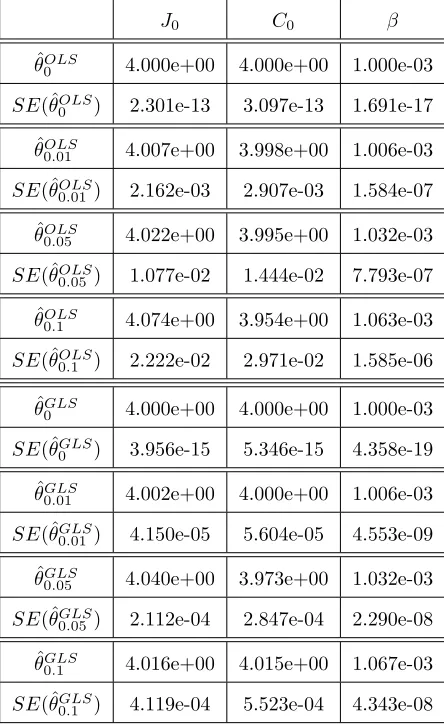
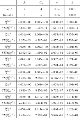
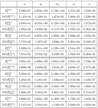
In Tables 4, 5, and 6 we summarize the results for the inverse problems for 𝜃 = (𝐽0, 𝐶0, 𝛽),

𝜃 = (𝐽0, 𝐶0, 𝑚, 𝛽), and 𝜃 = (𝛼, 𝐽0, 𝐶0, 𝑚, 𝛽) using an OLS and a GLS optimization formulation.

Results indicates that both algorithms appear to be reliable for the estimation of the parameters since the estimated values are close to their true values. Note that as𝜎 increases the corresponding standard errors increase. This indicates that the reliability of both algorithms in estimating the parameters may depend on the observational error in the data. Similar results were obtained for the other types of inverse problem formulations.

5.2 Subset selection results using the oncology unit surveillance data

To carry out the subset selection algorithm with the oncology unit surveillance data we assumed nominal parameter values described in Table 3. Since we are interested in estimating the initial conditions, transmission rate, and the fraction of patients that are already colonized on admission, when 𝑝 = 4 the only parameter combination considered is that of 𝜃 = (𝐽0, 𝐶0, 𝑚, 𝛽). When

𝑝= 1,2,3 the only parameters considered are𝜃= (𝛽),𝜃= (𝑚, 𝛽), and𝜃= (𝐽0, 𝐶0, 𝛽).

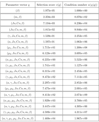
In Table 7 we present the resulting selection score𝜐(𝜃) and condition number𝑘(𝜒(𝜃)) for each subset of parameters when 𝑝 = 1, ...,8. Values that fall in the smallest selection score with the relative small condition number are considered the most feasible subset of parameters. Results in-dicate that the subsets of parameters𝜃= (𝐽0, 𝐶0, 𝑚, 𝛽) have small condition numbers and relatively small selection scores indicating that these subsets might provide low uncertainty in the parameter estimates. In Table 8 we summarize the results of 4 inverse problems corresponding to the subsets with the lowest selection scores and small condition numbers. These subsets of parameters are:

𝜃= (𝛾, 𝐽0, 𝐶0, 𝑚, 𝛽)

𝜃= (𝐽0, 𝐶0, 𝑚, 𝛽)

𝜃= (𝐽0, 𝐶0, 𝛽)

𝜃= (𝑚, 𝛽).

We analyze the results using the coefficient of variation (CV) by considering the effect that the inclusion or exclusion of parameters has on the vector 𝜃 = (𝐽₀, 𝐶₀, 𝑚, 𝛽). In this subset, the standard errors for 𝐽0 is about 0.4% of the estimate, for 𝐶0 it is about 0.8% of the estimate, for

𝑚 it is about 1.6% of the estimate, and for 𝛽 it is 0.3% of the estimate. When including 𝛾 (i.e.,

𝜃 = (𝛾, 𝐽0, 𝐶0, 𝑚, 𝛽)), the CV increases for almost all parameters. On the other hand, when 𝑚

Table 4: OLS and GLS optimization algorithm testing for𝜃= (𝐽0, 𝐶0, 𝛽) using synthetic data. The model was fit to the synthetic data with levels of noise: 𝜎 = 0,0.01,0.05,and 0.1. Subscripts in𝜃_𝜎

denote the level of noise in the synthetic data.

𝐽0 𝐶0 𝛽

ˆ

𝜃𝑂𝐿𝑆

0 4.000e+00 4.000e+00 1.000e-03

𝑆𝐸(ˆ𝜃𝑂𝐿𝑆

0 ) 2.301e-13 3.097e-13 1.691e-17

ˆ

𝜃𝑂𝐿𝑆

0.01 4.007e+00 3.998e+00 1.006e-03

𝑆𝐸(ˆ𝜃𝑂𝐿𝑆

0.01) 2.162e-03 2.907e-03 1.584e-07

ˆ

𝜃𝑂𝐿𝑆

0.05 4.022e+00 3.995e+00 1.032e-03

𝑆𝐸(ˆ𝜃𝑂𝐿𝑆

0.05) 1.077e-02 1.444e-02 7.793e-07

ˆ

𝜃𝑂𝐿𝑆

0.1 4.074e+00 3.954e+00 1.063e-03

𝑆𝐸(ˆ𝜃𝑂𝐿𝑆

0.1 ) 2.222e-02 2.971e-02 1.585e-06

ˆ

𝜃𝐺𝐿𝑆

0 4.000e+00 4.000e+00 1.000e-03

𝑆𝐸(ˆ𝜃𝐺𝐿𝑆

0 ) 3.956e-15 5.346e-15 4.358e-19

ˆ

𝜃𝐺𝐿𝑆

0.01 4.002e+00 4.000e+00 1.006e-03

𝑆𝐸(ˆ𝜃𝐺𝐿𝑆

0.01) 4.150e-05 5.604e-05 4.553e-09

ˆ

𝜃𝐺𝐿𝑆

0.05 4.040e+00 3.973e+00 1.032e-03

𝑆𝐸(ˆ𝜃𝐺𝐿𝑆

0.05) 2.112e-04 2.847e-04 2.290e-08

ˆ

𝜃𝐺𝐿𝑆

0.1 4.016e+00 4.015e+00 1.067e-03

𝑆𝐸(ˆ𝜃𝐺𝐿𝑆

Table 5: OLS and GLS optimization algorithm testing for𝜃= (𝐽0, 𝐶0, 𝑚, 𝛽) using synthetic data. The model was fit to the synthetic data with levels of noise: 𝜎 = 0,0.01,0.05,and 0.1. Subscripts in𝜃_𝜎 denote the level of noise in the synthetic data.

𝐽0 𝐶0 𝑚 𝛽

True𝜃 4 4 0.04 0.001

Initial 𝜃 3 5 0.05 0.002

ˆ

𝜃𝑂𝐿𝑆

0 4.000e+00 4.000e+00 4.000e-02 1.000e-03

𝑆𝐸(ˆ𝜃𝑂𝐿𝑆

0 ) 8.620e-12 1.557e-11 1.611e-13 1.352e-14

ˆ

𝜃𝑂𝐿𝑆

0.01 4.004e+00 4.008e+00 4.013e-02 9.955e-04

𝑆𝐸(ˆ𝜃𝑂𝐿𝑆

0.01) 2.372e-03 4.287e-03 4.457e-05 3.735e-06

ˆ

𝜃𝑂𝐿𝑆

0.05 4.029e+00 3.992e+00 4.032e-02 1.004e-03

𝑆𝐸(ˆ𝜃𝑂𝐿𝑆

0.05) 1.102e-02 1.990e-02 2.091e-04 1.741e-05

ˆ

𝜃𝑂𝐿𝑆

0.1 4.074e+00 3.945e+00 3.987e-02 1.074e-03

𝑆𝐸(ˆ𝜃𝑂𝐿𝑆

0.1 ) 2.271e-02 4.067e-02 4.273e-04 3.529e-05

ˆ

𝜃𝐺𝐿𝑆

0 4.000e+00 4.000e+00 4.000e-02 1.000e-03

𝑆𝐸(ˆ𝜃𝐺𝐿𝑆

0 ) 1.496e-13 2.696e-13 3.145e-15 2.626e-16

ˆ

𝜃𝐺𝐿𝑆

0.01 4.003e+00 4.001e+00 4.003e-02 1.004e-03

𝑆𝐸(ˆ𝜃𝐺𝐿𝑆

0.01) 4.636e-05 8.350e-05 9.762e-07 8.137e-08

ˆ

𝜃𝐺𝐿𝑆

0.05 4.009e+00 4.013e+00 4.022e-02 1.014e-03

𝑆𝐸(ˆ𝜃𝐺𝐿𝑆

0.05) 2.343e-04 4.214e-04 4.971e-06 4.118e-07

ˆ

𝜃𝐺𝐿𝑆

0.1 4.050e+00 4.011e+00 4.046e-02 1.025e-03

𝑆𝐸(ˆ𝜃𝐺𝐿𝑆

Table 6: OLS and GLS optimization algorithm testing for𝜃= (𝛼, 𝐽0, 𝐶0, 𝑚, 𝛽) using synthetic data. The model was fit to the synthetic data with levels of noise: 𝜎 = 0,0.01,0.05,and 0.1. Subscripts in𝜃𝜎 denote the level of noise in the synthetic data.

𝛼 𝐽0 𝐶0 𝑚 𝛽

ˆ

𝜃𝑂𝐿𝑆

0 2.890e-01 4.003e+00 4.136e+00 4.451e-02 1.856e-03

𝑆𝐸(ˆ𝜃𝑂𝐿𝑆

0 ) 2.145e-04 5.126e-04 1.674e-03 2.009e-05 1.220e-06

ˆ

𝜃𝑂𝐿𝑆

0.01 2.895e-01 4.010e+00 4.120e+00 4.454e-02 1.872e-03

𝑆𝐸(ˆ𝜃𝑂𝐿𝑆

0.01 ) 1.094e-03 2.620e-03 8.517e-03 1.025e-04 6.264e-06

ˆ

𝜃𝑂𝐿𝑆

0.05 2.811e-01 4.023e+00 4.269e+00 5.080e-02 1.670e-03

𝑆𝐸(ˆ𝜃𝑂𝐿𝑆

0.05 ) 5.755e-03 1.337e-02 4.696e-02 6.381e-04 3.168e-05

ˆ

𝜃𝑂𝐿𝑆

0.1 2.899e-01 4.051e+00 4.109e+00 4.541e-02 1.880e-03

𝑆𝐸(ˆ𝜃𝑂𝐿𝑆

0.1 ) 1.071e-02 2.572e-02 8.329e-02 1.033e-03 6.263e-05

ˆ

𝜃𝐺𝐿𝑆

0 2.901e-01 4.000e+00 4.095e+00 4.325e-02 1.538e-03

𝑆𝐸(ˆ𝜃𝐺𝐿𝑆

0 ) 3.606e-06 8.920e-06 2.854e-05 3.686e-07 2.277e-08

ˆ

𝜃𝐺𝐿𝑆

0.01 2.894e-01 4.009e+00 4.130e+00 4.300e-02 1.869e-03

𝑆𝐸(ˆ𝜃𝐺𝐿𝑆

0.01) 2.282e-05 5.581e-05 1.836e-04 2.373e-06 1.525e-07

ˆ

𝜃𝐺𝐿𝑆

0.05 2.787e-01 4.030e+00 4.348e+00 2.360e-02 1.860e-03

𝑆𝐸(ˆ𝜃𝐺𝐿𝑆

0.05) 1.068e-04 2.581e-04 8.901e-04 5.955e-06 5.713e-07

ˆ

𝜃𝐺𝐿𝑆

0.1 2.900e-01 4.035e+00 4.189e+00 4.739e-02 1.882e-03

𝑆𝐸(ˆ𝜃𝐺𝐿𝑆

Table 7: Subset parameter selected as a result of the selection algorithm for𝑝 = 1, ...,8 using the oncology unit surveillance data with nominal parameter values described in Table 3 using the GLS optimization.

Parameter vector𝑞 Selection score𝜐(𝑞) Condition number 𝜅(𝜒(𝑞))

(𝛽) 1.975e-05 1.000e+00

(𝑚, 𝛽) 2.358e-03 8.070e+02

(𝐽𝑜, 𝐶𝑜, 𝛽) 7.134e-03 8.236e+04

(𝐽𝑜, 𝐶𝑜, 𝑚, 𝛽) 1.815e-02 9.946e+04

(𝛾, 𝐽𝑜, 𝐶𝑜, 𝑚, 𝛽) 1.539e-01 2.253e+05

(𝛼, 𝐽𝑜, 𝐶𝑜, 𝑚, 𝛽) 1.597e-01 1.063e+06

(𝜇1, 𝐽𝑜, 𝐶𝑜, 𝑚, 𝛽) 1.715e+01 1.308e+08

(𝜇2, 𝐽𝑜, 𝐶𝑜, 𝑚, 𝛽) 6.123e+03 3.695e+05

(𝛼, 𝜇1, 𝐽𝑜, 𝐶𝑜, 𝑚, 𝛽) 6.225e+00 5.522e+06

(𝛾, 𝜇1, 𝐽𝑜, 𝐶𝑜, 𝑚, 𝛽) 1.741e+01 1.127e+08

(𝛼, 𝜇2, 𝐽𝑜, 𝐶𝑜, 𝑚, 𝛽) 6.315e+01 2.453e+05

(𝛾, 𝜇2, 𝐽𝑜, 𝐶𝑜, 𝑚, 𝛽) 8.472e+02 7.112e+05

(𝛼, 𝛾, 𝐽𝑜, 𝐶𝑜, 𝑚, 𝛽) 2.297e+03 2.852e+06

(𝜇1, 𝜇2, 𝐽𝑜, 𝐶𝑜, 𝑚, 𝛽) 7.475e+04 2.091e+05

(𝛼, 𝛾, 𝜇1, 𝐽𝑜, 𝐶𝑜, 𝑚, 𝛽) 8.413e+02 2.074e+09

(𝛼, 𝜇1, 𝜇2, 𝐽𝑜, 𝐶𝑜, 𝑚, 𝛽) 1.929e+03 3.760e+05

(𝛼, 𝛾, 𝜇2, 𝐽𝑜, 𝐶𝑜, 𝑚, 𝛽) 3.447e+04 4.305e+06

(𝛾, 𝜇1, 𝜇2, 𝐽𝑜, 𝐶𝑜, 𝑚, 𝛽) 4.589e+04 4.311e+07

Table 8: Results of 4 inverse formulations solved with nominal values in Table 3 via GLS optimiza-tion for the oncology unit surveillance data.

𝛾 𝐽0 𝐶0 𝑚 𝛽

ˆ

𝜃 6.392e-01 4.004e+00 1.092e+00 5.277e-02 4.770e-03

𝑆𝐸(ˆ𝜃) 2.680e-02 1.811e-02 4.985e-02 6.007e-03 3.955e-04

𝐶𝑉(ˆ𝜃) 4.192e-02 4.524e-03 4.567e-02 1.139e-01 8.291e-02

ˆ

𝜃 - 3.706e+00 1.966e+00 3.608e-02 4.865e-03

𝑆𝐸(ˆ𝜃) - 1.499e-02 1.560e-02 5.616e-04 1.675e-05

𝐶𝑉(ˆ𝜃) - 4.044e-03 7.934e-03 1.556e-02 3.443e-03

ˆ

𝜃 - 3.706e+00 1.966e+00 - 4.865e-03

𝑆𝐸(ˆ𝜃) - 1.419e-02 1.184e-02 - 9.945e-08

𝐶𝑉(ˆ𝜃) - 3.829e-03 6.020e-03 - 2.044e-05

ˆ

𝜃 - - - 4.070e-02 4.725e-03

𝑆𝐸(ˆ𝜃) - - - 9.290e-05 2.802e-06

𝐶𝑉(ˆ𝜃) - - - 2.282e-03 5.931e-04

0 100 200 300 400 500 −8

−6 −4 −2 0 2 4 6 8 10

(a) OLS: Residuals vs Time

3 4 5 6 7 8 9 10 −8

−6 −4 −2 0 2 4 6 8 10

(b) OLS: Residuals vs Model

0 100 200 300 400 500 −0.8

−0.6 −0.4 −0.2 0 0.2 0.4 0.6 0.8 1

(c) GLS: Residuals/Model vs Time

3 4 5 6 7 8 9 10 −0.8

−0.6 −0.4 −0.2 0 0.2 0.4 0.6 0.8 1

(d) GLS: Residuals/Model vs Model

0 50 100 150 200 250 300 350 400 450 500 2

4 6 8 10 12 14 16 18 20

Time (days)

VRE Colonized Patients in Isolation

Figure 5: Best fit model solutions to oncology unit surveillance data via GLS optimization, ( ˆ𝐽0,𝐶ˆ0,𝜇ˆ2,𝛽ˆ) = (4,2,0.04,0.0049).

6

Concluding Remarks

Over the past decade efforts to connect models to data in the context of disease dynamics have grown dramatically albeit most of the efforts have been carried out in the context of deterministic epidemic models [13]. However, not only is it the case that the use of stochastic Markov Chain models is often most appropriate, but also the use of stochastic processes in epidemiology has had a long and distinguished history going back to 1766 [18].

7

Acknowledgments

This research was supported in part by the Alfred P. Sloan Foundation Graduate Scholarship (sponsored by the Sloan Foundation and NACME), the Louis Stokes Alliance for Minority Par-ticipation (LSAMP) Fellowship (sponsored by NSF/WAESO), and the More Graduate Education at Mountain State Alliance (MGE@MSA) Scholarship. It was also supported in part by the U.S. Air Force Office of Scientific Research under grant AFOSR-FA9550-09-1-0226 and in part by the National Institute of Allergy and Infectious Disease under grant NIAID 9R01AI071915-05. The authors are grateful to Dr. Carlos Torres-Viera for providing the sample data used to illustrate the methodology.

References

[1] L. Allen, An Introduction to Stochastic Processes with Applications to Biology, Pearson Education-Prentice Hall, New Jersey, 2003.

[2] D. J . Austin, M. J . M. Bonten, R. A. Weinstein, S. Slaughter, and R. M. Anderson, Vancomycin-resistant enterococci in intensive-care hospital settings: transmission dynamics, persistence, and the impact of infection control programs, Proc. Natl. Acad. Sci. USA, 96

(1999), 6908–6913.

[3] D. J . Austin, and R. M. Anderson, Transmission dynamic of epidemic methicillin-resistant staphylococcus aureus and vancomycin-resistant enterococci in England and Wales, The Jour-nal of Infectious Diseases, 179(1999), 883–891.

[4] D. J . Austin, M. Kakehashi, and R. M. Anderson, The transmission dynamic of antibiotic-resistant bacteria: the relationship between resistance in commensal organisms and antibiotic consumption,Proc. Biol. Sci., 264(1997), 1629–1638.

[5] P. Bai, H. T. Banks, S. Dediu, A. Y. Govan, M. Last, A. Lloyd, H. K. Nguyen, M. S. Olufsen, G. Rempala, and B. D. Slenning, Stochastic and deterministic models for agricultural production networks, Mathematical Biosciences and Engineering,4 (2007), 373–402.

[6] H. T. Banks, M. Davidian, J.R. Samuels Jr., and K. L. Sutton, An inverse problem statisti-cal methodology summary, Center for Research in Scientic Computatione Technistatisti-cal Report, CRSC-TR08-01, 2008, North Carolina State University; inMathematical Statistical Estimation Approaches in Epidemiology, G. Chowell et al. (eds), Springer, New York, 2009, 249–302. [7] M. J. M. Bonten, R. Willems, and R. A. Weinstein, Vancomycin-Resistant Enterococci: why

are they here, and where do they come from?, The Lancet Infectious Diseases, 1(5) (2001), 314–325.

[8] F. Brauer and C. Castillo-Chavez, Mathematical Models in Population Biology and Epidemi-ology, Texts in Applied Mathematics, Volume 40, Springer-Verlag, New York, 2001.

[10] K. E. Byers, A. M. Anglim, C. J. Anneski, and B. M. Farr, Duration of colonization with vancomycin-resistant enterococcus, Infection Control and Hospital Epidemiology, 27 (2002), 271–278.

[11] C. Castillo-Chavez, K. C. Chow, and X. Wang, A mathematical model of nosocomial infection and antibiotic resistance: evaluating the efficacy of antimicrobial cycling programs and patient isolation on dual resistance, Mathematical and Theoretical Biology Institute Technical Reports, MTBI-04-05M, Arizonia State University, 2007.

[12] G. Chowell, P. W. Fenimore, M. A. Castillo-Garsow, and C. Castillo-Chavez, SARS outbreaks in Ontario, Hong Kong and Singapore: the role of diagnosis and isolation as a control mecha-nism, J. Theor. Biol.,224(2003), 1–8.

[13] G. Chowell, J.M. Hyman, L.M.A. Bettencourt, and C. Castillo-Chavez (Eds), Mathematical and Statistical Estimation Approaches in Epidemiology, Springer, New York, 2009.

[14] A. Cintron-Arias, H.T. Banks, A. Capaldi, and A.L. Lloyd, A sensitivity matrix based method-ology for inverse problem formulation,J. of Inverse and Ill-posed Problems,15(2009), 545–564. [15] B. S. Cooper, G. F. Medley, and G. M. Scott, Preliminary analysis of the transmission dynamics of nosocomial infections: stochastic and management effects, J. of Hospital Infection, 43

(1999), 131–147.

[16] E. M. C. D’ Agata , M. A. Horn, and G. F. Webb, The impact of persistent gastrointestinal colonization on the transmission dynamics of vancomycin-resitant enterococci, The Journal of Infectious Diseases,185 (2002), 766–773.

[17] M. Davidian and D. M. Giltinan, Nonlinear models for Repeated Measurement Data, Mono-graphs on Statistics and Applied Probability, Vol. 62. Chapman and Hall/CRC Press, Boca Raton, FL, 1995.

[18] Klaus Dietz and J.A.P. Heesterbeek, Daniel Bernoullis epidemiological model revisited,Math. Biosci., 180 (2002) 1-21.

[19] S. N. Ethier and T. G. Kurtz,Markov Processes: Characterization and Convergence, J. Wiley and Sons, New York, 1986.

[20] D. T. Gillespie, A General method for numerically simulating the stochastic time evolution of coupled chemical reactions, J. Computational Physics,22(1976), 403–434.

[21] B. Grenfell and A. Dobson,Ecology of Infectious Diseases in Natural Populations, Cambridge University Press, Cambridge, 1995.

[22] T.G. Kurtz, Solutions of ordinary differential equations as limits of pure jump Markov pro-cesses, J. Applied Probability,7 (1970), 49–58.

[24] M. A. Montecalvo, W. R. Jarvis, J. Uman, D. K. Shay, C. Petrullo, K. Rodney, C. Gedris, H. W. Horowitz, and G. P. Wormser, Infection-control measures reduce transmission of vancomycin-resistant enterococci in an endemic setting,Annals of Internal Medicine,131(1999), 269–272. [25] A. R. Ortiz, H. T. Banks, C. Castillo-Chavez, G. Chowell, C. Torres-Viera, and X. Wang, Mod-eling the transmission of Vancomycin-resistant enterococcus (VRE) in hospitals: a case study, Center for Research in Scientic Computation Technical Report, CRSC-TR10-05, February, 2010, North Carolina State University, Raleigh.

[26] E. Renshaw,Modeling Biological Populations in Space and Time, Cambridge Studies in Math-ematical Biology (No. 11), Cambridge, 1991.

[27] G. A. F. Seber and C. J. Wild,Nonlinear Regression, John Wiley & Sons, New York, 1989. [28] J. Y. Song, H. J. Cheong, Y. M. Jo, W. S. Choi, J. Y. Noh, J. Y. Heo, W. J. Kim,

Vancomycin-resistant Enterococcus colonization before admission to the intensive care unit: A clinico-epidemiologic analysis,American Journal of Infection Control,37 (2009), 734–740.