Abstract
Bao, Shengli. A Comparison of Two Algorithms for Clearing Multi-unit Bid Double Auctions. (Under the direction of Peter R. Wurman)
A COMPARISON OF TWO ALGORITHMS FOR
CLEARING MULTI-UNIT BID DOUBLE AUCTIONS
BY SHENGLI BAO
DEPARTMENT OF COMPUTER SCIENCE NORTH CAROLINA STATE UNIVERSITY
DECEMBER 1, 2002
A THESIS SUBMITTED TO THE GRAUDTAE FACULTY OF NORTH CAROLINA STATE UNIVERSITY
IN PARTIAL FULFILMENT OF THE RQUIREMENT FOR THE DEGREE OF MASTER OF SCIENCE
APPROVED BY
_________________________ PETER WURMAN
CHAIR OF ADVISORY COMMITTEE
__________________________ MUNINDAR P. SINGH
Biography
I was born in Luoyang, China, a beautiful city famous for its peony flowers, grottoes, and ancient history. After graduated from high school, I went to study at Zhengzhou University. I worked about three years in China and came to America to further my education in 1998. Grateful for the American Education Systems, I was free to study any subject I had interested in. I got one BS degree in Computer Science, one MBA degree concentrated on Finance and one MS degree in Computer Science during these five years of study.
Acknowledgement
I’d like to thank Dr. Peter R. Wurman for his guidance and advice. I am very glad to have him as my teacher and advisor.
I thank Dr. Singh and Dr. Chirkova for being on my thesis committee.
I thank my family for their love and support.
Table of Contents
List of Tables vi
List of Figures vii
1. Introduction 1
2. Formal Problem Specifications 2
2.1. The Mth and (M+1) st Prices 2
2.2. The Transaction Set 3
2.3. The Four Auction Actions 4
2.4. The Bid Priority Rules 4
3. The Multi-unit Bid 4-Heap Algorithm 5
3.1. The Four Heaps 6
3.2. The Mth and (M+1) st Prices in a Single Unit Bid Double Auction 7 3.3. The Mth and (M+1) st Prices in a Multi-unit Bid Double Auction 7
3.4. The 4-Heap Insert Action 8
3.4.1. Examples for the Insert Action 8
3.4.2. Inserting a New Bid into Bin 10
3.4.3. Inserting a New Bid into Sin 12
3.4.4. Insert Action Algorithm 13
3.4.5. The Complexity Analysis of the 4-Heap Insert Action 13
3.5. The 4-Heap Price Quote Action 14
3.6. The 4-Heap Withdraw Action 15
3.7. The 4-Heap Clear Action 15
3.8. The Worst Case Complexity Analysis of the Four Auction Actions 16
4. The Multi-unit Bid IPR Tree Algorithm 16
4.1. The IPR Tree 17
4.2. Different Balanced Trees 19
4.3. The IPR Tree Insert Action 20
4.3.1. The Next Higher Priority Node of the Node T 21
4.3.2. Examples for Finding the Next Higher Priority Node 21
4.3.3. The Algorithm for Finding the Next Higher Priority Node 24
4.3.4. The Previous Lower Priority Node of the Node T 25
4.3.5. Move-up-q-units 25
4.3.6. Unit Counter 27
4.3.7. Move-up-q-units 29
4.3.8. Move-down-q-units 29
4.3.9. The IPR Tree Insert Action Algorithm 30
4.4. The IPR Tree Price Quote Action 32
4.5. The IPR Tree Withdraw Action 32
4.6. The IPR Tree Clear Action 33
4.7. The Worst Case Complexity Analysis of the Four Auction Actions 35
5. Experimental Evaluation of the Two Algorithms 35
5.1. The Impact of the Number of Bids on Algorithm Performance 36
5.2. The Impact of Bid Quantity on Algorithm Performance 37
5.3. The Impact of the Clear Action on Algorithm Performance 39
5.4. The Impact of Bid Ordering on Algorithm Performance 40
6. Conclusions 43
7. References 44
List of Tables
3.1 The worst case complexity analysis of the 4-Heap insert action 14
3.2 The worst case complexity analysis of the 4-Heap withdraw action 15
3.3 The worst case complexity analysis of the four auctions actions in the 4-Heap
algorithm 16
4.1 The complexity analysis for different tree structures in insert, look-up and
withdraw operations 19
4.2 The worst case complexity analysis for an AVL and an IPR tree 19
4.3 The worst case complexity analysis of the four auction actions in the IPR tree
algorithm 35
5.1 The actual CPU time with different number of bids 36
5.2 The actual CPU time with different bid quantity 37
5.3 The actual CPU time for different clear intervals 39
5.4 The percentage of clear action CPU time 39
5.5 The actual CPU time for different bid distributions 41
List of Figures
2.1 The Mth and (M+1) st prices in a multi-unit bid auction 3
3.1 The four heaps in the 4-Heap algorithm 6
3.2 The original 4 heaps before inserting a new buy bid 8
3.3 The new 4 heaps after inserting a new buy bid 9
3.4 The general case for inserting a new buy bid into Bin 10
3.5 The general case for inserting a sell bid into Sin 12
4.1 The four balance rotations in the IPR tree 17
4.2 The next higher priority node ---example 1 21
4.3 The next higher priority node ----example 2 22
4.4 The next higher priority node ----example 3 23
4.5 Move-up-q-units example 26
4.6 The unit counters in an IPR tree 28
4.7 Withdrawing a node from an IPR tree 32
5.1 The impact of number of bids on algorithm performance 36
5.2 The exponential distribution 38
5.3 The diverge and converge of bid distributions 40
5.4 The different bid converge and diverge distributions 41
1. Introduction
In auctions, potential buyers and sellers submit bids for specific goods or services. Automated negotiations help to decide which buyers get which sellers’ goods or services and at which price. In this paper, two algorithms for managing bids in an auction are examined: the 4-Heap algorithm [1] and the IPR tree algorithm. These two algorithms are constructed for auctions with multiple buyers and sellers that do not clear instantaneously. They form price formation mechanisms to determine market clearing prices.
The 4-Heap algorithm is introduced by Wurman, Walsh, and Wellman [1]. This algorithm uses four heap structures to organize the bids, and the discussion of the 4-Heap algorithm is based on single unit bids. Here we extend their theory to include multi-unit bids.
In addition, I introduce an IPR tree algorithm for multi-unit bids. This algorithm exhibits improved efficiency for processing bids and calculating allocations under certain scenarios. A runtime comparison analysis of the two algorithms is presented, which points out each algorithm’s advantages and disadvantages.
Motivation
There are numerous applications of double auctions in electronic commerce, including stock exchanges, B2B commerce, and bandwidth allocation. However, not that much has been published on algorithms. This is our main motivation to implement and later examine the 4-Heap and the IPR tree algorithms.
What research has been done for double auction algorithms primarily considers single unit bids. In our algorithms, we allow multi-unit bids, though we require bids to be divisible.
The Mth and (M+1) st price rules are well known in the double auction theory and applications. They define the range of equilibrium prices, which balance the market demand and supply. In our algorithms, we examine how to keep track of the Mth and (M+1) st prices incrementally while processing the multi-unit bids.
Thesis Organization
Section 2 presents background concepts about double auctions, including the Mth and (M+1) st price rules, the four auction actions, and the bid tie-breaking rules. Section 3 explains the Multi-unit Bid 4-Heap Algorithm. It organizes the discussion of the algorithm around the four auction actions, and presents the complexity analysis for each action. Section 4 presents the Multi-unit Bid IPR Tree Algorithm. It also breaks down the algorithm according to the four auction actions and analyzes these actions’ performance complexity. Section 5 compares these two algorithms’ performance under different experiments. Section 6 concludes with each algorithm’s advantages and disadvantages.
2. Formal Problem Specification
2.1. The Mth and (M+1) st Prices
The Mth and (M+1) st prices determine the range of equilibrium prices and which bids are winning bids. Consider l single unit bids, of which m are sell bids, and the remaining n= l-m are buy bids. Single unit bids refer to the bids whose quantities are restricted to be one. Sorting the buy and sell bids in decreasing order by price, the Mth price is the mth highest bid among all bids, and the (M+1) st price is the (m+1) st highest bid among all bids. The Mth and (M+1) st prices are necessarily set by different bids, though they may still have the same price.
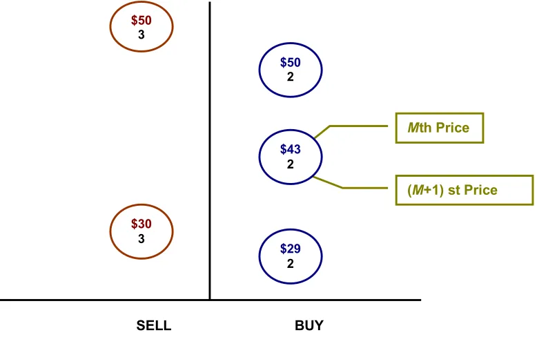
For multi-unit, divisible bids, let q denote the total number of units offered in the m sell bids. Multi-unit bids refer to the bids whose quantities can be more than one. Again sort the buy and sell bids in decreasing order by price. The Mth price is the price of the qth unit. And the (M+1) st price is the price of (q+1) st unit. The Mth and (M+1) st prices may be set by the same bid or by different bids.
Figure 2.1. The Mth and (M+1) st prices in a multi-unit bid auction.
An example is shown in Figure 2.1. There are 2 sell bids and 3 buy bids. Each sell bid has 3 units. Each buy bid has 2 units. Sort the bids in decreasing order by price. The Mth price is the price of the 6th unit. The (M+1) st price is the price of the 7th unit. The Mth
and (M+1) st prices happen to be in the same buy bid.
2.2. The Transaction Set
Let s denote the number of sell units at or below the clearing price, and b the number of buy units at or above the clearing price. A transaction set consists of the b highest buy units and s lowest sell units under the condition that b is equal to s. When a uniform
$50 3
BUY SELL
Mth Price
(M+1) st Price
$30 3
$50
2
$43
2
$29
2
clearing price is selected, the buy and sell bids in the transaction set can be arbitrarily matched successfully.
In Figure 2.1, the transaction set includes all the buy units above $43 and 1 unit whose price is $43, and all the sell units below $43. Therefore this transaction set has 3 buy units and 3 sell units.
2.3 The Four Auction Actions
A bid management algorithm in a multi-unit bid double auction has to support four actions. The four actions are:
1. Insert:
Inserts a new bid into the bid data structure, and updates the Mth and (M+1) st prices. 2. Price Quote:
Generates the Mth and (M+1) st prices. 3. Withdraw:
Removes an active bid from the bid data structure, and updates the Mth and (M+1) st prices.
4. Clear:
Removes all the bids in the transaction set according to one clearing price.
In our analysis of the 4-Heap and IPR tree algorithms, we examine these two algorithms’ methods and efficiency in handling each action.
2.4 The Bid Priority Rules
In order to get the Mth and (M+1) st prices, we need a total order on bids. The bid priority rules determine the sorted order of bids, and compare bids based on the bid price, bid type and bid ID. Let p denote the bid price, t denote the bid type, and ID denote the bid ID. These rules for comparing bid i with bid j are:
If pi> pj, then i > j.
Else if pi < pj, then i< j.
Else
If ti = buy & tj = sell, then i> j.
Else if ti = sell& tj = buy, then i< j.
Else if IDi > IDj, then i> j.
Else i< j.
Since bid IDs are always unique for the auctioneers, there are no equal bids existed in the bid data structure. In practice, auctions often use time as the final tiebreaker, giving preference to the bids that arrive earlier.
3. The Multi-unit Bid 4-Heap Algorithm
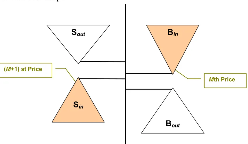
One algorithm proposed to manage bids is the 4-Heap algorithm [1]. It involves two max-heaps and two min-max-heaps [Figure 3.1]. A max-heap refers to a heap structure whose root holds the biggest value. A min-heap refers to a heap structure whose root holds the smallest value. These four heaps are constructed in a manner that is consistent with the Mth and (M+1) st prices.
3.1. The Four Heaps
Figure 3.1. The four heaps in the 4-Heap algorithm.
Bin:
Bin holds all the buy units whose prices are greater than or equal to the Mth price.1
Bin is implemented as a min-heap with the lowest price bid at the root.
Bout:
Bout holds all the buy units whose prices are less than or equal to the Mth price.1
Bout is implemented as a max-heap with the biggest price bid at the root.
Sin:
Sin holds all sell units whose prices are smaller than or equal to the (M+1) st
price.1 S
in is implemented as a max-heap with the highest price bid at the root.
Sout:
Sout holds all the sell units whose prices are greater than or equal to the (M+1) st
price. 1 Sout is implemented as a min-heap with the smallest price bid at the root.
1 If the Mth and (M+1) st prices are equal, neither buyers nor sellers with offers at that price can determine whether they are wining or losing [1].
B
inS
inS
outB
outMth Price
(M+1) st Price
The 4-Heap algorithm enforces several constraints. Let pr denote the bid priority and u denote the number of units in each heap. The followings are the constraints:
u (Bin) = u (Sin)
pr(Bin) ≥ pr(Bout)
pr(Sout) ≥ pr(Sin)
pr(Bin) > pr(Sin)
pr(Sout) > pr(Bout)
Equal priority may happen when the same buy bid is subdivided and put into Bin and Bout
or the same sell bid is subdivided between Sin andSout.
3.2. The Mth and (M+1) st Prices in a Single Unit Bid Double Auction
In a single unit bid double auction, the Mth and (M+1) st prices are necessarily set by different bids, though they may still have the same price. The Mth price is the price of the smallest bid among Sout and Bin. And the (M+1) st price is the price of the largest bid
among Sin and Bout. Sin and Bin form the transaction set and can be cleared at the clearing
price.
3.3. The Mth and (M+1) st Prices in a Multi-unit Bid Double Auction
For multi-unit bids, bid price, bid type and bid quantity determine the Mth and (M+1) st prices. A single unit bid double auction is a special case of a multi-unit bid double auction, where all the bids’ quantities are restricted to be one.
Contrary to a single unit bid double auction, where the Mth and (M+1) st prices must be set by different bids, in a multi-unit bid double auction the Mth and (M+1) st prices may be set by different bids or by the same bid. This poses a slight problem for the 4-Heap algorithm that can be overcome by subdividing some bids into two different bids.2 If a
buy bid sets both the Mth and (M+1) st prices, it is divided between Bin and Bout. If a sell
bid sets both the Mth and (M+1) st prices, it is divided between Sin and Sout.
3.4. The 4-Heap Insert Action
When inserting one multi-unit bid using the 4-Heap algorithm, bid price, bid type and bid quantity determine which heap this new bid belongs to. Different bid types cause different bid movements. When inserting a new buy bid into Bin, the direction of the bid
movements is downward from Bin to Bout or from Sout to Sin. When inserting a new sell
bid into Sin, the direction of the bid movement is upward from Sin to Sout or Bout to Bin.
3.4.1. Examples for the Insert Action
Figure 3.2. The original 4 heaps before inserting a new buy bid.
According to the auction data in Figure 2.1, we build the four heaps in Figure 3.2. There are altogether 6 sell units. The Mth price is $43, which is the price of the 6th highest unit when the bids are sorted according to the bid priority rules. The (M+1) st price is $43, which is the price of the 7th highest unit.
New Bid
$30 3
(M+1) st Price
Mth Price
$50 3
$50
2
$43
1
$43
1
$29
2
$50 3
The bid whose price is $43 is subdivided into two bids. One bid is in Bin and becomes the
Mth price bid. The other is in Bout and becomes the (M+1) st price bid. The transaction set
has 3 units. Bin has all the buy units whose prices are above $43 and the Mth price bid. Sin
has all the sell units whose prices are below $43.
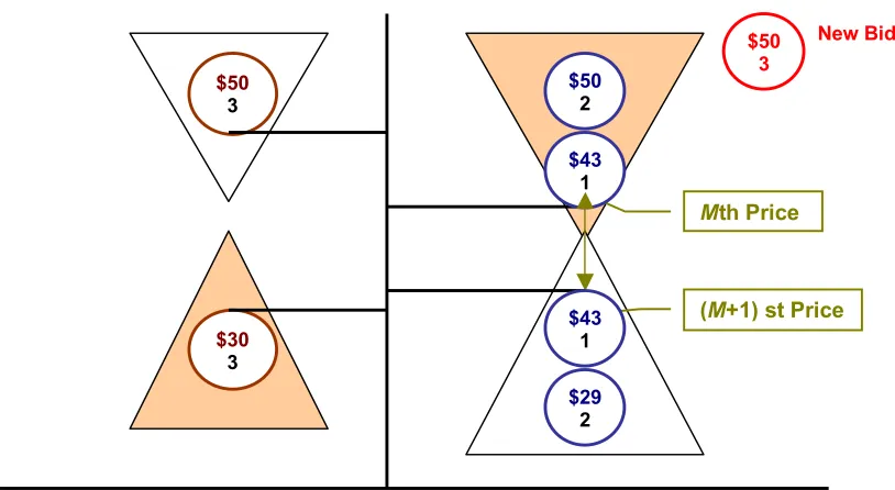
Figure 3.3. The new 4 heaps after inserting a new buy bid.
In Figure 3.3 a new bid to buy 3 units at $50 is inserted. After inserting this new buy bid that has higher priority than the Mth price bid, the Mth and (M+1) st prices are moved upward by the new bid quantity. The Mth price is moved upward by 3. Now the Mth price unit is the first unit in the sell bid with price at $50. The (M+1) st price is also moved upward by 3 and is the second unit in the sell bid with price at $50.
Several bids have to be moved to retain the 4-heap consistency. First move the $43 buy bid down from Bin to Bout. The reason to move is due to this bid is smaller than the new
Mth price bid, and it can not be kept in the Bin. The Bin now has 5 buy units. Subdivide
the sell bid with price at $50 into two connected sell bids. 2 units move downward from Sout to Sin. The remaining one unit is kept in Sout. After these bid movements, the Mth
price is $50, and the (M+1) st price is also $50. The transaction set now has 5 units.
Mth Price
(M+1) st Price
$50 3
$29
2 $30
3 $50
1
$50
2
$50 2
1 2
$43
2
Complicated bid movements take place when inserting a new buy bid into Bin or inserting
a new sell bid into Sin. Multiple lg (n) operations happen under these two situations.
Figure 3.4 and Figure 3.5 generalize the bid movements when inserting a new bid into Bin
or Sin.
3.4.2.Inserting a New Bid into Bin
This situation takes place when we insert a new buy bid and this bid has higher priority than the current Mth price bid.
When we push a bid into a heap or pop a bid from a heap, in order to maintain the heap structure, we move either the highest priority bid or the lowest priority bid to the root of the heap depending on whether the heap is a max-heap or a min-heap. This operation takes lg (n) time.
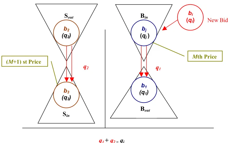
Figure 3.4. The general case for inserting a new buy bid into Bin.
q1+ q2= qi
New Bid
Bout
Sout
Sin
q1 q2
Bin
Mth Price (M+1) st Price
bj
(qj )
bi
(qi)
b2
(q2)
b3
(q3)
b1
(q1)
Figure 3.4 shows the downward bid movements when inserting a new buy bid into Bin. q1
denotes the number of units moved from Bin to Bout; q2 denotes the number of units
moved from Sout to Sin. qiis the new buy bid quantity, which is equal to the sum of q1and
q2.
Let b denote bid, bidenote the new bid, bjdenote the minimum bid among Sout and Bin, q
denote bid quantity,
1. If qi = = qj, 3 lg (n) operations take place.
a. Push bi into Bin.
b. Pop bj from Bin or Sout.
c. Push bj into Bout or Sin.
2. If qi < qj, 2lg (n) operations take place.
a. Push bi into Bin.
b. Subdivide bj according to qi. Keep qi units in Bin or Sin, and push qj - qi
units into Bout or Sout.
3. If qi > qj, multiple lg (n) operations happen. In the worst case, (2q+1)lg (n)
operations take place. a. Push bi into Bin.
b. Repeat if qi ≤ qj. In the worst case, q times are repeated.
i. Pop bj from Bin or Sout.
ii. Push bj into Bout or Sin.
iii. Update bj to be the minimum bid among Sout and Bin and
continue moving bj. 2 lg (n) operations are associated with each move.
iv. If (qi= = qj), bid movements stop.
c. Else subdivide bj according to g, where g is equal to qi – (q1 + q2). Push
g number of units into Bin orSin and keep the remaining units in Bout or
Sout.
The worst case occurs when in one auction all bids’ quantities are one. If we insert a new buy bid with quantity q into Bin and this bid has higher priority than the current Mth price
bid, q times of popping one bid from one heap and pushed it into another heap take place. Each time takes 2lg (n) operations. Adding the lg (n) operation to insert this new buy bid into Bin, (2q+1)lg (n) operations happen in the worst case.
3.4.3.Inserting a New Bid into Sin
This situation occurs when we insert a new sell bid and this bid has lower priority than the current (M+1) st price bid.
Inserting a new sell bid into Sin has the similar logic as inserting a new buy bid into Bin.
The only difference is the direction of bid movements. The bids are popped from Sin or
Bout and pushed into Sout or Bin as in Figure 3.5.
Figure 3.5. The general case for inserting a new sell bid into Sin.
New Bid
Bout
Sout
Sin
q1 q2
Bin
Mth Price
(M+1) st Price
bj
(qj ) bi
(qi)
b2
(q2) b3
(q3)
b1
(q1)
q1+ q2= qi
3.4.4. Insert Action Algorithm
In general, when a new buy bid arrives, this buy bid is pushed into either Bin or Bout.
When a new sell bid arrives, this sell bid is pushed into either Sin or Sout. The following
algorithm generalizes the 4-Heap insert action:
1. Check the new bid type.
2. If the new bid is a buy bid, compare this bid with the current Mth price bid. a. If the new bid has higher priority, move bids according to the discussion
of Inserting a New Bid into Bin in section 3.4.2.
b. If the new bid has lower priority, insert the new bid into Bout.
3. If the new bid is a sell bid, compare this bid with the current (M+1) st price bid. a. If the new bid has higher priority, insert the new bid into Sout.
b. If the new bid has lower priority, move bids according to the discussion of Inserting a New Bid into Sin in section 3.4.3.
According to the bid priority rules, there is no equal priority between bids. The reason to move bids among the four heaps is to avoid sorting bids to get the new Mth and (M+1) st prices. Sorting process takes n lg (n) time in the average case. These bid movements assure the Mth price is always at the root of either Bin or Sout and the (M+1) st price is
always at the root of either Bout or Sin. They avoid sorting the entire bids and thus
improve the algorithm performance for instantaneous price quotes.
3.4.5. The Complexity Analysis of the 4-Heap Insert Action
Table 3.1 lists the worst case complexity of inserting a bid. In the worst case, (2q +1) lg (n) operations occur.
Insert Buy Bid qi = = qj qi > qj qi < qj
bi > bj 3lg(n) (2q +1) lg (n) 2lg(n)
bi < bj lg(n)
Insert Sell Bid qi = = qj qi > qj qi < qj
bi < bj 3lg(n) (2q +1) lg (n) 2lg(n)
bi > bj lg(n)
Table 3.1. The worst case complexity analysis of the 4-Heap insert action.
3.5. The 4-Heap Price Quote Action
For the 4-Heap structure, generating the price quotes is very straightforward. The complexity of price quote action is constant time O (1). The quotes are simply:
Mth price = min (Sout, Bin);
(M+1) st price = max (Sin, Bout);
Sout and Bin always keep the min-heap structure and the lowest priority bid is always at
the root. Only one comparison between the first bid in Sout and the first bid in Bin is
needed to determine the Mth price.
Sin and Bout always keep the max-heap structure with the highest priority bid always at
the root. Only one comparison between the first bid in Sin and the first bid in Bout is
needed to determine the (M+1) st price.
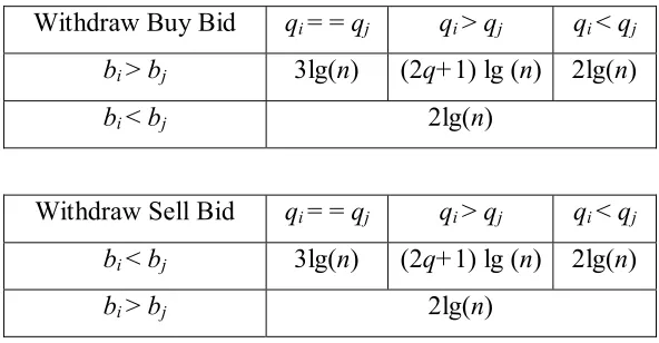
3.6. The 4-Heap Withdraw Action
Withdrawing an active bid is the opposite of inserting a new bid. The logic behind these operations is similar to the bid insert action. The only difference is the direction of bid movements, which is opposite to inserting a new bid. In the worst case, (2q+1) lg (n) operations take place when withdrawing an active bid as in Table 3.2.
Withdraw Buy Bid qi = = qj qi > qj qi < qj
bi > bj 3lg(n) (2q+1) lg (n) 2lg(n)
bi < bj 2lg(n)
Withdraw Sell Bid qi = = qj qi > qj qi < qj
bi < bj 3lg(n) (2q+1) lg (n) 2lg(n)
bi > bj 2lg(n)
Table 3.2. The worst case complexity analysis of the 4-Heap withdraw action.
3.7. The 4-Heap Clear Action
A clear action happens when emptying the transaction set Bin and Sin according to one
clearing price. Our implementation of the clear action is to set aside the bids in Bin and
Sin. This action takes constant time O (1). The clearing price can be set as the Mth price,
(M+1) st price, or by the kth double auction price [5].
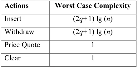
3.8. The Worst Case Complexity Analysis of the Four Auction Actions
Actions Worst Case Complexity
Insert (2q+1) lg (n)
Withdraw (2q+1) lg (n)
Price Quote 1
Clear 1
Table 3.3. The worst case complexity analysis of the four auctions actions in the 4-Heap algorithm.
Table 3.3 presents the worst case complexity for the four auction actions when applying the 4-Heap algorithm to manipulate bids. The insert and withdraw actions have the same worst case complexity (2q+1) lg (n), where q is quantity of the inserted or withdrawn bid. The price quote and clear actions take constant time O (1).
4. The Multi-unit Bid IPR Tree Algorithm
For the 4-Heap algorithm, when inserting a new buy bid into or withdrawing an active buy bid from Bin, or inserting a new sell bid into or withdrawing an active sell bid from
Sin, (2q+1) lg(n) operations occur in the worst case for the insert and withdraw actions.
Since the complexity of the 4-Heap algorithm price quote and clear actions are both constant time, if we reduce the number of qlg(n) operations in the insert and withdraw actions, the algorithm performance will be improved subject to the effects of constant factors in the implementation. Thus, we introduce a bid management algorithm based on the IPR tree structure.
4.1. The IPR Tree
The Internal Path Reduction tree is a height-balanced binary search tree. The internal path length is defined to be the sum of the depth of all the nodes in the tree. This parameter determines the tree balance and thus the tree height. By reducing the internal path length of a tree, the number of retrieval probes and the time to retrieve a node is reduced.
The IPR tree is rebalanced when the difference between the numbers of children down two branches exceeds some threshold k. There are four balance rotations to reduce the internal path length [Figure 4.1].
In the two single rotations, Nc refers to the number of children of the subtree C. Narefers
to the number of children of the subtree A. k is the balance parameter and represented by an integer. Single rotations occur when the number of children of the subtree C is greater than the number of children of the subtree A by k.
Figure 4.1. The four balance rotations in the IPR tree.
In the two double rotations, Nb refers to the number of children of the node b. It includes
the number of children of the subtree B1, the number of children of the subtree B2, and the node b. That is,
Nb = NB1 + NB2 + 1.
Na refers to the number of children of the subtree A. k is the balance parameter and
represented by an integer. Double rotations occur when the number of children of the node b is greater than the number of children of the subtree A by k.
4.2. Different Balanced Trees
Data Structure Average Case Worst Case
Binary Search Tree lg(n) n
AVL Tree lg(n) lg(n)
IPR Tree lg(n) lg(n)
Table 4.1. The complexity analysis for different tree structures in insert, look-up and withdraw operations.
Worst Case Complexity AVL Tree IPR Tree
Height ≤ 1.4402 lg(n) ≤1.4402 lg(n)
Internal path length ≥1.2793 n lg(n) ≥1.0515 n lg(n)
Table 4.2. The worst case complexity analysis for an AVL and an IPR tree [3].
We selected an IPR tree to represent our bid data structure because of its better performance in insert, look-up and withdraw operations when compared with other candidate binary search trees.
In Table 4.1, an AVL tree and an IPR tree are more efficient than a Binary Search Tree in the worst case. A Binary Search Tree is not a height-balanced tree. If the nodes are inserted in decreasing or increasing order, the insert, look-up and withdraw actions will traverse all the nodes in the tree. Thus, in the worst case, the complexity of these actions becomes linear O (n).
The height of an IPR tree is never worse than an AVL tree with the same number of nodes. The worst case performance for an IPR tree and an AVL tree is the same. From Table 4.2, the Internal Path Length of an IPR tree is about 10% better [3]. It means we need 10 percent fewer probes on the average to retrieve each node once with an IPR tree. This table shows an IPR tree is more efficient than an AVL tree.
An IPR tree also provides some flexibilities in that the degree of the tree imbalance can be varied by the parameter k. (Nc-Na > k and Nb-Na> k). The greater the value of k, the
greater will be the allowed imbalance. This in turn will reduce an IPR tree insertion effort though allowing longer insertion paths.
4.3. The IPR Tree Insert Action
When inserting a new bid, this new bid is wrapped up as a new node and placed into the bottom of an IPR tree branch. Insert actions assure the lower priority nodes are always in the left branches of an IPR tree; and the higher priority nodes are always in the right branches of an IPR tree.
Two pointers are introduced to keep track of the Mth and the (M+1) st prices. Similar to the Multi-unit Bid 4-Heap Algorithm, bid type, price and quantity are the main factors to determine the Mth and (M+1) st prices in an IPR tree. The challenge is to track how the Mth and (M+1) st price pointers move when inserting a new bid into or withdrawing an active bid from an IPR tree.
Two operations are applied in our IPR tree algorithm to keep track of the Mth and (M+1)st prices. One operation is move-up-q-units. This operation performs the same function as moving the Mth and (M+1) st price pointers upward by q units according to the nodes’ priority order. The other operation is move-down-q-units. This operation performs the same function as moving the Mth and (M+1) st price pointers downward by q units according to the nodes’ priority order. These two operations keep track of the Mth and (M+1) st price pointers’ movements as bids are inserted into or withdrawn from an IPR tree.
4.3.1. The Next Higher Priority Node of the Node T
For any node T, the next higher priority node refers to the lowest priority node among all the nodes that have higher priority than the node T in an IPR tree. How to find the next higher priority node plays an important role in the move-up-q-units operation. The move-up-q-units operation moves the Mth and (M+1) st price pointers upward by continuously finding the next higher priority node. Finding the next higher priority node is the key to move these two pointers correctly.
4.3.2. Examples for Finding the Next Higher Priority Node
Three examples are given to explain how to find the next higher priority node in an IPR tree. These examples also show the next higher priority node can reside in any place in an IPR tree.
Figure 4.2. The next higher priority node ---example 1.
$45
2
$50 3
Old Mth Price
$30 3
$43
2
$29
2
New Mth Price
$60
2
: :
$70 2
New Buy Bid
Example 1:
The next higher priority node of a node T is this node’s right child node. Figure 4.2 shows an example in which we have inserted a new buy bid with price at $70 for 2 units into an IPR tree. If we sort the entire bids in decreasing order according to the bid priority rules, to get the new Mth price we move the Mth price pointer up by 2 units. The new Mth price pointer will point at the bid with the price at $50. This bid resides in the old Mth price node’s right child node.
Figure 4.3. The next higher priority node ----example 2.
Example 2:
The next higher priority node of a node T is the leftmost child node of this node’s right branch. The right branch guarantees all the nodes in this branch has higher priority than the node T. The leftmost child assures this node has the lowest priority among this branch.
$45
2
$50 3
Old Mth Price
$30 3 $43 2 $29 2
New Mth Price $60 2 $49 3 $46 3 : : $70 2
New Buy Bid
In Figure 4.3, we have inserted a new buy bid with price at $70 for 2 units into an IPR tree. We move the old Mth price pointer up by 2 units in order to get the new Mth price. The new Mth price pointer will point at the bid with the price at $46. This bid resides in the leftmost child of the old Mth price node’s right branch.
Figure 4.4. The next higher priority node ----example 3.
Example 3:
The next higher priority node of a node T is this node’s parent node. For any node, if this node is in the right branches of an IPR tree, the child nodes in these branches always have higher priority than the parent nodes; if this node is in the left branches of an IPR tree, the parent nodes in these branches always have higher priority than the child nodes.
$45
2
$50 3
Old Mth Price
$30 3
$43
2
New Mth Price
$60
2
$49
3
$80
2
: :
$70 2
New Buy Bid
In Figure 4.4, we have inserted a new buy bid with price at $70 for 2 units into an IPR tree. Since the old Mth price node is in the left branch, the parent nodes in this branch always have higher priority than the child nodes. If we sort the entire bids in the decreasing order according to the bid priority rules, to get the new Mth price we move the Mth price pointer up by 2 units. The new Mth price pointer will point at the node with the price at $45, which is the first parent node that has higher priority than the old Mth price node. This node is old Mth price node’s next higher priority node.
4.3.3. The Algorithm for Finding the Next Higher Priority Node
The following algorithm generalizes how to find the node T’s next higher priority node in an IPR tree.
1. First check the node T’s right child node.
2. If the right child node exists, then check this right child node’s left child node. a. If the left child node does not exist, this right child node is the next higher
priority node.
b. If the left child node does exist, then traverse the left branch of this right child node to the leftmost child node. This leftmost child node is the next higher priority node.
3. If the right child node does not exist, then traverse the node T’s parents. The first parent that has higher priority than the node T is the next higher priority node.
4.3.4 The Previous Lower Priority Node of the Node T
For any node T, the previous lower priority node refers to the highest priority node among all the nodes that have lower priority than the node T in an IPR tree. How to find the previous lower priority node plays an important role in the move-down-q-units operation. The move-down-q-units operation moves the Mth and (M+1) st price pointers downward by continuously finding the previous lower priority node. To find the previous lower priority node is the key to move these two pointers correctly.
The following algorithm generalizes how to find the node T’s previous lower priority node.
1. Check the left child of the node T.
2. If the left child node does exist, check this left child node’s right child node. a. If the right child node does not exist, this left child node is the previous
lower priority node.
b. If the right child node does exist, traverse the right branch of this left child node to the rightmost child node. This rightmost child node is the previous lower priority node.
3. If the left child node does not exist, then traverse the node T’s parent nodes. The first parent node that has lower priority than the node T is the previous lower priority node.
4.3.5 Move-up-q-units Operation
Sometimes finding the next higher priority node or the previous lower priority node is not enough to generate the correct Mth and (M+1) st prices. The complexity is due to the new bid quantity.
Figure 4.5. Move-up-q-units example.
Figure 4.5 shows an example in which we have inserted a new buy bid at $70 for 10 units into an IPR Tree. To get the new Mth price we move the Mth price pointer up by 10 units according to the Mth price rule. The new Mth price pointer will point at the bid with the price at $60. This node does not reside in any of the positions we mentioned in section 4.3.2—Examples for Finding the Next Higher Priority Node. The explanation is there are many nodes that have higher priority than the old Mth price node and lower priority than the new buy node. The new buy bid quantity is much bigger than the quantities of those bids. Thus, the Mth price pointer must traverse several other bids before reaching the bid with the price at $60. In this Figure, we actually apply four times of finding the next higher priority node algorithm. The new buy bid quantity determines how many times to apply this algorithm.
$45
2
$50
3
Old Mth Price
$30 3
$43
2 New Mth Price
$60
2
$49
3
$80
2
: :
$70 10
New Buy Bid
4.3.6. Unit Counter
For each node, we keep a counter about the number of units in this node’s left and right subtrees. This counter helps us determine directly whether the new Mth and (M+1) st prices will reside in this node’s subtrees or this node’s parents. We can avoid traversing this node’s subtrees if this counter determines that the Mth or (M+1) st prices are in the parent nodes. This improvement avoids unnecessary computation.
Figure 4.6 shows each node’s internal structure. The unit counter parameter is used to record the number of units for this node’s left and right subtrees.
Figure 4.6. The unit counters in an IPR tree. Parent Bid ID Bid Type Bid Price Bid Quantity Unit Counter
Left Right Child Child
Parent Bid ID Bid Type Bid Price Bid Quantity Unit Counter
Left Right Child Child
Parent Bid ID Bid Type Bid Price Bid Quantity Unit Counter
Left Right Child Child Parent Bid ID Bid Type Bid Price Bid Quantity Unit Counter
Left Right Child Child
4.3.7. Move-up-q-units
After introducing the concepts of the next higher priority node and the unit counter, we present the move-up-q-units algorithm.
1. Set an integer counter n that is equal to the new buy bid quantity. And get the current Mth price node’s right branch unit counter.
2. While n is greater than zero.
a. If n is smaller than or equal to the right branch unit counter, continue finding the next higher priority node and subtract its quantity from n. If n is not greater than zero, this next higher priority node is the new Mth price node and the while loop stops.
b. If n is greater than the right branch unit counter, subtract the right branch unit counter from n. Find the first parent node that has higher priority than the current Mth price node.
i. If n is smaller than or equal to this parent node’s quantity, this parent node is the new Mth price node and the while loop stops. ii. If n is bigger than this parent node’s quantity, get this parent
node’s right branch unit counter, and continue the loops.
4.3.8. Move-down-q-units
Move-down-q-units operation has the similar logic as move-up-q-units operation. The only difference is we need to find the previous lower priority nodes instead of finding the next higher priority nodes.
4.3.9. The IPR Tree Insert Action Algorithm
For an IPR Tree insert action, we wrap the new bid into a new node, traverse one branch of the IPR tree and insert this new node at the bottom of this branch. Since adding the new node may change this IPR tree height, sometimes we have to rebalance the IPR tree according to the four balance rotation methods. If the new bid is a buy bid and this bid has higher priority than the current Mth price bid, or the new bid is a sell bid and this bid has lower priority than the current (M+1) st price bid, we have to update the Mth and (M+1) st price pointers by following the move-up-q-units or move-down-q-units operation.
In general, inserting a new node takes lg (n) time, balancing the IPR tree takes lg (n) time, and updating the Mth and (M+1) st price pointers in the worst case takes 2lg (n) time. So the worst case for the IPR tree insert action takes 4lg (n) time. Below is the IPR tree insert action algorithm:
1. Set a tree traversal pointer p point to the root node of the IPR tree. 2. While p is not null, compare this new node with the node pointed to by p.
a. If the new node has lower priority, reset p to point to the left child of this node pointed to by p. If p is null, insert this new node as the node’s left child and the while loop stops.
b. If the new node has higher priority, reset p to point to the right child of this node pointed to by p. If p is null, insert this new node as the node’s right child and the while loop stops.
3. For each node on the path from the parent of the newly inserted node to the root of the tree.
a. Determine if the associated subtree has more nodes to the right or left or neither to know whether to perform a left or right rotation.
b. If Nc-Na> k, then
i. Perform a single rotation in the proper direction.
ii. After a left or right rotation, check the subtree of the immediate left (right) descendant of the root of the rotated subtree for balance. If unbalanced, rotate and recursively test for and perform any additional rotations.
c. Else if Nb-Na> k, then
i. Perform a double rotation in the proper direction.
ii. Check both immediate descendants for an imbalance and recursively perform any needed rotations.
4. Check the data type of this new node,
a. If the new node is a buy node, compare this new node with the node pointed by the Mth price pointer,
i. If the new node has higher priority, apply the move-up-q-units operation in section 4.3.7.
ii. If the new node has lower priority, keep the current Mth price pointer. If this new buy node has higher priority than the node pointed by the (M+1) st pointer, update the (M+1) st price pointer to point to this new node.
b. If the new node is a sell node, compare this new node with the node pointed by the (M+1) st price pointer,
i. If the new node has lower priority, apply the move-down-q-units operation in section 4.3.8.
ii. If the new node has higher priority, keep the current (M+1) st price pointer. If this new node has lower priority than the node pointed by the Mth price pointer, update the Mth price pointer to point to this new node.
4.4. The IPR Tree Price Quote Action
Generating a price quote with the IPR tree algorithm is as straightforward as with the 4-Heap algorithm. Since the IPR Tree maintains two pointers to keep track of the Mth and (M+1) st prices, to get the price quote we just follow the two pointers and return the nodes’ prices. The complexity of the IPR tree price quote action is constant time O (1).
4.5. The IPR Tree Withdraw Action
The IPR tree withdraw action is opposite to its insert action. It traverses the tree to find the node, which takes lg (n) time. After finding the node, removing this node has to consider its left and right children. If the left and right children are not empty, a replacement node is needed to replace the withdrawn node in order to maintain the IPR tree parent and children relations.
Figure 4.7. Withdrawing a node from an IPR tree.
$45 2 $30 3 $43 2 $60 2 $49 3 $80 2 : : $50 3 $30 3 $43 2 $60 2 $49 3 $80 2 : :
(1) (2)
$50 3
In Figure 4.7(1), we want to withdraw the node at price $45 from an IPR tree. In order to maintain the valid parent and children relations, we move the node at price $43 to the empty slot. The IPR tree after the withdrawal is shown in Figure 4.7(2)
Not any node can replace the withdrawn node. The replacement node must be either the next higher priority node or the previous lower priority node. Finding such a replacement node takes lg (n) time.
If withdrawing a buy node that has higher priority than the node pointed by the Mth price pointer, or withdrawing a sell node that has lower priority than the node pointed by the (M+1) st price pointer, the Mth and (M+1) st price pointers have to be updated after withdrawing this node. This update at worst takes 2lg (n) time. In general, the complexity of the IPR tree withdraw action is 4lg (n).
4.6. The IPR Tree Clear Action
The IPR tree clear action traverses the tree and, according to each bid price and type, either keeps the bid in the tree or removes the bid from the tree. The action is comprised of a series of withdraw actions. Each withdraw action removes one bid in the transaction set from the tree. The clear action is based on the in-order traversal. In-order traversal traverses the tree from left to right and from bottom to top. It guarantees the nodes are traversed in ascending order.
When clearing the auction, 2nlg (n) time operations take place. Traversing the tree and removing the nodes from the tree takes n lg (n) time. After each bid removal, the tree has to be rebalanced according to the IPR tree balance parameter. The rebalance process in total also takes nlg (n) time.
When removing a node from the tree, sometimes we need to find a replacement node to keep the parent and children relations. In our implementation, we prefer the previous lower priority nodes compared with the next higher priority nodes to replace the removed nodes. The reason is lower priority nodes are visited first. For any removed node, its previous lower priority node has already been visited and kept in the tree. If we choose the next higher priority node to replace a removed node, this replacement node may be removed later from the tree. Thus increases the computation cost.
Below is the clear action algorithm:
1. Traverse the tree. Check to see whether the nodes belong to the transaction set according to the Mth and (M+1) st prices.
a. If a node belongs to the transaction set,
i. Find a replacement node by choosing the previous lower priority node. Swap the bid part between this node and the replacement node, and maintain the node’s parent and children relations.
ii. If the previous lower priority node is not found, find a replacement node by choosing the next higher priority node. Swap the bid part between this node and the replacement node, and maintain the node’s parent and children relations.
iii. Delete the replacement node from the tree by applying the same process as above.
b. If a node does not belong to the transaction set, keep the node in the tree.
c. If the child subtrees become unbalance according to the balance parameter, first balance the subtrees by applying the IPR tree balance rotations. Then traverse the tree from the parent of this node to the root node and continue balancing the tree according to the balance parameter.
4.7. The Worst Case Complexity Analysis of the Four Auction Actions
Actions Worst Case Complexity
Insert 4lg(n)
Withdraw 4lg(n)
Price Quote 1
Clear 2nlg(n)
Table 4.3. The worst case complexity analysis of the four auction actions in the IPR tree algorithm.
Table 4.3 lists the worst case complexity for the four auction actions when applying the IPR tree algorithm to manipulate bids. The insert and withdraw actions have the same worst case complexity 4lg (n). The price quote action is constant time O (1). The clear action takes 2nlg(n) time and is the worst among the four auction actions.
5. Experimental Evaluation of the Two Algorithms
These two algorithms are written in C++. We test these two algorithms on UNIX machines with the size of bids ranging from 10,000 to 90,000. We perform four experiments to evaluate the complexity of the auction actions and study the impact of number of bids, bid quantity, clear interval and bid distribution on algorithm performance. These comparisons use CPU time as a performance measurement, and the CPU time is measured in seconds.
5.1. The Impact of the Number of Bids on Algorithm Performance 0.23 0.51 0.81 1.09 1.41 1.71 2.11 2.43 2.77 0.10 0.19
0.31 0.42 0.54
0.69 0.82 0.93 1.05 0.00 0.50 1.00 1.50 2.00 2.50 3.00
1 2 3 4 5 6 7 8 9
Number of Bids (10,000)
CP U Ti me (s ec onds ) 4-Heap IPR Tree
Figure 5.1. The impact of number of bids on algorithm performance.
Number of Bids The 4 Heap(seconds) The IPR Tree(seconds) (4 Heap / IPR Tree) Times
10000 0.23 0.10 2.438
20000 0.51 0.19 2.705
30000 0.81 0.31 2.570
40000 1.09 0.42 2.587
50000 1.41 0.54 2.609
60000 1.71 0.69 2.481
70000 2.11 0.82 2.565
80000 2.43 0.93 2.609
90000 2.77 1.05 2.627
Table 5.1. The actual CPU time with different number of bids.
This experiment uses randomly generated multi-unit bids. High price bids and low price bids are mixed. Each bid quantity is also randomly generated between 1 and 10. 9 tests are performed with the number of bids ranging from 10,000 to 90,000.
Table 5.1 shows as the number of bids increases, the CPU time for both algorithms’ insert action also increases. The IPR tree algorithm is about three times faster than the 4-Heap algorithm. This result is due to their insert action complexity. For the 4-4-Heap algorithm, when a new bid arrives, in the worst case (2q+1) lg (n) operations take place. For the IPR tree algorithm, the worst case for inserting a new bid is 4lg (n).
For example, if we insert a new buy bid with quantity 6 into Bin. If we apply the 4-Heap
algorithm, in the worst case, 13 lg (n) operations take place. If we apply the IPR tree algorithm, in the worst case 4 lg (n) operations take place. The IPR tree algorithm is about 3 times faster than the 4-Heap algorithm, that is 13lg (n) ≈ 3 * 4lg (n). This explains why the IPR tree algorithm is more efficient than the 4-Heap algorithm for the insert action.
5.2. The Impact of Bid Quantity on Algorithm Performance
Set Bid Quantity
The 4-Heap (seconds)
The IPR Tree (seconds)
1 1 0.229 0.085
2 1-100 0.233 0.101
3 1-500 0.246 0.177
4 1-1000 0.253 0.205
5 Exponential
Distribution 0.227 0.125
Table 5.2. The actual CPU time with different bid quantity.
Table 5.2 shows results for testing five sets of 10,000 bids with different bid quantity. The first set includes 10,000 single unit bids. The quantity of the bids in the second set is a randomly generated number between 1 and 100. For the third set, the quantity is a randomly generated number between 1 and 500. The quantity of the bids for the fourth set is between 1 and 1000. The fifth set is exponential distribution.
As the variations in bid quantity increases, the CPU time increases for both the 4-Heap algorithm and the IPR tree algorithm. Larger bid quantity variations have negative impact on the two algorithms’ performance.
For example, suppose there is one auction with 100 bids. Each bid quantity is one. We insert a new buy bid into Bin using 4-Heap algorithm. If this new buy bid quantity is one,
in worst case 3lg (n) operations take place. If this new bid quantity is 10, in worst case 21 lg (n) operations take place. The bigger variation in bid quantity incurs more bid movements, thus increases the computation cost.
The same logic applies to the IPR tree algorithm. For the IPR tree algorithm, the variation in bid quantity increases, the possibility to traverse more nodes becomes greater.
Exponential distribution of bid quantity refers to the situation as the bid quantity x increases, the possibility of such bids distributed in the auction P(x) decreases, and the cumulative distribution of such bids in the auction D(x) is close to 1.
Figure 5.2. The exponential distribution.
Given a rate of change , the formula are:
In our exponential distribution experiment, we generate the bid quantity according to the formulas q = ln (p)/ -λ where λ=0.001, and p is any random number between 0 and 1. The quantity generated is between 1 and 9,999. From Table 5.2, the CPU time of the exponential distribution is close to the CPU time of the random distribution of bid quantity between 1 and 100. The reason is small quantity bids generated by formulas q = ln (p)/ -λ occupy a much larger percentage than large quantity bids.
5.3. The Impact of the Clear Action on Algorithm Performance
Clear Interval
The 4-Heap (seconds)
The IPR Tree (seconds)
1000 0.235 0.082
5000 0.236 0.076
10000 0.225 0.071
Table 5.3. The actual CPU time for different clear intervals.
Bid Size
The 4-Heap (seconds)
The IPR Tree (seconds)
Insert & Clear (seconds) 90000 2.690 0.975
Clear (seconds) 90000 0.004 0.144
Clear / Insert & Clear
(percentage) 90000 0.159% 14.769%
Table 5.4. The percentage of clear action CPU time.
Table 5.3 shows the clear action slows the performance for both the 4-Heap algorithm and the IPR tree algorithm. For the IPR tree algorithm, the worst case complexity of the clear action is 2nlg (n). The clear action for the 4-Heap algorithm in the worst case takes constant time O (1).
From Table 5.4, the clear action occupies 14.8 % of the total CPU time for the insert and clear action combined in the IPR tree algorithm. In the 4-Heap algorithm, the clear action occupies 0.2% of the total CPU time for the insert and clear actions combined.
However when considering the actual CPU time for the two algorithms in Table 5.3, the IPR tree algorithm takes only 0.975 seconds to insert 90,000 bids and clear its transaction set. The 4-Heap algorithm takes 2.69 seconds to insert 90,000 bids and clear its transaction set. Even though the actual clear action takes the IPR tree algorithm 0.144 seconds and takes the 4-Heap algorithm 0.004 seconds, the IPR tree algorithm is still more efficient than the 4-Heap algorithm in total CPU time spent when the insert and clear actions are combined.
5.4. The Impact of Bid Ordering on Algorithm Performance
Figure 5.3. The diverge and converge of bid distributions.
In real market, bids do not always occur randomly. We don’t know what real buyers do, so we simulate two scenarios. A price converge happens when buyers and sellers try to win the auction by biding their prices that are very close to the auction clearing price. A price diverge occurs when buyers and sellers’ bid prices are away from the auction clearing price.
We test 5 scenarios to compare the two algorithms’ performance. In these five scenarios, the number of bids is 10,000. The quantity of each bid is randomly generated between 1 and 10.
Scenario
Bid Distributions The 4-Heap
(seconds)
The IPR Tree (seconds)
Scenario 1 Diverge 0.131 9.808
Scenario 2 Diverge 0.122 4.911
Scenario 3 Converge 0.121 4.831
Scenario 4 Converge 0.507 4.865
Scenario 5 Random 0.492 0.089
Table 5.5. The actual CPU time for different bid distributions.
Figure 5.4. The different bid converge and diverge distributions.
The horizontal axis in Figure 5.4 is bid order, and the vertical axis is bid price. The shaded area identifies bids that transact. For scenario 1, 2, 3, and 4, the bid price is increased or decreased by 1 for each new bid.
The size of the transaction set has big impact on the IPR tree algorithm performance. The CPU time doubles when the size of the transaction set doubles. For scenario 1, all 10,000 bids are in the transaction set, while for scenarios 2 and 4, the transaction set has 5,000 bids. The increased CUP time is necessary because bids added to the transaction set are the ones that require Mth and (M+1) st prices to move.
The random bid distribution means high price bids and low price bids are mixed. From Table 5.5, the IPR tree algorithm is more efficient than the 4-Heap algorithm if the bids are randomly distributed.
For the IPR tree algorithm, the increasing or decreasing arrival order of bids has a big negative impact on performance. When the bids are arrived in either of these two orders, the tree becomes a linear chain of nodes, and the same operations take linear worst case time. The performance suffers due to more CPU time spent on traversal, insertion and balance. The CPU time for these scenarios is much greater than the random bid distribution scenario.
For the 4-Heap algorithm, the increasing or decreasing arrival order of bids has a big positive impact on CPU time in various scenarios except scenario 4. Below we explain the differences among these scenarios.
In scenario 3, buy and sell bids are not in the transaction set, thus there is no involvement with Sin and Bin heaps. All the sell bids are in Sout and Sout is a min-heap structure. All the
buy bids are in Bout and Bout is a max-heap structure. The sell bids are arrived in
decreasing order and have already maintained the min-heap structure. The buy bids are arrived in increasing order and have already maintained the max-heap structure. Since no further operations are needed to manipulate the heap property for Sout and Bout, the CPU
time is smallest among the five scenarios. Similar logic explains why scenarios 2 and 3 both have better performance than the random bid distribution.
In scenario 4, the first 5,000 bids are not in the transaction set. The sell bids are in Sout
and the buy bids are in Bout. The later 5,000 bids are in the transact set. Repetitious bid
insert and withdraw actions take place among the four heaps for the later 5,000 bids. For example, if the 5001st bid is a buy bid, the 4-Heap algorithm pops one sell bid from Sout
and pushes this bid into Sin. If the 5002nd bid is a sell bid, the 5002nd bid is inserted into
Sin, and the original bid in Sin has to be removed and reinserted into Sout. This repetition
explains the biggest CPU time spent compared with other scenarios.
6. Conclusions
Compared with the 4-Heap algorithm, the IPR tree algorithm has some advantages. In the IPR tree algorithm, the bids can be inserted and cleared much faster than in the 4-Heap algorithm if the bids are randomly distributed. In addition, the IPR tree algorithm has storage advantages. The IPR tree algorithm requires much less memory to process the bids. In our implementation, we use arrays to represent the four heaps. The 4-Heap algorithm memory allocation is about 4 times as big as the IPR tree algorithm memory allocation.
The IPR tree allows stored data to be processed in many different ways relatively efficiently, such as in-order traversal, pre-order traversal, and post-order traversal. The heap structure does not provide this benefit.
However, the IPR tree algorithm has some constraints. If the bids arrive in increasing or decreasing order, the algorithm’s performance deteriorates quickly.
Thus, there is no definite answer as to which algorithm is better. Whenever we apply auction algorithms in real world applications, we need to study the environment characteristics, including the expected bid distributions and the auction’s clear policies. According to these studies, we can choose the proper algorithm to achieve our goal – providing a fast and efficient online service to customers.
7. References
[1] Peter R.Wurman, William E.Walsh and Michael P. Wellman. Flexible Double Auctions for Electronic Commerce: Theory and Implementation Decision Support Systems, 24:1 pages 17-27,1998.
[2] Alan L.Tharp. File Organization and Processing, John Wiley & Sons, 1988.
[3] Thomas H. Cormen, Charles E.Leiserson, Ronoal L. Rivest and Clifford Stein Introduction to Algorithms, MIT press, 1990.
[4] Daniel Friedman and John Rust, editors. The Double Auction Market: Institutions, Theories, and Evidence. Addison Wesley, 1993.
[5] Kevin A. McCabe, Stephen J. Rassenti, and Vernon L. Smith. Auction institutional design: Theory and behavior of simultaneous multiple-unit
generalizations of the Dutch and English auctions. American Economic Review, 80(5):1276-1283, 1990