Advanced Statistical Methods for Complex Longitudinal Data.

(1)

ABSTRACT

VOCK, DAVID MICHAEL. Advanced Statistical Methods for Complex Longitudinal Data. (Under the direction of Marie Davidian and Anastasios A. Tsiatis.)

Longitudinally collected data play an important role in many biomedical applications. As researchers have greater capacity to collect and store large amounts of data over time, biomedical research has shifted from trying to understand the effects of therapy at a single time point, to a more nuanced understanding of how therapy, which could change over time, longitudinally affects a patient. However, many standard methods of analyzing longitudinal data are not adequate to address questions of interest.

The first half of the thesis addresses methodological challenges when the longitudinally collected response may be censored. Mixed models are commonly used to represent longitudinal or repeated measures data. An additional complication arises when the response is censored, for example, due to limits of quantification of the assay used. While Gaussian random effects are routinely assumed, little work has characterized the consequences of misspecifying the random effects distribution nor has a more flexible distribution been studied for censored longitudinal data. We show that, in general, maximum likelihood estimators will not be consistent when the random effects density is misspecified, and the effect of misspecification is likely to be greatest when the true random effects density deviates substantially from normality and the number of non-censored observations on each subject is small. We develop a mixed model framework for censored longitudinal data in which the random effects are represented by the flexible seminonparametric (SNP) density and show how to obtain estimates in SAS procedure NLMIXED. Simulations show that this approach can lead to reduction in bias and increase in efficiency relative to assuming Gaussian random effects. The methods are demonstrated on data from a study of hepatitis C virus.

(2)

(3)

(4)

Advanced Statistical Methods for Complex Longitudinal Data

by

David Michael Vock

A dissertation submitted to the Graduate Faculty of North Carolina State University

in partial fulfillment of the requirements for the Degree of

Doctor of Philosophy

Statistics

Raleigh, North Carolina 2012

APPROVED BY:

Dennis D. Boos Daowen Zhang

Marie Davidian

Co-chair of Advisory Committee

(5)

DEDICATION

(6)

BIOGRAPHY

Originally from Wheaton, Illinois, David M. Vock is the son of David J. and Janice Vock. David graduated from Wheaton North High School in 2003 and was captain of the two-time Illinois state champion scholastic bowl team for Wheaton North. After high school, David attended St. Olaf College in Northfield, Minnesota where he majored in mathematics and chemistry with a concentration in statistics. While at St. Olaf College, he had the opportunity to study biostatistics and collaborate with World Health Organization researchers in Geneva, Switzerland. David was elected to Phi Beta Kappa and graduated summa cum laude with a Bachelor of Arts degree and distinction in statistics from St. Olaf in 2007.

Interested in many different academic disciplines, David decided to pursue graduate studies in statistics because, in the words of John Tukey, he could “play in everyone’s backyard.” He began his graduate studies in 2007 at North Carolina State University in Raleigh, North Carolina. David received a Master of Statistics degree from Noth Carolina State University in 2009. He actively collaborates with medical researchers at Duke Clinical Research Institute. David’s collaborative work has largely focused on hepatitis C and lung transplantation research and has motivated much of his methodological research in longitudinal data analysis, causal inference, and dynamic treatment regimes. He intends to complete his Ph.D. under the direction of Drs. Marie Davidian and Anastasios A. Tsiatis.

(7)

ACKNOWLEDGEMENTS

Many people have helped and guided me through my graduate studies and dissertation research. I would like to express my gratitude to a few people below while acknowledging that many more people deserve praise.

I would like especially to thank my advisors, Drs. Marie Davidian and Butch Tsiatis. They have showed incredible patience in allowing me to explore various research lines and I am very thankful for their latitude. Their expertise and gentle guidance have been immensely helpful in completing this work. I also would like to thank them for offering me a research assistantship to support me during most of my time at North Carolina State. Mostly, I would like to express my gratitude to them for being great faculty role models and mentors. They have guided me through the peer-review process, made sure that I would gain teaching experience, and given me valuable advice on searching for academic jobs. Butch and Marie have shown me how to contribute to interdisciplinary research and how to use collaborative research to motivate methodological work.

I wish to thank all the faculty and staff at North Carolina State that have helped me along the way. I want to thank especially the Directors of the Statistics Graduate Program during my first years at North Carolina State, Drs. Pam Arroway and Jacqueline Hughes-Oliver, for being patient in answering all my questions and taking the time to help me find interesting funding opportunities. I am also appreciative of all the advice Dr. Eric Laber has given me about how to interview for faculty jobs and how to be a successful junior faculty member. Finally, I would like to thank Drs. Dennis Boos and Daowen Zhang for serving on my committee, writing letters of recommendation, and being wonderful teachers of some of the most interesting and useful courses I have taken in graduate school, especially Advanced Inference and Mixed Models and Variance Components.

I am also thankful for the opportunity to work with Karen Pieper at Duke Clinical Research Institute. She has been an invaluable resource on how to work with clinical investigators and artfully explain advanced methodology to a broad audience. I have learned a lot from her ability to prioritize the most urgent needs of a statistical analysis and to cajole subject area experts to “buy-in” to rigorous statistical analysis. In addition, I would like to thank all the clinical investigators that I have worked with at Duke. Besides teaching me a lot about their own area of research, they have been patient and nurturing.

(8)

(9)

LIST OF TABLES

Table 1.1 Proportion of subjects by number of non-censored observation for the four random effects densities considered in the simulations withq = 2 described in Section 1.5. . . 12 Table 1.2 Simulation results when Gaussian random effects were assumed for all

models regardless of the true distribution of the random effects. The sim-ulation included 500 data sets with 500 subjects each. MC Avg: Monte Carlo average of the parameter estimates; MC SD: Monte Carlo standard deviation of the parameter estimates; Avg SE: Average of the standard error estimates; CP: Monte Carlo coverage probability of the 95 percent Wald-type confidence intervals. . . 13 Table 1.3 Proportion of subjects by number of non-censored observation when the

true random effects density was bimodal and the time points where data were collected was varied. tA= (0,1,2,3,4)T;tB = (0,1,2,3,3.5,4,4.5)T;

tC = (−2,−1,0,1,2,3,4)T. . . 14

Table 1.4 Simulation results when Gaussian random effects were assumed for the bimodal random effects but ti in (1.2) was varied. The simulation

in-cluded 500 data sets with 500 subjects each. tA = (0,1,2,3,4)T; tB =

(0,1,2,3,3.5,4,4.5)T; tC = (−2,−1,0,1,2,3,4)T; MC Avg: Monte Carlo

average of the parameter estimates; MC SD: Monte Carlo standard devi-ation of the parameter estimates; Avg SE: Average of the standard error estimates; CP: Monte Carlo coverage probability of the 95 percent Wald-type confidence intervals. . . 15 Table 1.5 Proportion of time K was selected using AIC, HQIC, and BIC when the

SNP density was used to model the random effects density. The simulation included 500 data sets with 500 subjects each. . . 16 Table 1.6 Simulation results when the SNP density was used to model the random

effects density. Models with K = 0, K = 1, and K = 2 were fit and K was selected using HQIC. The simulation included 500 data sets with 500 subjects each. MC Avg: Monte Carlo average of the parameter estimates; MC SD: Monte Carlo standard deviation of the parameter estimates; Avg SE: Average of the standard error estimates; Ratio MSE: Ratio of the Monte Carlo mean square error between K = 0 and K selected by the HQIC. . . 17 Table 1.7 Proportion of responses censored at each time point for the 811 patients

with CT genotype in the IDEAL trial. . . 18 Table 1.8 Proportion of subjects by number of uncensored viral load measurements

for the 811 patients with the CT genotype in the IDEAL trial. . . 18 Table 1.9 Information criteria and parameter estimates from fitting model (1.10)

concerning the IDEAL study with K= 0, K= 1, and K= 2 . . . 19 Table 1.10 Parameter estimates, standard errors, and a 95 percent Wald-type

(12)

Table 2.1 Summary of the parameter estimates forθ0 by estimator from 1,000 Mote Carlo simulations when the number of organs allocated was 1,250. Con-verge: Proportion of Monte Carlo datasets the estimator converged; MC mean: Monte Carlo average of the parameter estimates; MC SD: Monte Carlo standard deviation of the parameter estimates; Avg SE: Average of the standard error estimates; Ratio Avg SE:SD: Ratio of the average of the standard error estimates to the standard deviation of the param-eter estimates; Ratio MSE: Ratio of the average squared error of the fac estimates to the average squared error of the estimates of the given es-timator; CP: Monte Carlo coverage probability of 95 percent Wald-type confidence intervals. Approximate standard errors for the values in the col-umn MC Mean ranged from 0.0039 to 0.0086, the colcol-umn MC SD ranged from 0.0027 to 0.0061, the column Avg SE ranged from 0.0040 to 0.0092, the column Ratio Avg SE:SD ranged from 0.045 to 0.045, the column Ra-tio MSE ranged from 0.033 to 0.27, the column CP ranged from 0.0061 to 0.015. The true value ofθ0 is −0.10. . . 48 Table 2.2 Summary of the parameter estimates forθ1 by estimator from 1,000 Mote

(13)

Table 2.3 Summary of the parameter estimates forθ0 by estimator from 1,000 Mote Carlo simulations when the number of organs allocated was 2,500. Con-verge: Proportion of Monte Carlo datasets the estimator converged; MC mean: Monte Carlo average of the parameter estimates; MC SD: Monte Carlo standard deviation of the parameter estimates; Avg SE: Average of the standard error estimates; Ratio Avg SE:SD: Ratio of the average of the standard error estimates to the standard deviation of the param-eter estimates; Ratio MSE: Ratio of the average squared error of the fac estimates to the average squared error of the estimates of the given es-timator; CP: Monte Carlo coverage probability of 95 percent Wald-type confidence intervals. Approximate standard errors for the values in the col-umn MC Mean ranged from 0.0029 to 0.0061, the colcol-umn MC SD ranged from 0.0021 to 0.0043, the column Avg SE ranged from 0.0029 to 0.0067, the column Ratio Avg SE:SD ranged from 0.045 to 0.045, the column Ra-tio MSE ranged from 0.015 to 0.13, the column CP ranged from 0.0061 to 0.016. The true value ofθ0 is −0.10. . . 50 Table 2.4 Summary of the parameter estimates forθ1 by estimator from 1,000 Mote

Carlo simulations when the number of organs allocated was 2,500. Con-verge: Proportion of Monte Carlo datasets the estimator converged; MC mean: Monte Carlo average of the parameter estimates; MC SD: Monte Carlo standard deviation of the parameter estimates; Avg SE: Average of the standard error estimates; Ratio Avg SE:SD: Ratio of the average of the standard error estimates to the standard deviation of the parameter estimates; Ratio MSE: Ratio of the average squared error of the fac esti-mates to the average squared error of the estiesti-mates of the given estimator; CP: Monte Carlo coverage probability of 95 percent Wald-type confidence intervals. Approximate standard errors for the values in the column MC Mean ranged from 0.00019 to 0.00027, the column MC SD ranged from 0.00014 to 0.00019, the column Avg SE ranged from 0.00019 to 0.00035, the column Ratio Avg SE:SD ranged from 0.045 to 0.045, the column Ra-tio MSE ranged from 0.042 to 0.090, the column CP ranged from 0.0033 to 0.011. The true value ofθ1 is −0.05. . . 51 Table 2.5 Parameter estimates for the model of the propensity to receive an

(14)

Table 2.6 Parameter estimates of the scale accelerated failure time model for the ef-fect of lung transplantation. Group A: primarily COPD; Group B: primar-ily pulmonary hypertension; Group C: primarprimar-ily CF; Group D: primarprimar-ily IPF; Single LTx: single lung transplantation. The reference for Private In-surance and Medicare InIn-surance is Medicaid or other public funding for payment. LAS has been centered at 30, so the interpretation of the inter-cept term is the log acceleration factor at a LAS of 30. . . 60 Table B.1 Conversion between the notation used in Section 1 and the names used in

the example code. . . 77 Table C.1 Proportion of subjects by the number of non-censored observations for the

four random effect densities considered in the simulations with q= 1. . . . 82 Table C.2 Simulation results when Gaussian random effects were assumed for all

models regardless of the true distribution of the random effects. The sim-ulation included 500 data sets with 500 subjects each. MC Avg: Monte Carlo average of the parameter estimates; MC SD: Monte Carlo standard deviation of the parameter estimates; Avg SE: Average of the standard error estimates; CP: Monte Carlo coverage probability of the 95 percent Wald-type confidence intervals. . . 83 Table C.3 Proportion of time K was selected using AIC, HQIC, and BIC for q = 1

simulations when SNP was used to estimate the random effects. . . 84 Table C.4 Simulation results when SNP was used to estimate the random effects for

q= 1 simulations. Models with K= 0, K = 1, andK = 2 were fit andK was selected using HQIC. The simulation included 500 data sets with 500 subjects each. MC Avg: Monte Carlo average of the parameter estimates; MC SD: Monte Carlo standard deviation of the parameter estimates; Avg SE: Average of the standard error estimates; Ratio MSE: Ratio of the Monte Carlo mean square error between K = 0 and K selected by the HQIC. . . 85 Table I.1 Quantile (years) of the simulated residual life had the patient never been

(15)

LIST OF FIGURES

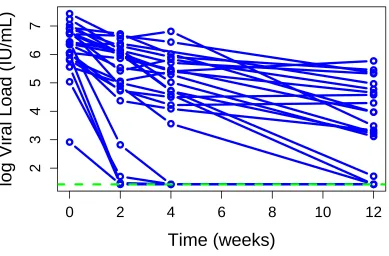
Figure 1.1 Trajectory of log₁₀viral load of 25 randomly selected subjects with geno-type CT from the IDEAL study. The lower limit of quantification, 1.431 log₁₀ IU/mL, is shown in the green dotted line. For graphical purposes, the lower limit of quantification was imputed for the censored responses. . 2 Figure 1.2 Contour plot of the true random effects densities from the “skewed” and

“bimodal” scenarios considered in the simulation described in Section 1.5. In each case, the densities were a 70-30 mixture of two normals. . . 21 Figure 1.3 Average estimated contour and marginal density plots from fitting 500

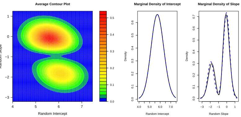
data sets with “skewed” random effects where the density was assumed to follow the SNP density with K selected by HQIC. The blue dotted lines on the marginal density plots are the true marginal density. The true bivariate random effects density is plotted in Figure 1.2 and described in Section 1.5. . . 21 Figure 1.4 Average estimated contour and marginal density plots from fitting 500

data sets with “bimodal” random effects where the density was assumed to follow the SNP density with K selected by HQIC. The blue dotted lines on the marginal density plots are the true marginal density. The true bivariate random effects density is plotted in Figure 1.2 and described in Section 1.5. . . 22 Figure 1.5 Contour plot of the bivariate density estimate and marginal density

es-timates for the subject-specific intercepts and slopes with K = 2 from model (1.10) concerning the IDEAL study. . . 23 Figure 2.1 Plot of ∆∗_ij(θ,F_j) and ˜V_ij∗(θ,F_j) as a function of ˜Rij where Cij∗(θ,Fj) =

500 and = 50. These are the “smooth” approximations to ∆ij(θ,Fj) =

I{R˜ij(θ) < Cij∗(θ,Fj)} and ˜Vij(θ,Fj) = min{R˜ij(θ), Cij∗(θ,Fj)},

respec-tively. . . 57 Figure 2.2 Histogram of all LAS scores each time an organ was offered (left) and

LAS scores at transplantation for those patients that were transplanted (right). . . 57 Figure 2.3 Kaplan-Meier residual survival curves for patients from the time of listing

(16)

Figure 2.4 Logarithm of the estimated scale acceleration factor in the transformation model for the causal effect of lung transplantation in Group A (primarily COPD, left) and Group D (primarily IPF, right) by LAS and transplan-tation type. The curves here are drawn for patients under 60 years of age, not in UNOS regions 6-8, and not paying for the transplant through pri-vate insurance or Medicare. We emphasize that negative (positive) values of the log scale factor suggest that transplantation increases (decreases) lifespan. The histogram in the background gives the number of patients transplanted for that range of LAS and native disease group. . . 61 Figure 2.5 Kaplan-Meier survival curves of the transformed residual lifetime for all

(i, j) pairs by LAS group and native disease. The rows correspond to native disease groups A, C, and D from top to bottom. The solid blue line corresponds to all (i, j) pairs wheredNij = 1 and the red dotted line

corresponds to all (i, j) pairs wheredNij = 0. If the transformation model

has been correctly specified then the two lines should be approximately the same. . . 62 Figure C.1 Estimated random effects density for each of the four random effect

den-sities considered (clockwise from upper left: normal, t5, bimodal, and skewed) when SNP was used to estimate the random effects and K was selected using HQIC. The estimated density is plotted for 100 randomly selected Monte Carlo data sets. The truth is superimposed in red, and the average of all 500 Monte Carlo data sets is superimposed in blue. . . . 86 Figure C.2 Histogram of the estimated variance of the random effect when SNP was

used to estimate the random effects density and the true random effect density was t5 (left). The estimated random effects densities for those data sets where the estimate of var(b0i) is greater than 4 are also plotted

(right). . . 87 Figure I.1 Logarithm of rate parameter from the exponential distribution used to

(17)

Chapter 1

Mixed Model Analysis of Censored

Longitudinal Data with Flexible

Random Effects Density

1.1

Introduction

Longitudinal or repeated measures data are commonly represented by mixed effects models. A complication occurs when the response is censored for some of the observations, which often arises when assay measures are collected over time and the assay procedure is subject to limits of quantification (Hughes, 1999; Jacqmin-Gadda et al., 2000; Wu, 2002; Gray et al., 2004; Wang and Fygenson, 2009, and references therein).

As an example, we consider data from the Individual Dosing Efficacy versus Flat Dosing to Assess Optimal Pegylated Interferon Therapy (IDEAL) study, which tracked the viral load progression of treatment-naive patients with hepatitis C (Thompson et al., 2010). One objective was to characterize the viral load decline in patients receiving standard treatment, pegylated interferon-alpha and ribavirin, over the first twelve weeks of treatment. Within-subjects, the trajectory of the log₁₀ viral load over the first 12 weeks is approximately linear, but responses were censored from below at 1.431 log₁₀ IU/mL, the lower limit of quantification of the assay used. Over the first 12 weeks, 10.5 percent of all observations were censored, and 35.2 percent were censored at week 12. The trajectories of 25 randomly selected subjects are shown in Figure 1.1.

(18)

0

2

4

6

8

10

12

2

3

4

5

6

7

Time (weeks)

log Vir

al Load (IU/mL)

● ● ● ● ● ● ● ● ● ● ● ● ● ● ● ● ● ● ● ● ● ● ● ● ● ● ● ● ● ● ● ● ● ● ● ● ● ● ● ● ● ● ● ● ● ● ● ● ● ● ● ● ● ● ● ● ● ● ● ● ● ● ● ● ● ● ● ● ● ● ● ● ● ● ● ● ● ● ● ● ● ● ● ● ● ● ● ● ● ● ● ● ● ● ● ● ● ●

(19)

accounts for the censoring and obtain the maximum likelihood estimates (MLE). Substantial research has gone into efficient methods to solve for the MLE. Hughes (1999) developed a Monte Carlo Expectation-Maximization (MCEM) estimation procedure to obtain the MLE for linear mixed effects models with censored responses. Wu (2002) extended the work of Hughes by devel-oping a EM algorithm for nonlinear mixed-effects models with censored responses that allowed for covariates to be measured with error. Wu (2004) further extended the EM algorithm to joint models of multiple longitudinal processes when the responses may be censored. Vaida and Liu (2009) derived a closed form expression for the expectation step rather than use Monte Carlo simulation, which greatly reduced the computational time. The estimation procedure developed by Vaida and Liu (2009) is available in the R package lmec.

Other computational approaches have been proposed besides the EM algorithm. Fitzger-ald et al. (2002) implemented a multiple imputation approach that avoids maximization of a censored likelihood. Jacqmin-Gadda et al. (2000) noted that the full likelihood is the product of the marginal density of the non-censored responses and the conditional distribution of the censored responses, evaluated at the limit of detection, given the non-censored responses. The authors used numerical integration to estimate the conditional distribution and then combined the Simplex algorithm and the Marquardt algorithm in the Fortran language to solve for the MLE. In contrast, both Thi´ebaut and Jacqmin-Gadda (2004) and Lyles et al. (2000) approxi-mate the full likelihood of mixed effect model by numerically integrating over the random effects densities and then using standard optimizers to obtain parameter estimates.

Previous methods cited above using this full-likelihood approach have all assumed Gaussian random effects and intra-subject error. While intra-subject error may be reasonably assumed to be normally distributed, the assumption of Gaussian random effects may be too restrictive in many applications. In the IDEAL study, some patients do not respond to treatment while others show marked declines in the viral load, so the distribution of subject-specific slopes is unlikely to be approximately Gaussian.

(20)

2001; Agresti et al., 2004; Liti`ere et al., 2008). The potential effect of misspecification of the random effects distribution when the response is censored has not been examined.

A variety of methods have been proposed to relax the Gaussian assumption for the random effects (Magder and Zeger, 1996; Verbeke and Lesaffre, 1997; Kleinman and Ibrahim, 1998; Aitkin, 1999; Zhang and Davidian, 2001; Chen et al., 2002; Lee and Thompson, 2008; Ho and Hu, 2008; Komarek and Lesaffre, 2008; Lin and Lee, 2008; Bandyopadhyay et al., 2010; Lachos et al., 2010); however, none of these methods has been implemented for censored longitudinal data. For linear mixed models, Zhang and Davidian (2001) assumed the random effects follow a “smooth” density that can be represented by the seminonparametric (SNP) formulation proposed by Gallant and Nychka (1987). They showed the log likelihood can be written in a closed form leading to straightforward estimation.

We show how the SNP representation can be implemented for the random effects density in linear mixed models when the response is potentially censored. In Section 1.2, we formulate the censored-response mixed model with Gaussian random effects and show that incorrectly assuming the random effects are Gaussian leads to inconsistent estimators of model parameters. In addition, we suggest general scenarios where estimation is likely to be particularly poor. In Section 1.3, we discuss the censored-response linear mixed model, where the random effects are assumed to follow a smooth, continuous density and introduce the SNP representation. Section 1.4 describes how to fit the SNP model using SAS procedure NLMIXED, how to select the degree of flexility in the model, and how to choose starting values. Section 1.5 presents the results of several simulations. In Section 1.6, we illustrate the method by application to data from the IDEAL study.

1.2

Gaussian Linear Mixed Model with Censored Response

For ease of presentation, we assume responses are potentially left-censored; developments are easily generalized to right- or interval-censored data. LetYij,i= 1, . . . , mand j= 1, . . . , ni be

thejth response for subjectithat would have been been observed had there been no censoring. Consider the usual linear mixed model for longitudinal data

Yij =vTijδ+sTijαi+ij =xTijβ+sTijbi+ij, (1.1)

where vij = (xTij, sTij)T; δ = (βT, γT); bi = γ+αi; β and γ are the p- and q-dimensional fixed

effects parameters associated with covariatesxij andsij, respectively;αiare theq-dimensional,

mean zero subject-specific random effect vectors associated with covariates sij, independent

acrossi; andij iid

∼ N(0, σ2) are the intra-subject error, which are independent ofαi. We adopt

(21)

asbi =µ+RZi, whereµis a (q×1) vector,R is a (q×q) lower triangular matrix, and Zi is a

(q×1) vector of random effects. Typically, Zi are assumed to follow a standard q-dimensional

normal distribution, which impliesbi are normally distributed with meanµ=γ and covariance

matrix var(αi) =RRT.

As an example, a special case of (1.1) is the linear random coefficient model with baseline covariatexi given by

Yij =xiβ+b0i+b1itij+ij, (1.2)

wherebi = (b0i, b1i)T and sij = (1, tij)T.

Due to left-censoring, we observe Qij which takes the value Yij for Yij > lij and takes

the value lij, the known lower limit of quantification for the jth response on subject i,

oth-erwise. Letting r = vech(R) be the non-zero elements of R, the parameters of interest are θ= (βT, µT, rT, σ2)T, and the likelihood assuming Gaussian random effects is

L(θ;Q) =

m

Y

i=1

Z ni

Y

j=1

h

{Φ1(mij)}I(Qij=lij)

₁

σφ1(mij)

I(Qij>lij)i

φq(zi)dzi, (1.3)

wheremij ={Qij−xTijβ−sijT(µ+RZi)}/σ,Qis the vector of all responses observed, andφn(·)

and Φn(·) are the standard n-dimensional normal density and distribution.

Alternatively, we can express (1.1) as Yi = Viδ +Siαi+i, where Vi {ni ×(p+q)} and

Si (ni ×q) are the matrices with rows vTij and sTij, respectively, and Yi = (Yi1, . . . , Yini) T _and

similarly fori,li, andQi.

To simplify the following argument, we assume that the design matrix is fixed,Vi =V, and

ni=nfori= 1, . . . , mand also suppress the indexithroughout. To express (1.3) using vector

notation, letfY(y;θ) andFY(y;θ) be the multivariate normal density and distribution,

respec-tively, with mean V δ and covariance matrix Σ =SRRTST +σ2In. DefinefY1|Y2(y1|y2;θ) and

F_Y₁|Y2(y1|y2;θ) to be the conditional multivariate normal density and distribution, respectively,

of the vectorY1 given the vectorY2. There are 2n−2 patterns of censoring/non-censoring that could be observed for an individual with at least one censored and one non-censored observation. Index each of these 2n−2 distinct censoring patterns byk. Let Yk,o (Yk,c, respectively) be the

random vector containing elements ofY that would be observed (censored) under censoring pat-ternk. If thekth_{pattern were observed for a particular subject, then the likelihood contribution}

from that subject assuming normal random effects is given byFYk,c|Yk,o(lk,c|Qk,o;θ)fYk,o(Qk,o;θ),

where Qk,o is the vector of non-censored responses and lk,c (lk,o, respectively) is the limit of

(22)

pat-tern k. The likelihood contribution from one subject can now be written as

L(θ, Q) = fY(Q;θ)I(Q>l)FY(l;θ)I(Q=l)×

2n−2

Y

k=1

{FYk,c|Yk,o(lk,c|Qk,o;θ)fYk,o(Qk,o;θ)}

I(Qk,c=lk,c,Qk,o>lk,o)_.

If the random effects distribution is incorrectly specified, the maximum likelihood estimator ˆ

θwill converge to value ofθthat solves E{∂/∂θlogL(θ;Q)}= 0, where the expectation is taken with respect to the true random effects distribution. Assuming that the covariance components are known and using a first-order Taylor series expansion, we show in Appendix A that ˆδ will converge to the value of δ that solves

0 = D(δ∗, V)(δ∗−δ) +

Z l

−∞

VTΣ−1(q−V δ∗)

GY(l)

FY(l)

fY(q)−gY(q)

dq (1.4)

+ 2n₋₂

X

k=1

"

Z ∞

lk,o

Z lk,c

−∞

V_k,c∗TΣ∗−_k,c1{q∗_k,c−V_k,c∗ δ∗}×

(

G_Y_k,c|Yk,o(lk,c|qk,o)

F_Y_k,c|Yk,o(lk,c|qk,o)

fYk,c|Yk,o(qk,c|qk,o)−gYk,c|Yk,o(qk,c|qk,o)

)

gYk,o(qk,o)dqk,cdqk,o

#

,

where gY(q;δ∗) and GY(q;δ∗) are the true marginal density and distribution, respectively, of

Y; all densities in (1.4) are evaluated atδ∗, the true parameter value; and D(δ∗, V),Q∗_k,c,V_k,c∗ , and Σ∗_k,c are given in the Appendix A.

While complex, the approximation reveals important insights on the asymptotic bias when the random effects are incorrectly specified. In the likely case that the random effects distribu-tion is misspecified, the bias is driven by the difference in the true condidistribu-tional distribudistribu-tion of the censored response given the non-censored response (that isgYk,c|Yk,o(qk,c|qk,o)) and the same

conditional distribution induced by the Gaussian random effects (that is fYk,c|Yk,o(qk,c|qk,o)),

weighted by the likelihood of the non-censored response (that is gYk,o(qk,o)). Practically, this

suggests that small deviations from normality will lead to only slight asymptotic bias. If we have correctly specified the intra-subject error distribution, then gYk,c|Yk,o(yk,c|yk,o) will be

approx-imately normal if the dimension of Yk,o is large regardless of the true random effects density.

(23)

1.3

Semiparametric Linear Mixed Model with Censored

Re-sponse

We offer a summary of semiparametric linear mixed models and refer the reader to Zhang and Davidian (2001) for a complete description. We now assume that the distribution ofZi belongs

to the smooth class of continuous densities described by Gallant and Nychka (1987). This class is sufficiently flexible to include skewed, thick- and thin-tailed, and multimodal distributions but does not include densities with jumps, kinks, or oscillations. These densities can be represented as an infinite series but can be approximated by a truncated series. The densities that are part of the truncated series are referred to as seminonparametric or SNP.

We thus assume that the density ofZican be approximated by the SNP representation with

degree of truncation K given by

hK(z) =PK2(z)φq(z) =







X

(j1+...+jq)≤K

aj1,...,jq(z j1

1 · · ·z

jq q )







2

φq(z), (1.5)

where jl ≥ 0 for l = 1, . . . , q and K is the order of the polynomial PK(z). For example, with

K = 2 andq = 2,PK(z) =a00+a10z1+a01z2+a20z12+a11z1z2+a02z22. WhenK= 0, we show below that a0,...,0 must equal 1, and the density of Zi is a standard q-dimensional normal. K

controls the degree of flexibility of the density hK(z); we discuss in Section 1.4 how to select

K.

The coefficients aj1,...,jq must be chosen so that hK(z) integrates to one. The constraint

R

hk(z)dz = 1 is equivalent to imposing E{PK2(U)} = 1, where U follows a standard

q-dimensional normal distribution (Zhang and Davidian, 2001). Letabe thed-dimensional vector of coefficients for the polynomial PK(z) and let j1, . . . , jq be the subscripts corresponding to

thejth element. Then the above constraint can be rewritten as E{P_K2(U)}=aTAa= 1, where Ais the matrix with (j, k) element equal to

n

E(Uj1+k1

1 )· · ·E(U

jq+kq

1 )

o

andU1 is distributed as a standard normal.

Rather than impose a constraint on a, we may rewrite the (d×1) vectoraas a function of d−1 parameters. BecauseAmust be positive definite, there exists a matrixBsuch thatA=B2. If we let c=Ba, then aTAa= 1 implies cTc= 1. As c and −c will result in the same density hK(z), c= (c1, . . . , cd)T must lie in the half-unit sphere of Rd. Therefore, we can expressc in

terms of a polar coordinate transformation, wherec1 = sin(ξ1), c2= cos(ξ1) sin(ξ2), . . . , cd−1= cos(ξ1). . .cos(ξd−2) sin(ξd−1),cd = cos(ξ1). . .cos(ξd−1), −π/2 ≤ ξj ≤π/2 for j = 1, . . . , d−1,

(24)

Note that the SNP density does not impose E(Zi) = 0, so that E(bi) =γ =µ+R{E(Zi)}

and Var(bi) =R{Var(Zi)}RT.The moments ofZi are linear combinations of the moments of a

standard normal density, which can be found using recursion formulas.

1.4

Estimation Using SAS NLMIXED

In the case where there is no censoring of the response variable, the log likelihood assuming the SNP representation of the random effects can be expressed in a closed form (Zhang and Davidian, 2001). Censoring necessitates numerical integration. For a fixed K, the likelihood of θK

SN P is given by

L(θK_{SN P};Q) =

m

Y

i=1

Z ni

Y

j=1

h

₁

σφ1(mij)

I(Qij>lij)i

P_K2(zi)φq(zi)dzi (1.6)

For each observation i, this requires evaluation of a q-dimensional integral, which, in practice, would likely only be one- or two-dimensional. In contrast, we could integrate over the marginal density ofYi for each censored observation as Jacqmin-Gadda et al. (2000) proposed. However,

the dimension of that integral would equal the number of censored observations for subject i, which could be quite large and computationally intractable.

Even though the integral in (1.6) is typically only one- or two-dimensional, approximating the integral can be difficult for complex random effects densities such as the SNP density. More generally, we need to be able to approximate the following integral,

Li(θ) =

Z ni

Y

j=1

n

fQij|Zi(qij|zi;β, µ, r, xij)

o

gZi(zi)dzi. (1.7)

where fQij|Zi(qij|zi;β, µ, r, xij) and gZi(zi) are the density of the response conditioned on the

random effects and random effects density, respectively. In this application,

fQij|Zi(qij|zi;β, µ, r, xij) ={Φ1(mij)}

I(Qij=lij)₁

σφ1(mij)

I(Qij>lij)

and gZi(zi) =P

2

K(zi)φq(zi).

Many of the standard numerical integration techniques perform quite poorly when the ran-dom effects density is complex. For example, adaptive Gaussian quadrature requires maximizing the integrand in (1.7) for each of the msubjects at each updated estimate of ˆβ, ˆµ, and ˆr. The maximizations can be too time consuming if gZi is sufficiently complex as is the case for the

(25)

The mode of the integrand in (1.7) may not be near the mean of the random effects and a large number of quadrature points may be needed to achieve a reasonable approximation to the integral. For q ≥ 2, the number of quadrature points needed is usually too large to be computationally feasible. Other approximation techniques, such as the Laplace approximation (Wolfinger, 1993), first-order approximation (Beal and Sheiner, 1988), and importance sampling (Pinheiro and Bates, 1995) are often quite poor or infeasible ifgbi is non-Gaussian.

Even though adaptive Gaussian quadrature is computationally infeasible, it is instructive to examine the underpinnings of the integral approximation (Pinheiro and Bates, 1995). Let ˆZi

be the empirical Bayes estimate ofZi given the current estimates ofβ,µandr, defined as ˆβ(k),

ˆ

µ(k), and ˆr(k), respectively, andGi be the estimated covariance matrix of ˆZi. That is

ˆ

Zi = arg maxzi ni

Y

j=1

n

f_Q_ij|Zi(qij|zi; ˆβ

(k)_,_µ_ˆ(k)_,_ˆ_r(k)_{, x}

ij)

o

gZi(zi)

We can write Zi = ˆZi +Gi1/2Ui for the random variable Ui and then perform a change of

variable to have the integral in (1.7) taken with respect to Ui:

Li(θ) =

Z

|Gi1/2| ni

Y

j=1

n

f_Q_ij|Zi(qij|Zˆi+Gi

1/2_u

i;β, µ, r, xij)

o

gZi( ˆZi+Gi

1/2_u

i)dui.

SAS procedure NLMIXED then approximates the integral using standard Gaussian quadrature with quadrature points based on the standard normal kernel.

Using the approximation to (1.7) described above, we can then maximize (1.6) with respect toβ,µ, andrto obtain ˆβ(k+1), ˆµ(k+1), and ˆr(k+1), respectively. Typically one would iterate, until convergence, between finding the empirical Bayes estimates to re-approximate (1.7), and then updating β,µ, andr. This requires m maximizations at each iteration because the integral in (1.7) is re-centered and re-scaled about the updated empirical Bayes estimates at each iteration. Heuristically, we would like to center and scale the integral one time at something reasonably close to Zi to avoid m maximizations at each iteration. We propose to center and scale the

quadrature points at the empirical Bayes estimates and their estimated variance from assuming Gaussian random effects. Here we need to be careful as the Zi are assumed to have mean

zero when Gaussian random effects are assumed, but this need not be the case for a flexible random effects density, such as the SNP density. Let ˆbi,G be the empirical Bayes estimate of

bi, the centered random effect, from assuming Gaussian random effects andGi,G the estimated

(26)

Then we have

µ+RZi = ˆbi,G+G1_i,G/2Ui

Zi = R−1(ˆbi,G−µ) +R−1G1_i,G/2Ui,

which we can substitute into (1.7) and take the integral with respect toUi:

Li(θ) =

Z

|R−1Gi,G1/2| ni

Y

j=1

h

f_Q_ij|Zi

n

qij|R−1(ˆbi,G−µ) +R−1G1_i,G/2ui;β, µ, r, xij

oi

× (1.8)

gZi

n

R−1(ˆbi,G−µ) +R−1G1_i,G/2ui;η

o

dui.

We can now use standard Gaussian quadrature with quadrature points based on the stan-dard normal kernel to approximate (1.8). Because SAS procedure NLMIXED does not allow the user to center the quadrature points at arbitrary values, to force NLMIXED to use the integration strategy above we must use programming statements to center the integration as in (1.8).

In addition to forcing NLMIXED to center the quadrature points at arbitrary values, we must also “trick” NLMIXED to allow non-Gaussian random effects. The SAS procedure NLMIXED has been developed to obtain maximum likelihood estimates for mixed models with Gaussian random effects. Except when K = 0, the SNP random effects density will not be normally distributed. However, if we consider

ni

Y

j=1

h

₁

σφ1(mij)

I(Qij>lij)i

P_K2(zi) (1.9)

to be the likelihood forQij conditioned on the random effects, then the random effects Zi can

be thought to follow a standardq-dimensional normal distribution (Liu and Yu, 2008). Example code to implement SNP for left-censored mixed models is given in Appendix B.

Among the optimization routines available in NLMIXED, dual-quasi Newton optimization works well. The inverse Hessian matrix may be used to obtain standard errors for the parameter estimates and is computed as part of the standard output in NLMIXED.

(27)

(BIC),C(m) = logm. Because the HQIC will select a model that is of intermediate complexity compared to those chosen by AIC and BIC, this criterion is often preferred (Davidian and Gallant, 1993). Prior research has shown thatK need not be greater than two to capture many complex densities (Davidian and Gallant, 1993; Zhang and Davidian, 2001; Chen et al., 2002). Optimization for SNP can be highly dependent on the starting values used for θK_{SN P} and especially forξ. We suggest the following approach advocated by Doehler and Davidian (2008). Initial estimates of β, E(bi), var(bi), and σ2 should be obtained, perhaps by fitting a mixed

model assuming Gaussian random effects. The log likelihood (1.6) can then be evaluated over a grid of ξ with starting values for β and σ2 set to the initial estimates and starting values for µ and r selected to give the same value for E(bi) and var(bi) as the initial estimates. The

sets of starting values that yield local maxima among all the grid points can then be used for optimization.

1.5

Simulation

We conducted a variety of simulation studies both to assess the impact of erroneously assuming Gaussian random effects and to gauge the ability of the SNP density to represent a broad range of random effects densities. We report on a subset of these withq = 2 here; results of additional simulations are included in Appendix C.

The first part of the simulation study examined the effect of misspecification of the ran-dom effects distribution on estimation and inference of model parameters. We considered (1.2) where xi is equal to 0 or 1 with equal probability, ij

iid

∼ N(0, σ2), and ti = (ti1, . . . , ti5)T = (0,1,2,3,4)T ≡tA for all i= 1, . . . , m. For all simulations, β = 0.5, σ2 = 0.25, and (b0i, b1i)T

were generated from distributions that were shifted and scaled so that E(b0i) = 5.75, E(b1i) = −0.60, var(b0i) = 0.36, var(b1i) = 0.9025, and cov(b0i, b1i) =−0.228.

The random effects, bi were drawn from one of four shifted and scaled distributions: (1)

bi-variate normal; (2) a bibi-variatet5distribution; (3) a 70-30 mixture of normal densities with mean components (5.6,−0.1071)T (70 percent component) and (6.1,−1.75)T, which gives a skewed marginal density for b1i; and (4) a 70-30 mixture of normal densities with mean components

(5.6,−0.03)T (70 percent component) and (6.1,−1.93)T, which produces a bimodal marginal density for b1i. For (3) and (4), the covariance matrices of the components were equal to each

other. A contour plot of the bivariate densities (3) and (4) is given in Figure 1.2. For each of the four distributions, 500 Monte Carlo simulations were generated with 500 subjects each. Here, we report results for censoring levellij ≡4 for all subjects and time points.

(28)

used for optimization with the true values used as starting values.

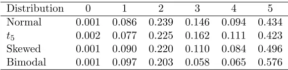
Within each of the simulation scenarios, nearly all subjects had at least one non-censored measurement, and approximately 90 percent had at least two non-censored observations. With the exception of the data generated from the bimodal random effects density (4) where 42.4 percent of subjects had at least one censored observation, a slight majority in each of the other scenarios had at least one censored observation. A complete description of the censoring pattern is given in Table 1.1.

Table 1.1: Proportion of subjects by number of non-censored observation for the four random effects densities considered in the simulations with q= 2 described in Section 1.5.

Distribution 0 1 2 3 4 5

Normal 0.001 0.086 0.239 0.146 0.094 0.434 t5 0.002 0.077 0.225 0.162 0.111 0.423 Skewed 0.001 0.090 0.220 0.110 0.084 0.496 Bimodal 0.001 0.097 0.203 0.058 0.065 0.576

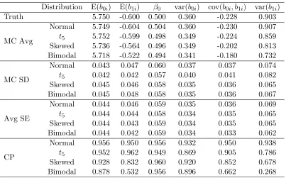
The simulation results are given in Table 1.2. When the random effects are correctly speci-fied, parameter estimators are unbiased, and the coverage probabilities attain their stated level of confidence. When the random effects have heavy tails (t5 distribution), parameter estima-tors are still unbiased although coverage probabilities for the covariance components do degrade slightly. Equation (1.4) suggests that the asymptotic bias in this scenario would be slight. When the random slope is slightly skewed, parameter estimators are biased, especially for E(b1i) (6.0

percent) and var(b1i) (−10.0 percent). Coverage probabilities for these parameters, in

particu-lar, are far from nominal. This illustrates that even slight departures from normality can lead to erroneous inference when the number of non-censored observations for each subject is small. In the case of severe misspecification with bimodal random slopes, the bias of all the parameter estimators increases in comparison to that under skewed random effects; the bias in the estima-tors for E(b1i) and var(b1i) is substantial (13.0 and −18.9 percent, respectively) and coverage

probabilities for these parameters are poor.

We also examined the effect of adding design points where there was unlikely to be any censoring and where censoring was likely. We generated 500 data sets with bimodal random effects where ti = (0,1,2,3,3.5,4,4.5)T ≡ tB and ti = (−2,−1,0,1,2,3,4)T ≡ tC for all

subjects. With measurements at tij = −2 and tij = −1, 99.9 and 90.5 percent of subjects

(29)

Table 1.2: Simulation results when Gaussian random effects were assumed for all models re-gardless of the true distribution of the random effects. The simulation included 500 data sets with 500 subjects each. MC Avg: Monte Carlo average of the parameter estimates; MC SD: Monte Carlo standard deviation of the parameter estimates; Avg SE: Average of the standard error estimates; CP: Monte Carlo coverage probability of the 95 percent Wald-type confidence intervals.

Distribution E(b0i) E(b1i) β0 var(b0i) cov(b0i, b1i) var(b1i)

Truth 5.750 -0.600 0.500 0.360 -0.228 0.903

MC Avg

Normal 5.749 -0.604 0.504 0.360 -0.230 0.907 t5 5.752 -0.599 0.498 0.349 -0.224 0.859 Skewed 5.736 -0.564 0.496 0.349 -0.202 0.813 Bimodal 5.718 -0.522 0.494 0.341 -0.180 0.732

MC SD

Avg SE

CP

from 21.8 percent. A more thorough description of the censoring pattern is given in Table 1.3. The simulation results for when ti = tA, tB, tC with bimodal random effects are shown

in Table 1.4. When there are more design points where censored observations are unlikely, bias is mitigated substantially and coverage probabilities improve, which is consistent with the asymptotic results in Section 1.2. Conversely, increasing the number of design points where censoring is likely has little effect on parameter estimation, illustrating that the overall censoring level has little to do with the bias.

(30)

Table 1.3: Proportion of subjects by number of non-censored observation when the true random effects density was bimodal and the time points where data were collected was varied. tA =

(0,1,2,3,4)T;tB= (0,1,2,3,3.5,4,4.5)T;tC = (−2,−1,0,1,2,3,4)T.

Time Points 0 1 2 3 4 5 6 7

tA 0.001 0.097 0.203 0.058 0.065 0.576 0.000 0.000

tB 0.001 0.096 0.203 0.049 0.029 0.033 0.052 0.538

tC 0.000 0.000 0.001 0.096 0.205 0.066 0.091 0.541

points centered at the empirical Bayes estimates ofbi derived from assuming Gaussian random

effects and with the number of quadrature points selected with a stated tolerance of 10−4. Dual-quasi Newton was used for optimization. 500 Monte Carlo data sets were generated for each scenario. To obtain starting values, the log likelihood was evaluated over a grid of ξ of 50 points for K = 1 and 150 points for K = 2 with starting values for β and σ2 set to the true values and for µand r set to the values that would give the true values for E(bi) and var(bi).

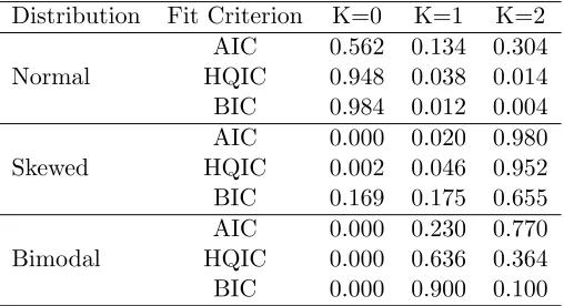
Table 1.5 gives the proportion of data sets that selected K = 0, 1, and 2 by several in-formation criterion. When the random effects are normally distributed, HQIC selects K = 0 for 94.8 percent of the data sets. However, when the random effects density was skewed and bimodal,K = 0 was selected only 0.2 and 0.0 percent of the time, respectively, andK= 2 was selected for 95.2 and 36.4 percent of the data sets, respectively. This illustrates that even with a modest sample size and loss of information due to censoring, the method is able to detect slight departures from normality while not over-fitting models where the true random effects density is Gaussian.

The results of the SNP parameter estimates when K was selected by HQIC are shown in Table 1.6. The SNP estimators when the random effects are not normally distributed are less biased than the estimators when Gaussian random effects were assumed. When the random effects were skewed, the bias for E(b1i) and var(b1i) is reduced to 0.5 and −0.3 percent,

(31)

Table 1.4: Simulation results when Gaussian random effects were assumed for the bimodal random effects but ti in (1.2) was varied. The simulation included 500 data sets with 500

subjects each. tA= (0,1,2,3,4)T; tB = (0,1,2,3,3.5,4,4.5)T; tC = (−2,−1,0,1,2,3,4)T; MC

Avg: Monte Carlo average of the parameter estimates; MC SD: Monte Carlo standard deviation of the parameter estimates; Avg SE: Average of the standard error estimates; CP: Monte Carlo coverage probability of the 95 percent Wald-type confidence intervals.

Time Points E(b0i) E(b1i) β0 var(b0i) cov(b0i, b1i) var(b1i)

Truth 5.750 -0.600 0.500 0.360 -0.228 0.903

MC Avg

tA 5.718 -0.522 0.494 0.341 -0.180 0.732

tB 5.715 -0.520 0.496 0.337 -0.175 0.722

tC 5.757 -0.590 0.500 0.360 -0.234 0.886

MC SD

tA 0.045 0.048 0.058 0.035 0.036 0.067

tB 0.046 0.048 0.059 0.033 0.034 0.066

tC 0.040 0.044 0.054 0.027 0.029 0.049

Avg SE

tA 0.044 0.042 0.059 0.034 0.033 0.062

tB 0.043 0.041 0.058 0.032 0.032 0.061

tC 0.039 0.043 0.053 0.026 0.030 0.058

CP

tA 0.878 0.532 0.956 0.896 0.662 0.268

tB 0.864 0.474 0.950 0.864 0.586 0.212

(32)

Table 1.5: Proportion of timeKwas selected using AIC, HQIC, and BIC when the SNP density was used to model the random effects density. The simulation included 500 data sets with 500 subjects each.

Distribution Fit Criterion K=0 K=1 K=2

Normal

AIC 0.562 0.134 0.304 HQIC 0.948 0.038 0.014 BIC 0.984 0.012 0.004

Skewed

AIC 0.000 0.020 0.980 HQIC 0.002 0.046 0.952 BIC 0.169 0.175 0.655

Bimodal

AIC 0.000 0.230 0.770 HQIC 0.000 0.636 0.364 BIC 0.000 0.900 0.100

1.6

Application

We now illustrate the proposed methods using data from 811 subjects in the IDEAL study with the CT genotype at polymorphic site upstream of interleukin (IL) 28B which is associated with virologic response (Thompson et al., 2010).

Subjects had viral load measurements taken at baseline and at 2, 4, and 12 weeks after treatment began, some of which were censored at the lower limit of quantification of 1.431 log₁₀ IU/mL. As shown in Figure 1.1, the viral load change over the first 12 weeks within-subject can be well approximated by a linear trajectory, and the measurement error and biological fluctuations at each time point can be assumed reasonably to be independent and Gaussian. However, standard therapy is not effective for all subjects, so the assumption that the subject-specific slopes are normally distributed is questionable.

Based on these observations, we consider the semiparametric model

Yij =b0i+b1itij+ij, (1.10)

where Yij is the log10 viral load for patient i at the jth time; tij is the time in weeks since

starting treatment; xij is null; sij = (1, tij)T; ij iid

∼ N(0, σ2); and bi = (b0i, b1i)T is the vector

of subject-specific intercept and slope, which we assume can be written as bi =µ+RZi with

Zi = (Z0i, Z1i)T,µ = (µ1, µ2)T, and R a (2×2) lower triangular matrix. We assume that Zi

follows the density (1.5) for the K described below. We do not observeYij but instead observe

Qij with lij ≡1.431.

(33)

Table 1.6: Simulation results when the SNP density was used to model the random effects density. Models with K= 0, K = 1, andK = 2 were fit and K was selected using HQIC. The simulation included 500 data sets with 500 subjects each. MC Avg: Monte Carlo average of the parameter estimates; MC SD: Monte Carlo standard deviation of the parameter estimates; Avg SE: Average of the standard error estimates; Ratio MSE: Ratio of the Monte Carlo mean square error between K= 0 and K selected by the HQIC.

Distribution E(b0i) E(b1i) β0 var(b0i) cov(b0i, b1i) var(b1i)

Truth 5.750 -0.600 0.500 0.360 -0.228 0.903

MC Avg

Normal 5.749 -0.603 0.504 0.358 -0.229 0.905 Skewed 5.750 -0.598 0.496 0.358 -0.227 0.900 Bimodal 5.747 -0.590 0.496 0.360 -0.222 0.878

MC SD

Normal 0.043 0.047 0.060 0.040 0.038 0.077 Skewed 0.046 0.050 0.060 0.044 0.041 0.090 Bimodal 0.045 0.048 0.058 0.037 0.039 0.080

Avg SE

CP

Ratio MSE

(34)

uncensored. Still, 12.8 percent of patients only have one or two non-censored measurements. At week 12, 35.2 percent of subjects’ responses are censored. The proportion of observations that were censored at each time point and the proportion of subjects by number of uncensored measurements are given in Tables 1.7 and 1.8, respectively.

Table 1.7: Proportion of responses censored at each time point for the 811 patients with CT genotype in the IDEAL trial.

Time (weeks) 0 2 4 12 Overall

Proportion 0.000 0.020 0.053 0.352 0.105

Table 1.8: Proportion of subjects by number of uncensored viral load measurements for the 811 patients with the CT genotype in the IDEAL trial.

Uncensored Measurements 1 2 3 4

Proportion 0.045 0.083 0.312 0.551

The fit statistics and relevant parameter estimates from fitting model (1.10) with K = 0, K = 1, andK= 2 appear in Table 1.9. While most of the parameter estimates are only altered marginally as K increases, the estimate for E(b1i), the average weekly log viral load decline,

changes substantially. When K = 1 and K = 2 the estimate is more than one standard error away from the estimate whenK = 0.

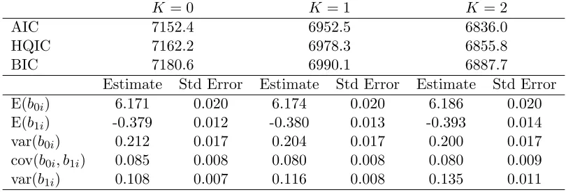
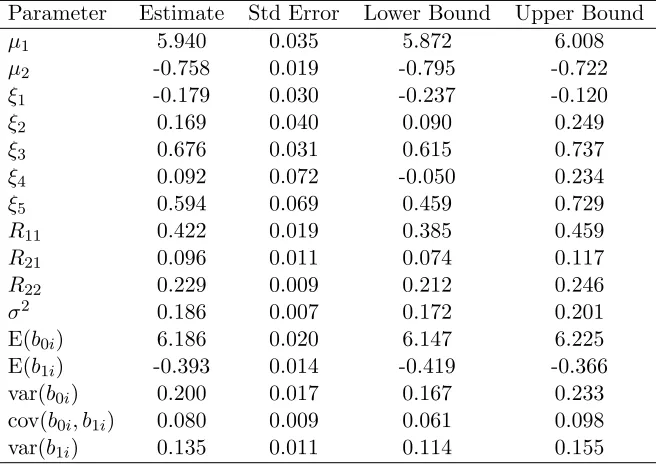
Each of the information criteria preferred K = 2, so we present the density estimates from that model in Figure 1.5 and parameter estimates for the nuisance parameters in Table 1.10. The contour plot for the bivariate random effects shows the presence of two or possibly three modes. SNP density estimation frequently results in a spurious mode to capture mass in what is actually a long tail, so one should be cautious about over-interpreting this third mode. The marginal density estimates show a large departure from normality for the subject specific slope, confirming our prior hypothesis, but little departure from normality in the baseline log₁₀ viral load. The majority of patients with the CT genotype experience very modest weekly viral load changes around -0.25 log₁₀ IU/mL/week. However, the remaining patients experience greater viral load decline with the mode at approximately -0.85 log₁₀ IU/mL/week.

(35)

Table 1.9: Information criteria and parameter estimates from fitting model (1.10) concerning the IDEAL study withK = 0,K = 1, andK = 2

K= 0 K = 1 K= 2

AIC 7152.4 6952.5 6836.0

HQIC 7162.2 6978.3 6855.8

BIC 7180.6 6990.1 6887.7

Estimate Std Error Estimate Std Error Estimate Std Error

E(b0i) 6.171 0.020 6.174 0.020 6.186 0.020

E(b1i) -0.379 0.012 -0.380 0.013 -0.393 0.014

var(b0i) 0.212 0.017 0.204 0.017 0.200 0.017

cov(b0i, b1i) 0.085 0.008 0.080 0.008 0.080 0.009

var(b1i) 0.108 0.007 0.116 0.008 0.135 0.011

respond to standard therapy while the majority with the CT genotype do not show substantial improvement. The IL28B genotype has been shown to be a strong predictor of virological response for HCV-infected patients undergoing standard therapy. However, the analysis here suggests that, even within this genotype, there are responders and non-responders, and more research is required to determine why patients respond to therapy. This example illustrates that fitting a flexible model for the random effects when the response is censored can not only substantially alter the estimates of clinically relevant parameters like E(b1i) but can also lead to

a fuller understanding of the underlying process. Given the multi-modality of the subject-specific slopes, some would even question if E(b1i) is a useful parameter with which to characterize the

population.

1.7

Discussion

(36)

Table 1.10: Parameter estimates, standard errors, and a 95 percent Wald-type confidence limits from fitting model (1.10) assuming the random effects followed the SNP density with K= 2.

Parameter Estimate Std Error Lower Bound Upper Bound

µ1 5.940 0.035 5.872 6.008

µ2 -0.758 0.019 -0.795 -0.722

ξ1 -0.179 0.030 -0.237 -0.120

ξ2 0.169 0.040 0.090 0.249

ξ3 0.676 0.031 0.615 0.737

ξ4 0.092 0.072 -0.050 0.234

ξ5 0.594 0.069 0.459 0.729

R11 0.422 0.019 0.385 0.459

R21 0.096 0.011 0.074 0.117

R22 0.229 0.009 0.212 0.246

σ2 0.186 0.007 0.172 0.201

E(b0i) 6.186 0.020 6.147 6.225

E(b1i) -0.393 0.014 -0.419 -0.366

var(b0i) 0.200 0.017 0.167 0.233

cov(b0i, b1i) 0.080 0.009 0.061 0.098

var(b1i) 0.135 0.011 0.114 0.155

are Gaussian, we recommend using the SNP density for censored longitudinal data when the number of non-censored observations is small to avoid erroneous inference. More specifically, we suggest fitting SNP models for severalKto determine if the random effects density deviates from normality. Visual inspection of the estimated densities for each K >0 as well as information criteria can be used to assess if the random effects density is non-normal. When the random effects distribution deviates from normality, the information criteria rarely select K = 0 even with modest sample sizes, indicating the method’s ability to detect non-normal distributions. In addition to improved inference, one gains insight into the data generating process if a flexible random effects model is used.

Within the economics literature, there has been substantial work on developing tests to determine if the error distribution is Gaussian in censored regression models with independent responses. Future work could extend those tests to random effects densities.

(37)

0.00 0.05 0.10 0.15 0.20 0.25 0.30 0.35

4.0 4.5 5.0 5.5 6.0 6.5 7.0 −3

−2 −1 0 1

Skewed Random Effects

Random Intercept Random Slope 0.0 0.1 0.2 0.3 0.4 0.5

4.0 4.5 5.0 5.5 6.0 6.5 7.0 −3

−2 −1 0 1

Bimodal Random Effects

Random Intercept

Random Slope

Figure 1.2: Contour plot of the true random effects densities from the “skewed” and “bimodal” scenarios considered in the simulation described in Section 1.5. In each case, the densities were a 70-30 mixture of two normals.

0.00 0.05 0.10 0.15 0.20 0.25 0.30 −3 −2 −1 0 1

4 5 6 7

Average Contour Plot

Random Intercept

Random Slope

4.0 5.0 6.0 7.0

0.0 0.1 0.2 0.3 0.4 0.5 0.6

Marginal Density of Intercept

Random Intercept

Density

−3 −2 −1 0 1

0.0 0.1 0.2 0.3 0.4 0.5

Marginal Density of Slope

Random Slope

Density

(38)

0.0 0.1 0.2 0.3 0.4 0.5

−3 −2 −1 0 1

4 5 6 7

Average Contour Plot

Random Intercept

Random Slope

4.0 5.0 6.0 7.0

0.0

0.1

0.2

0.3

0.4

0.5

0.6

Random Intercept

Density

−3 −2 −1 0 1

0.0

0.1

0.2

0.3

0.4

0.5

0.6

0.7

Random Slope

Density

(39)

0.0 0.5 1.0 1.5 2.0

5.0 5.5 6.0 6.5 7.0 −1.5

−1.0 −0.5 0.0

Contour Plot of Random Effects

Random Intercept

Random Slope

5.0 5.5 6.0 6.5 7.0 7.5

0.0

0.2

0.4

0.6

0.8

Random Intercept

Density

−2.0 −1.5 −1.0 −0.5 0.0 0.5

0.0

0.5

1.0

1.5

2.0

Random Slope

Density

(40)

Chapter 2

Assessing the Effect of Organ

Transplantation on the Distribution

of Residual Lifetime

2.1

Introduction

Lung transplantation remains the definitive therapy for many end-stage lung diseases including chronic obstructive pulmonary disorder (COPD), cystic fibrosis (CF), and idiopathic pulmonary fibrosis (IPF) (Kotloff and Thabut, 2011). In comparison to other solid organ transplantations, unadjusted one- and three-year survival rates after primary lung transplantation remain poor, 83.8 and 63.2 percent, respectively, (based on Organ Procurement and Transplantation Network data as of March 30, 2012). Despite poor post-transplant survival rates, the number of lung transplantations performed in the United States grew from 959 in 2000 to 1,770 in 2010. Lung transplantation remains controversial, in part due to the intensive use of health care resources, high cost, and relative uncertainty regarding survival and quality of life benefit.

A definitive understanding of the survival benefit of transplantation in a national cohort is needed to improve organ allocation and justify the large health care resources needed for transplantation. Specifically, we want to compare how the distribution of residual lifetime if a patient were to undergo a transplant compares to the distribution of the residual lifetime had the patient, possibly contrary to fact, never been transplanted. That is, we seek to quantify the survival benefit or loss of transplantation from a causal perspective.

(41)

examined the survival benefit of transplantation for COPD patients; Aurora et al. (1999); Liou et al. (2001); Aigner et al. (2004); Liou et al. (2006, 2007); Liou and Cahill (2008) for CF patients, including pediatric patients; and Thabut et al. (2003) for IPF patients. More comprehensive studies on the efficacy of transplantation, including Hosenpud et al. (1998); DeMeester et al. (2001); Charman et al. (2002) have examined the effect of transplantation using data prior to the implementation of the lung allocation score (LAS) in 2005. These older studies may not represent the current effectiveness of transplantation or medical management and cannot examine the relationship between survival benefit and LAS, a clinically meaningful priority score described subsequently in detail. In one of the few studies on the survival benefit of transplantation in the LAS era, Russo et al. (2011) found that the survival benefit generally increased with increasing LAS, but this study did not incorporate other important factors possibly related to survival benefit including native disease.

Most of the research cited above has used a proportional hazard model with a time-dependent covariate for transplantation to quantify the effect of transplantation. This method-ological approach implicitly assumes that transplantation, that is, movement from the waitlist group to the post-transplant group, is independent of prognosis. Other methodological ap-proaches used to assess the survival benefit of transplantation in the clinical literature have also made this assumption (for example Thabut et al., 2008; Russo et al., 2011). While con-venient analytically, this assumption ignores how organs are allocated in the United States, and this limitation has been explicitly acknowledged in the clinical literature (Liou and Cahill, 2008; Thabut and Fournier, 2009). The lack of a comprehensive study of the survival benefit of lung transplantation using methodology with clinically reasonable assumptions has motivated the development of causal methods for transplantation.

To understand the methodological challenges of this problem, it is imperative to conceptu-alize how treatment, organ transplantation here, is assigned and how this treatment assignment differs from that in most observational studies. Because the number of patients needing a lung transplant exceeds the number of organs available, the Organ Procurement and Transplanta-tion Network (OPTN) maintains a naTransplanta-tional waiting list to offer in an orderly way available organs to patients. Across all solid organ transplants, patients with worse waitlist prognosis are given preference when an organ becomes available. Since 2005, the lung allocation score (LAS) has been used to prioritize patients on the waitlist for lung transplantation (Egan and Kotloff, 2005). LAS is a composite score, ranging from 0 to 100, comprised of over a dozen patient char-acteristics and lab values that predict waitlist mortality and post-transplant survival. Higher LAS values indicate a higher priority for transplantation and worse waitlist prognosis.

(42)

studies. Robins and colleagues propose three general methods to obtain valid causal inference of treatment in the presence of confounders: G-computation (Robins, 1986); marginal struc-tural models, typically estimated using inverse probability of treatment weighted estimators (Hern´an et al., 2000; Robins et al., 2000); and structural nested failure time models, estimated by G-estimation (Robins, 1989; Robins et al., 1992; Robins, 1992, 2005). Structural nested failure time models estimated using G-estimation do not suffer from the null paradox, unlike G-computation, and unlike marginal structural models allow direct modeling of the interac-tion between covariates and treatment and avoid some of the instability associated with inverse weighting. Given the advantages, we considered structural nested transformation models for our analysis. We note that our approach differs from the proportional hazard models considered by Schaubel et al. (2006, 2009) in their methodological work on the survival benefit of liver transplantation. Other distinctions between our work and the work of Schaubel et al. (2006, 2009) are discussed later.

(43)

In Section 2.2, we develop the problem using a potential outcome framework and describe the notation for the observed data. In addition, we introduce a model for organ assignment and a structural nested failure time model to relate the residual lifetime distribution if a patient were transplanted to the distribution if she were never transplanted. In Section 2.3, we describe a class of estimators for parameters in our structural nested failure time model, derive the asymptotic properties of the class, and discuss reasonably efficient estimators within the class. Section 2.4 gives computational strategies to mitigate the problems typically encountered with censored failure times. Section 2.5 describes the results of a simulation study. In Section 2.6, we demonstrate our method on the survival benefit of lung transplantation using data from the United Network for Organ Sharing (UNOS). We conclude in Section 2.7.

2.2

Developing a Statistical Framework

2.2.1 Potential Outcome Framework

We consider a hypothetical population of subjects that are eligible for organ transplantation. At the patient level, we denote time 0 to be the time that the patient was first listed on the waitlist. LetT∗(∞) be the potential time from listing until death for a randomly selected individual in the population assuming that the patient never received an organ transplantation. For many organs, there are differences in the characteristics of the donor organ that are clinically relevant. We denote by Q a random vector of donor organ characteristics. We define T∗(t, q) to be the survival time for a random patient awaiting organ transplantation had she been transplantedt days after entering the waitlist with donor organ characteristics Q=q assuming that she had not already received an organ and was alive on the waitlisttdays after being listed. AsT∗(∞) andT∗(t, q) may not be observed on a random subject, these are known as potential outcomes. Define X∗(t) to be the history of time-dependent covariates through t days after listing assuming the patient had not been transplanted and had not died prior to time t. The history of time-dependent covariates are also potential outcomes. Typically, covariates are not measured after the patient has been transplanted, so it is not useful to consider potential covariate values after transplantation.

If we let Q be the set of all possible donor organ characteristics, then we can define the set of all potential outcomes for subjectias

P_i=hT_i∗(∞),{T_i∗(t, q), t≤T_i∗(∞), q∈ Q},{X∗_i(t), t≤T_i∗(∞)}i.

(44)

only meaningful and defined if the patient would have survived on the waitlist for t days or, symbolically, T∗(∞)≥t.

2.2.2 Failure Time Model

The goal of determining the effect of transplantation on residual lifetime can now be character-iz