Advances in Nonparametric Bayesian Methods for Clustering and Classification.

(1)

ABSTRACT

KAO, YIMIN. Advances in Nonparametric Bayesian Methods for Clustering and Classification. (Under the direction of Brian J. Reich.)

Nonparametric Bayesian methods have proven to be extremely useful due to their flexibility and applicability to a wide range of problems. In this thesis, several non-parametric Bayesian techniques are presented for classification and clustering. The first chapter is motivated by a computer security problem, and a nonparametric Bayesian model is proposed by implementing the Dirichlet process mixture (DPM) prior for classi-fying programs as benign or malicious and simultaneously clustering malicious programs. The novelty of the model is using this clustering algorithm to improve the classification accuracy. In an analysis of malicious and benign programs obtained from Los Alamos National Lab, the DPM model gives better classification performance than the elastic net logistic (ENL) model, and is competitive with the support vector machine (SVM). More importantly, the DPM model identifies clusters of programs during the classification procedure which is useful for reverse engineering.

In the second Chapter, we propose a new method for the fundamental task of testing for dependence between two groups of variables. The response densities under the null hypothesis of independence and the alternative hypothesis of dependence are specified by nonparametric Bayesian models. Under the null hypothesis, the joint distribution is modeled by the product of two independent DPM priors; under the alternative, the full joint density is modeled by a DPM prior. The test is then based on the posterior probability of favoring the alternative hypothesis. The proposed test not only has good performance for testing linear dependence among other popular nonparametric tests, but is also preferred to other methods in testing many of the nonlinear dependencies we explored.

(2)

c

(3)

Advances in Nonparametric Bayesian Methods for Clustering and Classification

by Yimin Kao

A dissertation submitted to the Graduate Faculty of North Carolina State University

in partial fulfillment of the requirements for the Degree of

Doctor of Philosophy

Statistics

Raleigh, North Carolina

2014

APPROVED BY:

Howard D. Bondell Sujit Ghosh

Yichao Wu Grady Miller

Brian J. Reich

(4)

BIOGRAPHY

(5)

ACKNOWLEDGEMENTS

First, I want to express my great appreciation to my advisor Dr. Brian Reich. His profound knowledge of statistics benefits my journey of pursing professional knowledge. More importantly, his passion and patience both influence my attitude towards research. I feel extremely thankful to work with my advisor.

I also want to take this opportunity to thank Dr. Curtis Storlie for co-advising the first chapter of my thesis and Dr. Howard Bondell for co-advising the second and third chapters of my thesis. Also, I want to thank Dr. Sujit Ghosh and Dr. Yichao Wu for joining my committee and giving me many suggestions on my work.

Finally, I want to thank to my family and friends who always give me support and understanding.

“A dream doesn’t become reality through magic; it takes sweat, determination and hard

(6)

LIST OF TABLES

Table 2.1 Seven scenarios in the simulation study. . . 15 Table 2.2 FDR, Power, and AUC subscripted with standard errors for the ENL,

SVM and DPM models under seven scenarios. The Wilcoxon signed-rank test for the pairwise differences of the ENL, SVM and DPM models under Power, and AUC are all significant. . . 16 Table 2.3 Overall TPC and FPC subscripted with standard errors for scenario

2-7. (∗represents the Wilcoxon signed-rank test for the pairwise differ-ences of spectral clustering method and DPM models are shown to be significant, p-value <0.05. No ∗ represents non-significant.) . . . 17 Table 2.4 FDR, Power, and AUC subscripted with standard errors for the ENL,

SVM, and the DPM models with {(K0, K1) = (150,200)}. . . 19

Table 2.5 Clustering results for 5 testing malicious programs (ID:4, 87, 252, 342, 972), each lists the top 5 training samples ID with highest pairwise clustering probabilities in the parenthesis. . . 21

Table 3.1 Hyperparameters (a, b) under different sample sizesn. . . 29 Table 3.2 Power of each test (columns) for each simulation settings and sample

sizen (rows). A∗indicates that the power is significantly different than the power of DPM test. . . 35 Table 3.3 Numbers of rejections (of theN = 4371 tests), and Cohen’sκ statistics

for each pair of methods. . . 36

Table 4.1 Posterior probabilities of pairwise associations. . . 51 Table 4.2 10-fold cross validation of deviances for the independent DPM (I), joint

(10)

LIST OF FIGURES

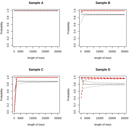
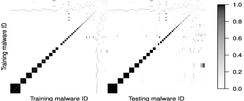
Figure 2.1 P(ξs∗ = 1 | Z_s∗,Z) of the ENL (black lines) and the DPM models (red lines) under different lengths of traces for 4 malware samples. . . 22 Figure 2.2 Overall clustering heat map for ordered training and testing malware

with (K0, K1) = (150,200) . . . 23

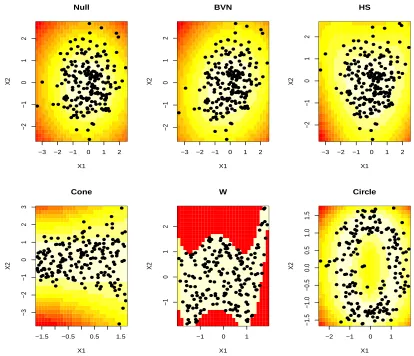
Figure 3.1 True log density (background color) and one simulated data set (points) for each simulation design. . . 33 Figure 3.2 Six pairs of genes where there are disagreements among the tests. The

red lines are the linear fitted lines. . . 37

Figure 4.1 KLD under high-dimensional data. . . 47 Figure 4.2 Factorization probability (that is, the posterior probability that each

pair of variables are in the same cluster) plots for four simulated data sets. . . 48 Figure 4.3 Tracks of 79 tropical storm tracks after year 2005. . . 49 Figure 4.4 Pairwise scatter plots for the tropical storm track data. . . 50 Figure 4.5 Factorization probability plot of the 344 tropical storm tracks . . . . 51 Figure 4.6 Estimated density function of initial (left) and final (right) spatial

locations. . . 52 Figure 4.7 Estimated conditional density function of the final location given the

initial spatial location (denoted as a solid triangle). . . 54 Figure 4.8 2-dimensional data with b = 0,0.3,0.5,0.8. Panel (a) plots the KLD

for the 100 simulated data sets, and Panel (b) plots the posterior prob-abilities of the true factorization under the RJ model for the 100 data sets. . . 55 Figure 4.9 3-dimensional data with b = 0,0.3,0.5,0.8. Panel (a) plots the KLD

for the 100 simulated data sets, and Panel (b) plots the posterior prob-abilities of the true factorization under the RJ model for the 100 data sets. . . 55 Figure 4.10 4-dimensional data with b = 0,0.3,0.5,0.8. Panel (a) plots the KLD

(11)

Chapter 1

Introduction

Nonparametric Bayesian models have been widely used in many applications due to their flexibility and applicability. In this thesis, several nonparametric Bayesian tech-niques are presented for classification and clustering. The new method is motivated by a computer security problem which requires statistical methods to quickly and accurately flag malicious programs. We propose a nonparametric Bayesian approach by implement-ing the Dirichlet process mixture (DPM) model for classifyimplement-ing programs as benign or malicious, and simultaneously clustering malicious programs (Chapter 2). The novelty of the model is using this clustering algorithm to improve the classification accuracy. The simulation study shows that the DPM model outperforms the elastic net logistic (ENL) regression and the support vector machine (SVM) in classification performance under most of the scenarios we considered, and also outperforms the spectral clustering method for grouping similar malware. In an analysis of malicious and benign programs obtained from the Los Alamos National Lab, the DPM model gives better classification perfor-mance than the ENL model, and is competitive with the SVM method. More importantly, the DPM model identifies clusters of programs during the classification procedure which is useful for reverse engineering.

(12)

of favoring the alternative hypothesis. The proposed test not only has good performance for testing linear dependence, but is also preferred to other methods in testing many of the nonlinear dependencies we explored. In the analysis of the gene expression data, we compare different methods for testing pairwise dependence between genes. The proposed test identified some dependent structures that are not detected by other methods.

(13)

Chapter 2

Malware detection using

nonparametric Bayesian clustering

and classification techniques

2.1

Introduction

Malware is a term used to describe a variety of forms of hostile, intrusive, or annoying software or program code. It was recently estimated that 30% of computers operating in the US are infected with malware (PandaLabs, 2012). More than 286 million unique variants of malware were detected in 2010 alone (Symantec, 2011), and it is widely be-lieved that the release rate of malicious programs is now far exceeding that of legitimate program applications (Symantec, 2008). The cost incurred by US companies due to mal-ware was estimated in 2011 to be $338 Billion/year (Consumer Reports 2011). A large majority of new malware is created through simple modifications to existing malicious programs or by using code obfuscation techniques such as a packer (Royal et al., 2006). A packer compresses a program much the same way a compressor like Pkzip does, and then attaches its own decryption/loading stub which unpacks the program before resuming execution normally at the programs original entry point.

(14)

eventually works its way into the database, which can take weeks or even longer. There are two methods for antivirus scanners to implement their technology. The first is via a static signature scanning method, which uses a sequence of known bytes in a program and tests for the existence of this sequence. The second is using heuristic detection tech-nologies which are intended to protect against zero-day (i.e., new) malware and malware not in the signature database.

Because of the signature-based susceptibility to new malware, classification proce-dures based on statistical and machine learning techniques have been employed with varied success to make a decision about the integrity of an unknown program (Reddy et al., 2006; Reddy and Pujari, 2006; Stolfo et al., 2005; Dai et al., 2009). These methods have generally revolved around n-gram analysis of the static binary or dynamic trace of the malicious program. Recently, some promising results have come from a Markov chain representation of the program trace (Anderson et al., 2011; Storlie et al., 2013). In these works, dynamic traces from many samples of malware and benign programs were used to train a classifier. A dynamic trace is a record of the sequence of instructions executed by the program as it is actually running. Although some success has been achieved using disassembled static binary files, this cannot always be done, particularly if the program uses an unknown packer, and therefore this approach has similar shortcomings to the signature based methods.

The classification of malware is a very important problem by itself, but it is only the beginning of malware analysis. Once malware is discovered on a host in an enterprise network, for example, the time consuming process of reverse engineering (RE) (Chikof-sky and Cross, 1990) commences. A highly trained cyber professional can spend a day to weeks uncovering the purpose of the malware, its sender, and the extent of the attack. Not only does this tedious process require substantial time and labor, but it also results in a slower response. An organization cannot adequately respond to a malware infection until they understand what it does.

(15)

dimensionality required to adequately represent a computer program. Previous work that addresses the malware clustering problem relies on spectral clustering techniques (An-derson et al., 2012) and other heuristic approaches (Storlie et al., 2013).

The proposed model in this chapter builds upon the work of Anderson et al. (2011) and Storlie et al. (2013) by explicitly modeling the dynamic trace (DT) data as a Markov chain. Unlike the previous works, a rigorous probabilistic model is established for the generation of a program trace. Specifically, the nonparametric Bayesian model (Ghosh and Ramamoorthi, 2003) accomplishes both clustering and classification via discrimi-nant analysis. This general approach has been applied successfully in density estimation problems (MacEachern, 1994; Escobar, 1994; West et al., 1994; Escobar and West, 1995; Muller and Quintana, 2004; Dunson, 2010), and also for classification and clustering purposes (Jackson et al., 2007; Shahbaba and Neal, 2009; Davy and Tourneret, 2010; Zhu et al., 2012). The contribution of this chapter is to tailor this general approach to malware detection, and to illustrate that this approach has benefits compared to current approaches to this problem. The DTs are assumed to be Markovian, which has been demonstrated to be a reasonable approximation in previous work (Storlie et al., 2013), and thus the proposed model focuses on the transition probability matrix. To perform the classification of the programs, the proposed method fits separate models for the dis-tributions of transition matrices for malware and benign programs. To ensure that the model is flexible enough to capture the complexities of DTs, the Dirichlet process mix-ture (DPM) (Antoniak, 1974) prior is applied to span the entire space of row-stochastic matrices. After fitting the models using the training data, it classifies programs based on the posterior probability of being a malware in a way that controls the Bayesian false discovery rate. A natural by-product of the DPM model is that it places programs into clusters. Therefore, in addition to classification, the proposed model simultaneously ob-tains Monte Carlo estimates of the probability that a new program clusters with each malware in the training set, which can be used to aid reverse engineering.

(16)

chapter.

2.2

Statistical model for malware detection

2.2.1

Description of dynamic trace data

A dynamic trace (DT) is a sequence of processor instructions called during execution. Let N be the total number of programs in the sample indexed by s, s = 1, ..., N. The dynamic trace of the sth program is denoted as {Ys1, ..., YsNs}, where Yst ∈ {1, ..., M} is

the tth instruction called during execution, Ns is the length of the dynamic trace, and

M is the number of classes of processor instructions. As Storlie et al. (2013), we treat similar instructions as identical, by grouping similar instructions together into one ofM classes. Given the first-order Markov structure, it is sufficient to specify the distribution of the first instructionYs1 and the distribution of theM×M transition matrixZs, where the (r, c) component, r, c∈ {1, ..., M}, of the Zs is the count

Zsrc = Ns

X

t=2

I(Yst−1 =r, Yst =c).

Both the initial instruction distribution and the transition matrix distribution are allowed to vary by programs. The initial instruction of a program s has distribution

P(Ys1 = j) = qsj, with PM_j₌₁qsj = 1. The subsequent instructions, t = 2, ..., Ns, are modeled as P(Yst = c| Yst−1 = r) = Psrc, with PM_c₌₁Psrc = 1, for all r. Ps is the M ×

M matrix with (r, c) component Psrc which is the row-stochastic transition probability matrix for Zs.

BecauseNsis typically very large, the initial instructionYs1provides little information

about the characteristics of the DT. Therefore, Ys1 can be ignored and the sufficient

statistic for the DT is then the transition matrix Zs. The likelihood function for one single program s has a simple form

f(Zs | Ps) = M Y

r=1

M Y

c=1

PZsrc

(17)

The objective of this study is to focus entirely on the transition matrix Zs, and to build a flexible nonparametric Bayesian model for the distribution of Ps to capture variability across programs.

The remainder of this chapter only describes the model for the malicious programs to simplify notation. The model for benign programs is identical. Chapter 2.3 describes the full model including both benign and malicious programs. Given this full model, a new program can be classified as either benign or malicious, and also identify clusters of similar programs.

2.2.2

Prior for the transition probability matrix distribution

The transition probability matrix Ps for one single program s is assumed to have Ps

iid

∼ F for alls, whereF represents the distribution of transition probability matrices across malicious programs. In practice, there is only limited information about the form of the distribution before the data are observed. Therefore, rather than specify a particular parametric model, the proposed method places a prior on F to ensure enough flexibility to capture variability among the malicious programs.

A straightforward nonparametric Bayesian model is to assume F has a Dirichlet process prior (Ferguson, 1973)

Ps iid

∼ F (2.2)

F ∼ DP(α,Fb),

where α > 0 is the concentration parameter and Fb is the base distribution of the Dirichlet process prior; large α forces the prior of F closer to Fb, and vice versa. In our application, Fb is the Matrix Dirichlet (MD) distribution, Fb = MD(γP˜), which is centered on a constant M ×M matrix ˜P with a concentration scalar parameterγ > 0. This MD distribution implies that if an M ×M random matrix X is from MD(γP˜), then each row ofX independently follows theM-dimensional Dirichlet distribution with concentration parameters equal to the corresponding row of γP˜

Xr

iid

(18)

where Xr, ˜Pr are the rth row of X and ˜P respectively. In other words, ˜P controls the

general shape of the base distribution Fb, and γ controls the variance of Fb with large γ corresponding to smaller variance.

The Dirichlet process prior in (2.2) can be written as a mixture density (Ferguson, 1983)

f(Ps | w,λ) =

∞

X

k=1

wk·δ(Ps | λk), (2.3)

where λ = {λk : k = 1, ...,∞}, w ={wk :k = 1, ...,∞}, and the mixture probabilities

wk >0 satisfy P∞

k=1wk = 1, δ is the Dirac Delta density with point mass at Ps = λk,

and λk

iid

∼ Fb. Equation (2.3) can be thought of as mixing infinitely-many point mass distributions, and λk controls the shape of the kth point mass distribution.

While the Dirichlet process prior in (2.3) has attractive features, it is not appropriate for the analysis of transition probability matrices because it gives a discrete distribution. In other words, it implies that the transition probability matrices of two executable programs could be identical, which is unrealistic. Therefore, the proposed model considers a Dirichlet process mixture (DPM) prior (Antoniak, 1974; Neal, 2000) to alleviate this concern. The DPM prior has the form

Ps | θs, σ iid

∼ F = MD(σθs) (2.4)

θs iid

∼ G

G ∼ DP(α,Fb),

where the scalar parameter σ > 0 controls the variance of the distribution of Ps with large σ corresponding to smaller variance, theM ×M matrix θs is the shape parameter of the distribution of Ps, α and Fb are defined as in (2.2). Compared with (2.2), the distribution of Ps is now continuous as the MD distribution is continuous, and therefore the probability of two transition probability matrices are identical is zero. This DPM model can also be written as a mixture model density

f(Ps | w,λ, σ) =

∞

X

k=1

wk·fM D(Ps | σλk), (2.5)

(19)

Equation (2.5) is the stick-breaking representation of a DPM model (Ferguson, 1983). The weightswkare modeled in terms of latentvk ∼Beta(1, α). The first weight isw1 =v1.

The remaining elements are modeled as wk = vkQk

−1

j=1(1−vj), where

Qk−1

j=1(1−vj) =

1−Pk−1

j=1wj is the remaining probability after accounting firstk−1 mixture weights. By

construction, little is lost by truncating the sum at a large number of terms, sayK, where the last term vK is fixed to be 1, and thus

PK

k=1wk = 1. Accuracy of the approximation is monitored by inspecting the posterior of the final termwK which should be near zero if the approximation is sufficient.

2.2.3

Cluster indexes and marginalizing over the transition

prob-ability matrix

The mixing structure in (2.5) can also be viewed as a clustering model by introducing an auxiliary variablegs∈ {1, ..., K}to represent the cluster index ofsthmalware observation, wheregs=k indicatessth malware is in clusterk. The DPM model assumes that thePs of all the malware in the same cluster are from the same MD distribution, and the prior probability of a malware being in clusterk iswk. This representation facilitates Bayesian clustering in the hierarchical structure

f(Zs |Ps) = M Y

r=1

M Y

c=1

PZsrc

src (2.6)

Ps | λ, σ, gs=k iid

∼ MD(σλk) (2.7)

λk | γ

iid

∼ MD(γP˜) (2.8)

P(gs=k |w) = wk. (2.9)

The structure above includes the transition probability matrix Ps, however, Ps itself is not of interest and includingPsin the model will increase the computing time. Therefore, by marginalizing over Ps, the likelihood function of Zs can be derived as a Matrix Multivariate P´olya (MMP) distribution (derived in Appendix A.1)

(20)

Therefore, (2.6) and (2.7) are replaced by (2.10), which is the the hierarchical model used in the study. Similarly, (2.10) can be written as the mixture model density

f(Zs | λ, σ,w) = K X

k=1

wk·fM M P(Zs |λk, σ), (2.11)

where fM M P is the probability density function of MMP distribution.

2.3

Classification and clustering

This chapter describes how the DPM model classifies and clusters programs. First, the full model is specified which includes both benign and malicious programs. After the full model is defined, the Bayesian classification and clustering algorithms are described.

2.3.1

The full model

The full model is constructed by introducing another auxiliary variable ξs, where

ξs= (

1 if program s is malicious

0 if program s is benign (2.12)

and P(ξs = 1) =ψ is the prior probability of being a malicious program. The full model of a single program s can be written as

f(Zs | ξs =i,Θi) =

Ki

X

k=1

wik·fM M P(Zs | λik, σi), i= 0,1 (2.13) λik

iid

∼ MD(γiP˜i)

ξs ∼ Bern(ψ),

where Θ0 = {λ0, γ0, σ0,w0, K0} and Θ1 = {λ1, γ1, σ1,w1.K1} are the collections of

(21)

variance between clusters) are assigned to have non-informative gamma distributions. The hyperparameter of the stick breaking representation in (2.5) is αi ∼Gamma(ai, bi), where ai and bi are picked such that the prior on the number of clusters (i.e., number of unique values of gs) is fairly uninformative. More details of the model settings are in Appendix A.2.

2.3.2

Bayesian classification

Let Z be the collection of all observed Zs where ξs is known. The model is then trained by Z, and the posterior probability of a new program s∗ being a malware is

P(ξs∗ = 1 | Z_s∗,Z) (2.14)

= f(Zs∗ | ξs∗ = 1,Z)·P(ξs∗ = 1)

f(Zs∗ | ξ_s∗ = 1,Z)·P(ξ_s∗ = 1) +f(Z_s∗ | ξ_s∗ = 0,Z)·P(ξ_s∗ = 0)

.

Under the Bayes rule, the new program s∗ is classified as malicious if this probability exceeds a predefined threshold.

Let Us∗ denote the approximation of the posterior probability of being a malware calculated by post processing the MCMC samples (described in Appendix A.3)

Us∗ =

PnM

l=1f(Zs∗ | Θ1 (l)

,Z) PnM

l=1f(Zs∗ | Θ1

(l)_,_Z_{) +}PnM

l=1f(Zs∗ | Θ0

(l)_,_Z₎, (2.15)

where Θi(l) is the collection of parameters in the lth MCMC step under class i (i = 1

for malicious, i = 0 for benign program), and nM is the number of MCMC iterations. The classification is to label program s as malicious if Us∗ > T, where T is a tuning threshold. One way to determine the thresholdT is by using the Bayesian false discovery rate (BFDR) control procedure (Efron and Tibshirani, 2002; Newton et al., 2004; Storey et al., 2004; Muller et al., 2006) under the observed samples, which is described below:

1. Suppose there arenZ observed programs. Define BFDR under thresholdt as

BFDRt = PnZ

s=1rs(1−Us)

PnZ s=1rs

, where rs =I(Us > t). (2.16)

In practice, to avoid PnZ

s=1rsbeing too small (only very few programs are classified as

malicious),t is restricted to satisfyt :PnZ

(22)

number. In this chapter, R0 is set to be 5.

2. Let U_h(1) < U_h(2) < ... < U_h(nZ) be the ordered values of {Us : s = 1, ..., nZ}. For

controlling BFDR under α level, the optimal threshold is

T =U_h(c), where c=min{j : BFDR_U(j) h

≤α,

nZ X

s=1

rs > R0}

3. Then for the new program s∗, if Us∗ > T, we classify it as malicious.

The above procedure controls the BFDR, however, by assuming independence between observations, Muller et al. (2004) and Muller et al. (2007) showed that BFDR control implies frequentist FDR control.

2.3.3

Bayesian criterion for clustering

Besides classifying the new program s∗ as either benign or malicious, the proposed model can also cluster the new program with existing programs that share some common features. Recall in Chapter 2.2.3, we introduce an auxiliary variablegs=k, which implies that the sth executable program is in clusterk (where clusters are defined separately for benign and malicious classes). However, the cluster label itself is not of interest, as the labels vary over MCMC iterations. The main interest is in whether two programs are in the same cluster. In other words, for a new program s∗ that is classified as a malware, the main objective is to calculate the posterior probability that s∗ is clustered with an existing malware s0. This pairwise cluster probability can be approximated by using the MCMC output

c_s∗_s0 = P(g_s∗ =g

s0 | Zs∗,Z) (2.17)

= Z

P(gs∗ =g

s0 | Θ1,Zs∗,Z)f(Θ₁ | Z) dΘ₁

≈ 1

nM nM

X

l=1

I(gs∗ =g

s0 |Θ1(l),Zs∗,Z).

(23)

2.4

Simulation Study

In the simulation study, samples of transition matrices are generated from seven different scenarios. The number of instructions M = 3 is considered and the length of dynamic trace equal to 10,000 (plus 1 fixed initial instruction) for the entire simulation study. For each scenario, 100 data sets are generated, with each data set consisting of

nZ = 200 training samples and nv = 200 testing samples. Within each training and testing sample, exactly half of the samples are assigned to be malware and the other half are benign (except for the data generated from logistic regression, the true malicious indicator ξs is sampled randomly with probability P(ξs = 1| Ps,β)). For classification, the proposed DPM model is compared with the elastic net logistic (ENL) regression model (Zou and Hastie, 2005) (described in Appendix A.4), and the support vector machine (SVM) (Cortes and Vapink, 1995) (described in Appendix A.5), which was applied in Anderson et al. (2011). Both ENL and SVM use the elements of the empirical transition matrix from each program as its features for classification.

Denote ds as the classification result of program s under each method (ds = 1 for malicious,ds = 0 for benign) and letξs be the true class. Methods are compared in terms of the following three criteria under the testing samples

• False discovery rate (FDR)=

Pnv

s=1ds(1−ξs)

Pnv s=1ds

.

• Sensitivity (Power)=

Pnv s=1dsξs

Pnv

s=1ξs .

• Area under the ROC curve (AUC).

FDR represents the expected proportion of incorrectly specified programs as malware under the model. The FDR is controlled withα = 0.1 level in the DPM model using the procedure introduced in Chapter 2.3.2, and for the ENL model and the SVM, FDR are directly controlled by the testing samples also with α= 0.1. Sensitivity is the proportion of true malicious programs that are identified as malicious. AUC represents the probabil-ity that the model will rank a randomly chosen malware higher than a randomly chosen benign program on the basis of probability of maliciousness (assuming the malware ranks higher than benign program).

(24)

Appendix A.6). The performances are compared under testing samples using

True pairwise cluster (TPC) =

Pnh

i=1

Pnv

j=1I(gsi =gsj)Dij

Pnh

i=1

Pnv

j=1I(gsi =gsj)

(2.18)

False pairwise cluster (FPC) = Pnh

i=1

Pnv

j=1I(gsi 6=gsj)Dij

Pnh

i=1

Pnv

j=1I(gsi 6=gsj) ,

where under the DPM model, Dij = csisj is the posterior pairwise cluster

probabil-ity in (2.17), and for the spectral clustering method, Dij = I(gsi = gsj | Zh,Zv)

which is the pairwise clustering decision. The reason that Dij are defined differently is because the DPM model presents a soft clustering result, but the spectral clustering method gives a hard clustering result. The hard clustering of the DPM model by setting

Dij = I(csisj > 0.5) was also computed and found to be similar to the soft clustering

DPM model.

2.4.1

Data generation

The data sets are generated under seven different scenarios. The classification results of the DPM, the ENL, and the SVM methods are compared for all scenarios, and the clustering results of the DPM and the spectral clustering methods are compared under scenario 2 to scenario 7 (scenario 1 has no clustering).

Data is generated from logistic regression in the first scenario by

logit [P(ξs= 1 | Ps,β)] = M X r=1 M X c=1

Psrcβrc, (2.19)

where the truePsis generated from MD(1), eachβrcis generated from Uniform(−10,10), and ξs are sampled from Bernoulli(ps) with probabilityps=P(ξs = 1 | Ps,β).

Scenarios 2 to 5 are generated from the first-order Markovian, and each with different levels of clustering controlled by (a) the true number of clusters K∗ (assuming the true number of cluster under benign and malicious programs are the same), (b) within-cluster variation (σ0 and σ1, where large values give strong clustering), and (c) between-cluster

variation (γ0 and γ1, where small values give strong clustering). The transition matrix

(25)

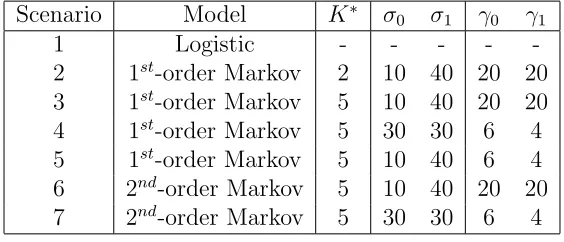
Table 2.1: Seven scenarios in the simulation study.

Scenario Model K∗ σ0 σ1 γ0 γ1

1 Logistic - - - -

-2 1st_{-order Markov} ₂ ₁₀ ₄₀ ₂₀ ₂₀ 3 1st_{-order Markov} ₅ ₁₀ ₄₀ ₂₀ ₂₀ 4 1st-order Markov 5 30 30 6 4 5 1st_{-order Markov} ₅ ₁₀ ₄₀ ₆ ₄ 6 2nd_{-order Markov} ₅ ₁₀ ₄₀ ₂₀ ₂₀ 7 2nd-order Markov 5 30 30 6 4

vectors arewi = (_K1∗, ...,_K1∗), and both benign and malicious programs have the same true number of clusters. Examination of the sensitivity of the model assumption is also given by comparing with the programs generated from the second-order Markovian. Scenarios 6 and 7 are generated from the second-order Markov model, which assumes the current instruction being called in time t not only depends on the instruction at time t−1 but also on the instruction att−2. The transition probability for programs now is a three-dimensional array, where Pslrc = P(Yst = c | Yst−1 = r, Yst−2 = l). The data sets are

again generated from (2.13) similar to the first-ordered Markovian data sets but Zs, Ps, andλi (i= 0,1) are now three-dimensional arrays, and the matrix distributions MD and

MMP are now array distributions, i.e., the vectors across the last dimension of the array for any given values of the first two dimensions are assumed to be Dirichlet. Table 3.2 gives the summary of these seven scenarios.

2.4.2

Simulation results

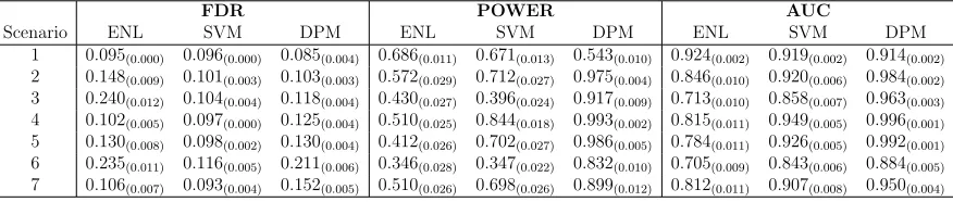
The classification results of the simulation study are presented in Table 2.2. The results show that when the data sets are generated from the logistic regression model, the ENL model performs better than the DPM model by 1% and also better than the SVM by 0.5% in AUC criterion. The ENL model also has higher power than other two methods. Therefore, the ENL model generally performed better than other two methods which is not surprising since the data was originally generated from the logistic regression. On the other hand, when the data sets are generated from the first-order or second-order Markov models, the DPM model outperforms the ENL and the SVM methods signifi-cantly in terms of both power and AUC criterions.

(26)

Table 2.2: FDR, Power, and AUC subscripted with standard errors for the ENL, SVM and DPM models under seven scenarios. The Wilcoxon signed-rank test for the pairwise differences of the ENL, SVM and DPM models under Power, and AUC are all significant.

FDR POWER AUC

Scenario ENL SVM DPM ENL SVM DPM ENL SVM DPM

1 0.095(0.000) 0.096(0.000) 0.085(0.004) 0.686(0.011) 0.671(0.013) 0.543(0.010) 0.924(0.002) 0.919(0.002) 0.914(0.002)

2 0.148(0.009) 0.101(0.003) 0.103(0.003) 0.572(0.029) 0.712(0.027) 0.975(0.004) 0.846(0.010) 0.920(0.006) 0.984(0.002)

3 0.240(0.012) 0.104(0.004) 0.118(0.004) 0.430(0.027) 0.396(0.024) 0.917(0.009) 0.713(0.010) 0.858(0.007) 0.963(0.003)

4 0.102(0.005) 0.097(0.000) 0.125(0.004) 0.510(0.025) 0.844(0.018) 0.993(0.002) 0.815(0.011) 0.949(0.005) 0.996(0.001)

5 0.130(0.008) 0.098(0.002) 0.130(0.004) 0.412(0.026) 0.702(0.027) 0.986(0.005) 0.784(0.011) 0.926(0.005) 0.992(0.001)

6 0.235(0.011) 0.116(0.005) 0.211(0.006) 0.346(0.028) 0.347(0.022) 0.832(0.010) 0.705(0.009) 0.843(0.006) 0.884(0.005)

7 0.106(0.007) 0.093(0.004) 0.152(0.005) 0.510(0.026) 0.698(0.026) 0.899(0.012) 0.812(0.011) 0.907(0.008) 0.950(0.004)

found that when the true number of clustersK∗ increases from 2 to 5 (Scenario 2 and 3), the DPM model has much higher AUC than the other methods. Also, when the between cluster variation increases or within cluster variation decreases (Scenario 3, 4, and 5), the DPM model again has higher power and higher AUC than the other methods. Scenario 4 has the best classification results among all seven scenarios as this setting has the largest between-cluster variation and smallest within-cluster variation. For the last two scenarios where the data are generated from the second-order Markov model, the DPM model out-performs the ENL and SVM by 15% and 5%, respectively, in terms of AUC. In scenario 6 and 7, where the data sets are not generated from first-order Markov model, the FDR of the DPM model is difficult to control around the nominal rate. As the proposed model is constructed under the first-order Markov assumption, this suggests the FDR for our first-order model may be slightly sensitive to model misspecification.

(27)

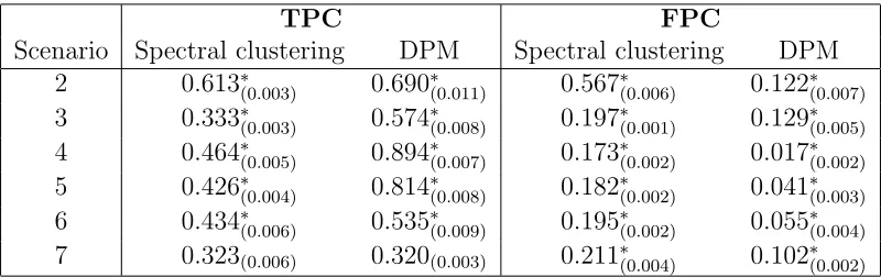
Table 2.3: Overall TPC and FPC subscripted with standard errors for scenario 2-7. (∗ represents the Wilcoxon signed-rank test for the pairwise differences of spectral clustering method and DPM models are shown to be significant, p-value < 0.05. No ∗ represents non-significant.)

TPC FPC

Scenario Spectral clustering DPM Spectral clustering DPM 2 0.613∗₍₀_.₀₀₃₎ 0.690∗₍₀_.₀₁₁₎ 0.567∗₍₀_.₀₀₆₎ 0.122∗₍₀_.₀₀₇₎ 3 0.333∗₍₀_.₀₀₃₎ 0.574∗₍₀_.₀₀₈₎ 0.197∗₍₀_.₀₀₁₎ 0.129∗₍₀_.₀₀₅₎ 4 0.464∗₍₀_.₀₀₅₎ 0.894∗₍₀_.₀₀₇₎ 0.173∗₍₀_.₀₀₂₎ 0.017∗₍₀_.₀₀₂₎ 5 0.426∗₍₀_.₀₀₄₎ 0.814∗₍₀_.₀₀₈₎ 0.182∗₍₀_.₀₀₂₎ 0.041∗₍₀_.₀₀₃₎ 6 0.434∗₍₀_.₀₀₆₎ 0.535∗₍₀_.₀₀₉₎ 0.195∗₍₀_.₀₀₂₎ 0.055∗₍₀_.₀₀₄₎ 7 0.323(0.006) 0.320(0.003) 0.211∗₍₀_.₀₀₄₎ 0.102∗₍₀_.₀₀₂₎

2.5

Analysis of real malicious and benign programs

2.5.1

Data description

Here a modified version of the Ether Malware Analysis framework (Dinaburg et al., 2008) was used to perform the dynamic trace data collection. Collecting dynamic traces can be slow, however, the current implementation is sufficient for a sandbox environment (i.e., the program is passed along to the user that requested it, while being run on a sepa-rate machine devoted to analysis) (Goldberg et al., 1996). For example, many institutions implement an email/http inspection system to filter for spam and malware. Inserting the proposed methodology into this process allows for a more robust approach to analyzing new threats as they are received. The data set used here contains dynamic traces from a five minute run of the program for 1613 malicious and 634 benign programs, respec-tively, for a total of 2247 observations with the number of instruction classes M = 8. This data set is a randomly selected subset of that used in Storlie et al. (2013). There, the malware sample was obtained via a random sample of programs from the website

http://www.offensivecomputing.net/, which is a repository that collects malware

in-stances in conjunction with several institutions.

(28)

Ad-mittedly, this is not a truly random sample from the population of all malicious programs that a given network may see, but it is one of the largest publicly available malware col-lections on the Internet (Quist, 2012). To obtain a sample of benign programs, Storlie et al. (2013) gathered a collection of many programs that were running on Los Alamos National Laboratory (LANL) systems during 2012. If these programs passed through a suite of 25 AV engines as ”clean” then they were treated as benign.

2.5.2

Classification results

The analysis implements a repeated random sub-sampling validation (RRSV) (which is also known as Monte Carlo cross-validation (Picard and Cook, 1984; Xu and Liang, 2001)) to evaluate the classification for the ENL, the SVM, and the DPM models. A 20-fold RRSV method is used for evaluating the classification performance. Each of the RRSV data set is obtained by randomly and equally split the whole samples into training and testing sets. The evaluation will be based on the performances over these 20 RRSV data sets. The FDR, power, and AUC for each model are presented in Table 2.4. The results for the DPM model are presented with truncation values {(K0, K1) = (150,200)}

in (2.13). Other values of (K0, K1) are also implemented but found that a smaller number

of clusters will hurt the classification performances, and a larger number of clusters give similar results. Also, by checking the posterior median of the last mixture probability

wiK (i= 0,1), the values are close to 0.03.

By comparing the DPM and the ENL methods, the DPM has 4.4% higher power than the ENL model and 3.3% higher in AUC. The differences are all statistically sig-nificant. The DPM model performs slightly better than the SVM method under the auc criterion, but the differences are not significant, which indicates that these two methods are competitive. However, the advantage of using the DPM model is that the classifica-tion probability is calculated and can be obtained for each sample. More importantly, a clustering algorithm is the by-product of the DPM model.

2.5.3

Detection under different lengths of traces

(29)

Table 2.4: FDR, Power, and AUC subscripted with standard errors for the ENL, SVM, and the DPM models with {(K0, K1) = (150,200)}.

Method FDR POWER AUC

ENL 0.100(0.000) 0.925(0.004) 0.913(0.002)

SVM 0.100(0.000) 0.982(0.001) 0.943(0.003)

DPM {(150,200)} 0.086(0.002) 0.969(0.002) 0.946(0.002)

RRSV data set. The transition probability matrixPs for each sample is estimated by the corresponding transition matrixZs. Then from this estimates ˆPs, new transition matrices Z_s0 are generated with different lengths of traces. For each sample, we generate lengths of traces from 100 to 35,000. 50 samples are generated under different lengths. Two soft classifiers: the ENL model and the DPM model are compared. Figure 2.1 shows a 95% confidence interval of P(ξs∗ = 1 |Z_s∗,Z) for the ENL model and a 95% credible interval of P(ξs∗ = 1 | Z_s∗,Z) for the DPM model. In sample A, both methods correctly classify the sample from shorter lengths (i.e. two lines are overlapped). In sample B, C, and D, both models correctly classify the sample eventually, however the DPM model requires shorter lengths than the ENL model to achieve narrower 95% interval. In general, the DPM model requires shorter traces to achieve higher probability for accurately classifying a program and gives a narrower 95% intervals than the ENL model. Also, as the length of the trace increases, the probabilities of being malicious go to one for the DPM model for these four examples, which is showing that the flexible DPM model can make better use of the trace data in some cases.

2.5.4

Clustering results

To illustrate how clustering can be used in practice, we first look at the overall cluster-ing between traincluster-ing and testcluster-ing malware for one RRSV data set. Figure 2.2 is the heat map of the training malware along with the testing malware after ordering by their clus-tering probabilities calculated from the DPM model with (K0, K1) = (150,200). Darker

(30)

some similarities between different clusters.

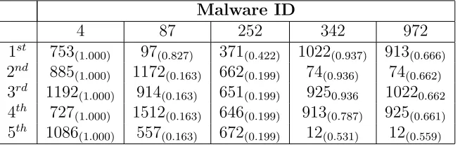
We also choose five malicious testing samples, and present the top five training sam-ples that might be clustered with these testing sets under. From the results in Table 2.5, one advantage of the DPM algorithm is that we could rank the clustering programs and also obtain the pairwise clustering probability instead of the hard clustering method as spectral clustering.

To test the performance of our clustering algorithm in a case where the true clustering is known, we use the case study of the Bagle virus (bag, Accessed 9 December 2013) with the original real data set. The Bagle virus is known to spread via its own smtp engine and by using filesharing networks such as KaZaA. The main purpose of the bagle virus was to create a large botnet for the purpose of spam dissemination. Four programs in the Bagle family are examined: Bagle.n, Bagle.o, Bagle.q and Bagle.r. For each sample, say Bagle.n, the model is trained with the other three programs: Bagle.o, Bagle.q and Bagle.r added to the training programs. We then compute the clustering probability that Bagle.n is clustered with one of Bagle.o, Bagle.q and Bagle.r. The DPM method was able to successful cluster programs Bagle.o, Bagle.q and Bagle.r with at least one member of this family with probability one. However, Bagle.n was only clustered with another member of the family with probability 0.02. Compared to the other variants, Bagle.n is unique as it contains polymorphic code to infect other executables found on a windows system. Our results were able to clearly find this difference. For comparison, we applied the spectral clustering method of Anderson et al. (2012), and found that none of these four programs were clustered with their family, further highlighting the utility of the proposed method.

2.6

Conclusion

(31)

Table 2.5: Clustering results for 5 testing malicious programs (ID:4, 87, 252, 342, 972), each lists the top 5 training samples ID with highest pairwise clustering probabilities in the parenthesis.

Malware ID

4 87 252 342 972

1st ₇₅₃

(1.000) 97(0.827) 371(0.422) 1022(0.937) 913(0.666)

2nd ₈₈₅

(1.000) 1172(0.163) 662(0.199) 74(0.936) 74(0.662)

3rd 1192(1.000) 914(0.163) 651(0.199) 9250.936 10220.662

4th ₇₂₇

(1.000) 1512(0.163) 646(0.199) 913(0.787) 925(0.661)

5th ₁₀₈₆

(1.000) 557(0.163) 672(0.199) 12(0.531) 12(0.559)

(32)

0 5000 15000 25000 35000

0.0

0.2

0.4

0.6

0.8

1.0

Sample A

length of trace

Probability

0 5000 15000 25000 35000

0.0

0.2

0.4

0.6

0.8

1.0

Sample B

length of trace

Probability

0 5000 15000 25000 35000

0.0

0.2

0.4

0.6

0.8

1.0

Sample C

length of trace

Probability

0 5000 15000 25000 35000

0.0

0.2

0.4

0.6

0.8

1.0

Sample D

length of trace

Probability

(33)

(34)

Chapter 3

A nonparametric Bayesian test of

independence

3.1

Introduction

A fundamental statistical task is to determine whether two groups of variables are dependent. For example, in genomic analysis, we might want to test whether two groups of genes are associated to identify dependence between genetic pathways. In the brain imaging research, we may want to discover whether sets of voxels from different parts of the brain are related to explore functional connectivity. In general, high-dimensional data analysis can be simplified by identifying sets of independent variables.

Testing of dependence is often reduced to testing for linear dependence. Pearson cor-relation coefficient is a classical and widely used method for quantifying the strength of linear dependence between two univariate variables. Spearman’s rank correlation coeffi-cient (Spearman, 1904) is a ranked-based version of Pearson correlation coefficoeffi-cient which quantifies monotone correlation. Tests based on correlation are powerful for testing spe-cific types of association, but lose power for other general types.

For testing more general associations, the χ2 _{test of independence and Hoeffding’s}

(35)

contingency table formed by the data, and Wilding and Mudholkar (2008) propose an approximation by using the two Weibull extensions. A relation between the Hoeffding’s test and the χ2 _{test statistics was noted by Thas and Ottoy (2004), and they also}

sug-gested extending the idea of Blum et al. (1961) to a k×k contingency tables, for k >2. More recent methods related to the Hoeffding’s test have been proposed by Heller et al. (2013) and Kaufman et al. (2013). Both of these tests are proved to be consistent under general types of associations. Other methods for testing for independence include the distance correlation test of Szekely et al. (2007) and the maximal information coefficient of Reshef et al. (2011). Both the tests of Heller et al. (2013) and Szekely et al. (2007) can be extended to higher dimensions for testing joint independence of two or more random vectors. Several Bayesian methods are introduced for testing of independence. The sim-plest test of linear dependence between two univariate random variables can be achieved by fitting a linear model and inspecting the posterior distribution of the correlation coef-ficient. Other methods were proposed for testing of independence based on a contingency table (Nandram and Choi, 2006, 2007; Nandram et al., 2013).

In this chapter, we propose a nonparametric Bayesian test of independence between two groups of variables. We test the null hypothesis of independence and the alternative hypothesis of dependence. We specify nonparametric Bayesian models for the response density under both hypotheses. Under the null hypothesis, the joint distribution is taken to be the product of two independent densities, both with nonparametric priors; under the alternative, the full joint density has a nonparametric prior. The test is based on the posterior probability of the alternative hypothesis. By specifying nonparametric Bayesian models under each hypothesis, we obtain an extremely flexible test which can capture both linear and complex nonlinear relationships between groups of variables.

(36)

3.2

Statistical model

LetX1 ∈RD1 andX2 ∈RD2 be random vectors inD1 andD2dimensions, respectively,

and denoteX = (X1,X2). The objective is to test whetherX1 andX2 are independent.

The hypotheses are

H0 : X1 and X2 are independent and f(X) =f1(X1)f2(X2)

H1 : X1 and X2 are dependent and f(X) cannot be factorized

In other words, when they are independent, the joint density can be factorized as the product of two lower-dimensional densities.

Under both hypotheses, the densities are modeled using Dirichlet process mixture (DPM) priors as introduced in Chapter 2. Under H0,f1(X1) andf2(X2) follow

indepen-dent DPM priors; under H1 when X1 andX2 are not independent, the joint distribution

is assumed to follow a DPM prior. The following subchapters describe the independent and joint DPM priors.

3.2.1

The independent DPM prior

When X1 and X2 are independent, fj(Xj), j = 1,2, are assumed to follow the DPM prior independently. The DPM prior can be written as the infinite mixture

fj(Xj) =

∞

X

l=1

wljφj(Xj | µlj,Σj), (3.1)

where wlj is the mixture weight, φj is assigned to be the Dj−dimensional multivariate normal distribution (MVN) in this analysis, µ_lj is the mean vector of the lth _mixture component, and Σj is the covariance matrix.

The mixture weightswlj are modeled by the stick-breaking construction with concen-tration parameter dj. The weights wlj are modeled in terms of latent vlj ∼ Beta(1, dj). The first weight is w1j =v1j. The remaining elements are modeled as wlj =vlj

Ql−1 i=1(1−

vij), where Ql−1

i=1(1−vij) = 1− Pl−1

i=1wij is the remaining probability after accounting first

l−1 mixture weights. The number of mixture components is truncated by a sufficiently large number K (i.e. l = 1, ..., K), where the last term vK is fixed to be 1 to ensure that PK

(37)

The mean vectors µ_lj have priors µ_lj ∼ MVN(0,Ωj). The covariance matrices Σj and Ωj are parameterized as Σj = rSj, and Ωj = (1−r)Sj. Under this model, Sj is the covariance matrix for Xj marginally over the mixture means µlj, and r is the pro-portion of the total variance attributed to the variance within each mixture component. The marginal covariance Sj is assigned to have inverse Wishart prior distribution, and to facilitate computing, the prior of r is a discrete uniform distribution with support

r∈ {0,0.01, ...,1}. The concentration parameter dj has prior distribution Gamma(a, b).

3.2.2

The joint DPM prior

When X1 and X2 are not independent, f(X) is assumed to follow the joint DPM

prior

f(X) =

∞

X

l=1

wlφ(X | µl,Σ), (3.2)

where wl is the mixture weight, φ is the (D1+D2)−dimensional MVN distribution, µl is the mean vector of the lth mixture component, and Σ is the covariance matrix. The number of mixtures is truncated by the same numberK as in the independent model. The mixture weightswl are again modeled by the stick-breaking algorithm with concentration parameter d. The mean vectors µ_l have priorsµ_l ∼φ(0,Ω). The covariance matrices Σ

and Ω are modeled as Σ = r·diag(S) and Ω = (1−r)S, where S is the covariance matrix for X, and diag(S) is the diagonal form of S. In other words, under the joint DPM prior, we assign non-diagonal structure for the Ω, and diagonal structure for the

Σ. The priors forS, r, andd are the same as in the independent DPM prior.

3.2.3

Bayesian test of independence

The Bayesian hypothesis test of independence is based on the Bayes factor (BF)

BF = P(H1 | X)/P(H0 | X)

P(H1)/P(H0)

= P(X | H1)

P(X | H0)

. (3.3)

The null is rejected if BF> T, whereT is a threshold parameter. The threshold parameter

T can be chosen based on rules of thumb about the weight of evidence favoring H1. For

example, Kass and Raftery (1995) suggest that BF = 10 is a strong evidence for H1.

(38)

error rate. In the analysis of genetic data in Chapter 3.5, multiple tests are performing simultaneously, therefore we select T to control the Bayesian false discovery rate.

3.3

Computing details

Computing the Bayes factor requires computing the posterior probability of each hypothesis. This is accomplished using a reversible jump MCMC (RJMCMC) algorithm as described below.

3.3.1

Reparameterization and hyperparameters

The updating algorithm of the DPM prior is facilitated by introducing the clustering model as in Chapter 2. The mixture form in (3.1) can be written as

fj(Xj |gj =l) =φj(Xj |µlj,Σj),

which draws an auxiliary cluster label gj ∈ {1, ..., K} with P(gj = l) = wlj. Similarly, the model in (3.2) is equivalent to

f(X |g =l) =φ(X |µ_l,Σ),

with cluster labelg and P(g =l) = wl. Under the clustering model, the full conditionals of all the parameters are conjugate.

In addition, we introduce model indicator parameter M, where

M ∈

(

I if X1 and X2 are independent (H0 is true)

J if X1 and X2 are not independent (H1 is true).

Under each MCMC step, we propose a new indicatorM0 in the Markov chain, and decide whether to accept the new status M0. The probability P(H1 | X) is then approximated

by PN

i=1I(M(i) = J)/N, where N is the number of MCMC samples and M(i) is the

model status for the ith _{MCMC sample.}

Throughout this chapter, we let the number of mixture components truncated at

(39)

Table 3.1: Hyperparameters (a, b) under different sample sizes n.

n a b

100 1.5 2.5 200 1.0 4.0 300 1.0 4.5 500 0.8 4.6

3.3.2

Pseudo code for the DPM test of independence algorithm

Let ΘM denote the DPM parameters (ΘM = {µ11, ...,µK2, r, S1, S2, w11, ..., wK2,

d1, d2} if M = I, and ΘM ={µ1, ...,µK, r, S, w1, ..., wK, d} if M =J). The algorithm of the DPM test of independence is described as follows:

Step 0: Select initial values for M and ΘM.

Step 1: Update ΘM given M using the Gibbs sampling.

Step 2: Update M given the parameters ΘM.

Step 2.1: Generate proposed model status M0 with P(M0 =I) = P(M0 =J) = 0.5.

Step 2.2: If M =M0, then so back to Step 1.

Step 2.3: If M = I and M0 = J, then propose Θ_M0 required for the joint DPM prior (H1).

Step 2.4: IfM =J and M0 =I, then propose Θ_M0 required for the independent DPM prior (H0).

Step 2.5: Accept M0 with probability min{1, α(M, M0)}.

Step 3: Back to Step 1.

The full conditionals requires for Step 1 are all standard and are given in Appendix B.1.1 forM =I, and Appendix B.1.2 for M =J. Details on the RJMCMC steps are provided below in Chapter 3.3.3.

3.3.3

Steps of the RJMCMC algorithm

(40)

updates.

Under the current model statusM, the propose model statusM0 is randomly assigned to be either I or J with acceptance probability min{1, α(M, M0)}, where

α(M, M0) = lM 0 ·π

M0 ·qM |M0 ·pM0→M

lM ·πM ·qM0 |M ·pM→M0

|J|, (3.4)

where lM and πM are the likelihood function and the prior distribution under modelM,

q_M0

|M is the candidate distribution of the parameters when proposing for modelM 0

un-der modelM,p_M_→_M0 is the probability of proposingM

0

conditional on the current status

M, and|J|is the Jacobian. AsM0 is randomly picked from{I, J},p_M_→_M0 andp

M0→M are equal in the algorithm. Note that whenM =M0, it becomes the usual fixed-dimensional MCMC algorithm as α(M, M0) = 1; when M 6= M0, the candidate distribution of the parameters q is then for balancing the parameter spaces between the independent and joint models.

Recall that ΘM and ΘM0 denote the DPM parameters under modelsM and M 0

, re-spectively, and the truncated numberK under both models are assigned to be identical. We first examine the case whenX1andX2are univariate random variables (D1 =D2 = 1)

with the current model status M = I, and the proposed model is M0 = J. Denote the covariance matrix under the joint model as S = S112 S11S22ρJ

S11S22ρJ S222

. We assign the 2×K

mean vector µto be the same in both the independent and joint DPM models. Also, we assign the variances S2

11 and S222 , and r to be the same across different model statuses.

Therefore, this move only requires proposing the parameters under the joint DPM prior in (3.2): the cluster labelg0_J,ρ0_J, the concentration parameterd0_J, and the mixture weights w0_J. The concentration parameter d0_J is proposed by d_J0 ∼Gamma( ¯dI,1), where ¯dI is the mean of dI, and then the mixture probabilities w0J is proposed from the stick-breaking procedure with concentration parameter d0_J. The cluster label g_J0 is proposed from the full conditional distribution given in Appendix B.1. The details of the mapping for each parameter is described in the end of this section.

Conversely, if the current model status is M = J and the proposed model status is

(41)

B.1.

For dimension matching under the RJMCMC algorithm, the bijection map is de-scribed below for the case where M = I and M0 = J. The reverse move uses the same map. Let

θM = {µ, S11, S22, r,wI, dI, gI}

u = {ρ0_J,w0_J, d0_J, g_J0}

θM0 = {µ, S₁₁, S₂₂, r,w_J,d_J, g_J, ρ_J}

u0 = {w0

I, d

0

I, g

0

I}.

Then we assign ΘM ={θM, u}, ΘM0 ={θ_M0, u0}. The bijection function h has the form

h(ΘM) = h(θM, u) = ΘM0 ={θ_M0, u0},

which is a one-to-one bijection map with: wI → w0I, dI → d0I, gI → g0I, ρ

0

J → ρJ, w0_J →wJ, d0J →dJ, and gJ0 →gJ. Hence, the Jacobian|J|=

∂(θ0_M0,u0) ∂(θM,u)

= 1.

WhenD1+D2 >2, the transition of the covariance matrices between the independent

and joint models becomes more complicated as the off-diagonal elements are harder to propose than in the bivariate case. One way to alleviate this concern is to assume the covariance matrix S under the joint model is a block-diagonal matrix S = S1 0

0 S2

, where Si is a Di ×Di covariance matrix of Xi for i = 1,2. However, in the simulation study and the real data analysis of this chapter, we will focus on the case whereX1 and

X2 are univariate random variables.

3.4

Simulation Study

(42)

3.4.1

Data generation

The seven different types of data sets are described as follows. Scenarios 5 and 6 are designed from Kaufman et al. (2013).

1. Independent normal (Null): Xj ∼N(0,1), for j=1,2. 2. Bivariate normal (BVN): (X1, X2)∼BVN

0, 1_ρρ₁

, whereρ= 0.2.

3. Horseshoe (HS): X1 ∼N(0,1), X2 | X1 ∼N(ρX12,1), where ρ= 0.2.

4. Cone: X1 ∼U(0,1), X2 | X1 ∼N [0,(ρX12+ 0.1)2], where ρ= 0.1.

5. W: X1 ∼ 1_n

Pn

i=1U(ai, ai + ₃1), X2 | X1 ∼ U

3(X2

1 − 1 2)

2_,_{3(1 +}_X2 1 −

1 2)

, where

a1 =−1,n is the number of samples, andai =ai−1+ _n2, for i >1.

6. Circle: (X1, X2)∼ 1_nPn_i₌₁BVN

h

θi,

1 9 0

0 ₆₄1

i

, where θi = [sin(aiπ),cos(aiπ)], and ai is defined as in W.

Each scenario is generated with the algorithms introduced above with sample size

n = 100,200, and 500. Then for each dimension, we standardize the data to have mean zero and variance one. We plot the data when n= 200 in Figure 3.1 along with the true density. The responses are dependent for designs 2-6. Design 3-6 are all examples of the challenging dependent but uncorrelated and thus the usual test of correlation will miss this dependence.

3.4.2

Methods for testing of independence

We compare six methods in the simulation study. Each method is controlled to have type I error rate approximately equal to 0.05.

1. Linear regression (LR): The model X2 = β0 +β1X1 +, ∼ N(0,1) is fitted by

least squares and the linear association is determined by the test of β1 = 0.

2. E-statistics (ES) (Szekely et al., 2007): The testing procedure is by calculating the distance covariance between X1 and X2. Details are given in Appendix B.2.

(43)

−3 −2 −1 0 1 2 −2 −1 0 1 2 Null X1 X2

−3 −2 −1 0 1 2

−2 −1 0 1 2 BVN X1 X2

−3 −2 −1 0 1 2

−2 −1 0 1 2 HS X1 X2

−1.5 −0.5 0.5 1.5

−3 −2 −1 0 1 2 3 Cone X1 X2

−1 0 1

−1 0 1 2 W X1 X2

−2 −1 0 1

−1.5 −1.0 −0.5 0.0 0.5 1.0 1.5 Circle X1 X2

Figure 3.1: True log density (background color) and one simulated data set (points) for each simulation design.

4. Data Derived Partitions method (DDP) (Kaufman et al., 2013) with 3×3 contin-gency tables: The DDP method is similar to the HHG method, but only designed for univariate random variables. The test statistic is based on the sum of all likeli-hood ratio tests of 3×3 contingency tables formed by the observed values. More details are given in Appendix B.4.

(44)

6. The DPM test of independence (DPM): The proposed test is described in Chapter 3.2. TheX is first marginally transformed to the normal scores, which transforms the data to the expected values of the order statistics of a same-size standard normal distribution. The normal score transformation is to make the proposed method becomes a distribution-free testing procedure. Therefore, the threshold for the BF in Chapter 3.2 can be determined by the permutations of the transformed data. The threshold T for the Bayes factor is computed from 300 permutations of the sample.

3.4.3

Simulation results

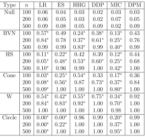
The results are presented in Table 3.2 with sample sizesn= 100, 200 and 500. The first three rows of the table are the type I error rate for each method under different samples sizes, which is controlled for all methods (Type I error rate is between 0.03 to 0.09). The following rows give the power of each method under different scenarios and sample sizes. It is clear that as the sample size n increases, the powers increase for all the methods except the LR method under the HS, Cone, and Circle scenarios because of the nonlinear associations of these scenarios.

When the data are generated from bivariate normal distribution, the LR method has the highest power. This is expected because the LR method is theoretically the most powerful test under this scenario. The ES and DPM tests are the second best among other comparing tests.

The DPM test outperforms all other methods when data are generated from the HS and the W shapes. Under the Cone shape data, the HHG and the DPM tests both perform well. For the Circle design, the HHG, DDP, and DPM tests all have power greater than 0.9 starting from small sample sizes, and the ES and MIC have lower power.

(45)

Table 3.2: Power of each test (columns) for each simulation settings and sample size n

(rows). A ∗ indicates that the power is significantly different than the power of DPM test.

Type n LR ES HHG DDP MIC DPM

Null 100 0.06 0.04 0.03 0.02 0.03 0.03 200 0.06 0.05 0.03 0.02 0.07 0.05 500 0.09 0.08 0.05 0.09 0.02 0.09 BVN 100 0.57∗ 0.49 0.24∗ 0.38∗ 0.13∗ 0.43 200 0.84∗ 0.78 0.37∗ 0.61∗ 0.25∗ 0.76 500 0.99 0.99 0.83∗ 0.99 0.40∗ 0.99 HS 100 0.11∗ 0.22∗ 0.42 0.39 0.12∗ 0.44 200 0.05∗ 0.48∗ 0.53∗ 0.60∗ 0.25∗ 0.68 500 0.10∗ 0.96 0.99 1.00 0.42∗ 1.00 Cone 100 0.03∗ 0.25∗ 0.54∗ 0.33 0.17∗ 0.36 200 0.08∗ 0.56∗ 0.87 0.73∗ 0.37∗ 0.84 500 0.09∗ 1.00 1.00 1.00 0.80∗ 1.00 W 100 0.54∗ 0.42∗ 0.55∗ 0.75∗ 0.34∗ 0.92 200 0.84∗ 0.83∗ 0.92∗ 1.00 0.70∗ 1.00 500 1.00 1.00 1.00 1.00 0.98 1.00 Circle 100 0.00∗ 0.00∗ 0.96 0.99 0.20∗ 0.99 200 0.00∗ 0.22∗ 1.00 1.00 0.37∗ 1.00 500 0.00∗ _1.00 _1.00 _1.00 ₀_.₉₅∗ _1.00

3.5

Real data analysis

We compare the six methods in the simulation study on the gene expression data set from Hughes et al. (2000). Studies of associations between genes can be found in de la Fuente et al. (2004) and Bhardwaj and Lu (2005). The number of observations is

n = 300 for each gene, and we select 94 genes on chromosome 1 after removing samples with missing values. The objective is to test the pairwise associations within these 94 genes. A total of 94

2

(46)

The Cohen’s κ statistic (Cohen, 1960) is used to measure agreement between tests. The κ statistic is

κ= Pa−Pe 1−Pe

,

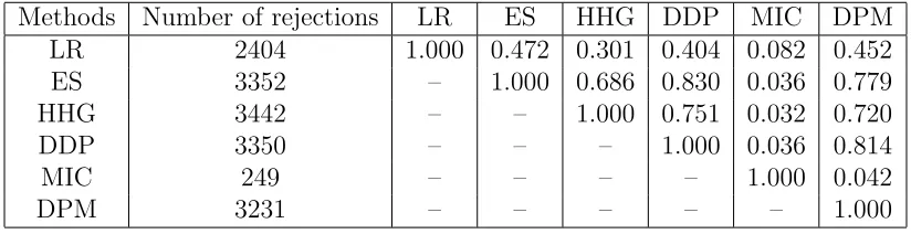
wherePa is the proportion of agreements between the two methods among theN = 4371 tests, and Pe is the theoretical proportion of agreements under independence. Larger values ofκrepresents more agreement between the tests. The number of rejections among

N = 4371 tests and the κ statistics of pairwise methods are presented in Table 3.3.

Table 3.3: Numbers of rejections (of the N = 4371 tests), and Cohen’s κ statistics for each pair of methods.

Methods Number of rejections LR ES HHG DDP MIC DPM

LR 2404 1.000 0.472 0.301 0.404 0.082 0.452

ES 3352 – 1.000 0.686 0.830 0.036 0.779

HHG 3442 – – 1.000 0.751 0.032 0.720

DDP 3350 – – – 1.000 0.036 0.814

MIC 249 – – – – 1.000 0.042

DPM 3231 – – – – – 1.000

The κ statistics show that the ES, HHG, DDP, and the DPM tests have similar testing powers in this gene expression data sets, and the number of rejections among these tests are similar (3231 to 3442). The LR test only captures the linear associations between genes, and the MIC has the lowest power as in the simulation study.

(47)

30 versus gene 6) are the cases where only the LR, ES and DPM tests flag associations between genes. These three tests are powerful in testing the linear associations, and the figure shows linear relationships between genes in these two pairs.

−1.0 −0.6 −0.2

−0.4

0.0

0.4

94 vs 8

Gene8

Gene94

−1.0 −0.5 0.0 0.5

−2.5

−1.5

−0.5

88 vs 15

Gene15

Gene88

−1.0 −0.5 0.0

−0.8

−0.4

0.0

17 vs 1

Gene1

Gene17

−1.5 −1.0 −0.5 0.0 0.5

−2.0

−1.0

0.0

89 vs 24

Gene24

Gene89

−1.5 −1.0 −0.5 0.0

−2.5

−1.5

−0.5

92 vs 2

Gene2

Gene92

−0.2 0.0 0.2 0.4 0.6

−2.0

−1.0

0.0

30 vs 6

Gene6

Gene30

Figure 3.2: Six pairs of genes where there are disagreements among the tests. The red lines are the linear fitted lines.

3.6

Conclusion

(48)

and nonlinear relationships.

(49)

Chapter 4

Efficient multidimensional Bayesian

density estimation using factored

densities

4.1

Introduction

In this chapter, we propose a new method to estimate an unknown probability density function. While there are many classical methods that are efficient in low dimensions, the objective of this chapter is to estimate the density when the dimension is moderate or large. Some