Contributions to Spatial Statistics and Big Data Analytics.

(1)

ABSTRACT

CHAKRABORTY, ARNAB. Contributions to Spatial Statistics and Big Data Analytics. (Under the direction of Soumendra Nath Lahiri).

With the proliferation of sensor-related technologies and advancement of global

po-sitioning system in recent years, large-scale weather data can be captured through the

microsensors installed in mobile devices. As this information is gathered by various

mo-bile applications, e.g. WeatherSignal, AccuWeather, DarkSky etc., often this type of data

is referred as ‘crowdsourced’ weather data, i.e. information collected through users of

var-ious mobile applications. Though these datasets has the potential to be used for weather

analysis, especially in ‘hyper-local’ regions around population centers, due to the

ama-teur quality of the micro-sensors, non-laboratory environement, indoor-outdoor activity

of the users and many such reasons, the quality of the observations is compromised.

Hence, a robust scalable statistical methodology to analyze these varying-quality spatial

data is needed which, along with the variety and velocity of the big-data, incorporates

the veracity of the information as well.

In Chapter 2, a method of veracity scoring has been introduced for geostatistical data.

In addition, a statistical methodology to analyze noisy spatial data has been proposed

which takes the veracity information of the observations into account and thus,

pro-vides robust inference and prediction. The advantage of the proposed method has been

showcased through simulations and several case-studies involving crowdsourced ambient

temperature data over the contiguous USA. Chapter 3 extends the discussion of veracity

score based methods in more theoretical details. Large sample properties of the veracity

score based parameter estimators has been analyzed and their asymptotic efficiency as

(2)

attentions has been shifted to anisotropic covariance modeling which is one of the most

important research area of interest in spatial statistics. A copula-based method has been

proposed that incorporates the directional variogram analysis to construct an admissible

joint covariance over the space. Finally, the large sample properties of the covariance

(3)

(4)

Contributions to Spatial Statistics and Big Data Analytics

by

Arnab Chakraborty

A dissertation submitted to the Graduate Faculty of North Carolina State University

in partial fulfillment of the requirements for the Degree of

Doctor of Philosophy

Statistics

Raleigh, North Carolina

2019

APPROVED BY:

Alyson Wilson Donald Martin

William Boettcher Soumendra Nath Lahiri

(5)

DEDICATION

To Maa, Baba, and Priyanka

(6)

BIOGRAPHY

Arnab Chakraborty was born on September 13, 1992 in Chinsurah, West Bengal,

In-dia. He completed his secondary education (till 10th standard) in 2008 and his higher

secondary education in 2010 from Hooghly Collegiate School, Chinsurah. Having keen

interest in mathematical sciences, Arnab joined Indian Statistical Institute (ISI), Kolkata

among the top 40 students from all over India for his undergraduate study in Statistics

and Mathematics. In 2013, he received B.Stat (Hons.) degree in First Division with

Dis-tinction from ISI, Kolkata. He continued to pursue his master’s degree in Statistics at

ISI, Kolkata and graduated with M.Stat with First Division in 2015. Arnab then joined

the Department of Statistics at North Carolina State University as a graduate student

in 2015. Under the guidance of Dr. Soumendra Nath Lahiri, he successfully earned his

(7)

ACKNOWLEDGEMENTS

It has taken me four years to finish this dissertation and it would not have been possible

without the support and guidance of a bunch of lovely people, whom I really feel fortunate

to have in my life. Though I can never thank them enough for their contributions to my

accomplishments, I want to acknowledge their efforts briefly in this section.

First of all, I want to thank my family members for their constant love and support

throughout my life. I think I owe all my accomplishments to my parents, Mr. Amit

Kumar Chakraborty and Mrs. Lakshmi Chakraborty. Their efforts since my childhood

have helped me stay focused towards achieving my goals. Next, I want to mention my

lovely girlfriend and my partner in life, Priyanka. Every time I have fallen down, either

mentally or physically, even being nearly 9000 miles away from me, she has always been

there for me. She has encouraged me through every hurdle of my life in the last three

years and has always believed in me, when at times, even I did not believe in myself.

The person I want to thank the most for this dissertation is my advisor Dr. Soumendra

Nath Lahiri. I am indebted to him for his care, guidance and encouragement as well as

his patience with me. Often I was stuck with doubts about my research and he always

clarified those in a way that was best for me to comprehend. His approach of tackling any

mathematical or statistical research problem is something that I have always tried to learn

and will continue to follow in my future. Apart from his guidance in my research, I am

grateful for his teachings in two of the advanced courses that I took in the first two years of

my graduate curriculum. It was his way of teaching a very complicated topic fairly simply

that made me interested to work in spatial statistics under his supervision. I also want

to thank Dr. Alyson Wilson, Dr. Donald Martin and Dr. William Boettcher for agreeing

(8)

helped improve this dissertation significantly. Apart from my advisory committee, I want

to thank Dr. Eric Laber, Dr. Eric Chi, Dr. Jason Osborne, Dr. Leonard Stefanksi and

Dr. Marie Davidian for teaching me important concepts and topics in Statistics during

the course of my stay at NC State. I also want to thank our staff at the Department

of Statistics, especially Lanakila and Alison, for helping me out with official issues, as

well as Terry and Chris for being patient with my computational issues that I have faced

during my doctoral degree program.

Before coming to NC State, back in India, I was fortunate to have great teachers and

I am indebted to each and every one of them. I want to particularly thank Nimai Kundu,

Amitabha Pal and Tapan Kumar, whose teachings in my high school days helped me grow

an interest to pursue Mathematics and Statistics in my higher studies. I am and forever

will be immensely grateful to Padma Shri Prof. Jayanta K. Ghosh for his care, guidance

and encouragement during my summer internship at Department of Statistics in Purdue

University. I also want to thank Dr. Sourabh Bhattacharya, Dr. Arijit Chakraborty and

Dr. Ayan Basu for their teachings that have helped me get a rigorous training in Statistics

during my bachelor’s and master’s degree program.

In these four years of my life I have come across a bunch of people who has made my

stay at Raleigh smooth and enjoyable. First, I want to thank Dr. Indranil Sahoo (Sahoo

Da), Dr. Arnab Hazra (Hazra Da), Salil Koner and Dhrubajyoti Ghosh (DjG) – who are

probably the best roommates to live with. I think the things that I have enjoyed the

most during these four years are things like watching movies or TV series with them,

long discussions or debates with them on all types of topics, arranging our regional

festivals and departmental events together etc. Their companionship and encouragement

have made me get through many tight situations over the years and never made me feel

(9)

(Ghoshal), Rahul Chak, Pulama Di, Moumita Di, Debraj Da, Priyam Da (Ala Da),

Souvik Da for making my life more enjoyable in Raleigh. Special thanks goes to Jim,

Michele, Yun Hee and John for welcoming me to their life, which made me realize I got a

home, so far away from home. Not to forget some of my friends from undergraduate and

graduate years in ISI, Kolkata: Atanu, Indranil (U), Diganta, Arnab (Chow), Debojyoti

Da, Sourav (Chhutku), Sandipan (Mamba), Indrayudh who made the transition of my

life from childhood to adulthood smooth and enjoyable.

Finally, I want to thank the Department of Statistics at NC State for giving me the

opportunity to pursue a doctoral degree in the topic of my interest and their constant

(10)

LIST OF TABLES

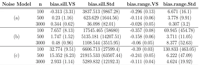
Table 2.1 Performance of the VS-based methodology and standard approach in

estimating covariance parameters on varying-quality observations. . . . 32

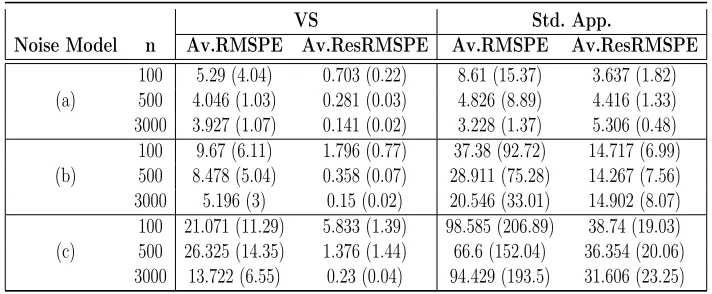
Table 2.2 Prediction performance of the VS-based methodology and standard

ap-proach on varying-quality observations without any reference data. . . . 34

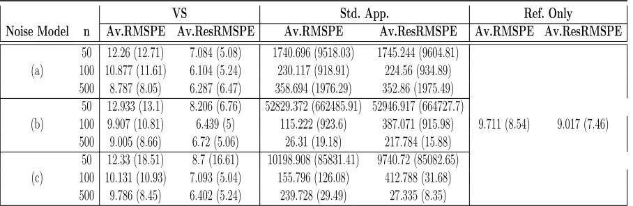
Table 2.3 Performance of hyper-local predictions using the VS-based methodology,

the standard approach and global predictions using reference data only. For these simulations we used reference data with sample sizem= 100. 35

Table 2.4 Estimated Mat´ern parameters. . . 38

Table 2.5 Predictions using both the VS-based and standard approach at the

ground-stations with crowdsourced observations in proximity. . . 46

Table 3.1 Empirical mean squared errors (MSE) of the VS-based and least squares

(LS) based regression parameter estimator; relative efficiency (R.E.) of the Median-VS estimator with respect to that of OLS estimator – for varying noise model parameters (σA, σM, qe) and varying sample sizes

(n). For each sub-table, the other noise parameters are fixed at their first value, e.g. for the sub-table (top) with varyingσA, the other parameters

are fixed atσm= 0.447 and qe = 0.95. . . 73

Table 3.2 Empirical mean squared errors (MSE) of the VS-based and weighted

least squares (WLS) based covariance parameter (psill : σ2, range : ρ) estimator for varying noise model parameters (σA, σM, qe) and varying

sample sizes (n). For each sub-table, the other noise parameters are fixed at their first value, e.g. for the sub-table (top) with varyingσA, the other

parameters are fixed atσm= 0.447 and qe= 0.95. . . 75

Table 3.3 Estimated Mat´ern parameters. . . 78

Table 3.4 Time comparison between VS-based and robust-REML. Machine

con-figuration: DELL R7425 Dual Processor AMD Epyc 32 core 2.2 GHz machines with 512GB RAM each running 64Bit Ubuntu Linux Version 18.04. . . 80

Table 4.1 Empirical mean squared errors (MSE) of the WLS-based covariance

pa-rameters estimators for the Exponential-Gaussian Bivariate Normal Copula-based model. The true values of the parameters are: αe = 2, αg = 4,

ρ= 0.5 andσ2 = 3. . . 126

Table 4.2 Performance under correct model: Spherical-Gaussian-Normal-Copula. . 127

(13)

(14)

LIST OF FIGURES

Figure 2.1 Spatial plots of the crowdsourced and NOAA ground-station data.

(c) - (f) show zoomed hyper-local versions of the crowdsourced

WeatherSignal (c - d) and NOAA station data (e - f). . . 9

Figure 2.2 Empirical distribution of the crowdsourced average temperatures

in the regions from Figure 2.1 for Brooklyn, NY (left) and Detroit, MI (right). Blue vertical lines represent the average ground-station

values in the considered regions. . . 10

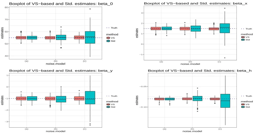
Figure 2.3 Performance of the VS-based and standard regression parameter

estimators for analyzing varying-quality observations (sample size

n= 500) without reference data. . . 31

Figure 2.4 Example sampling points for the simulations. . . 33

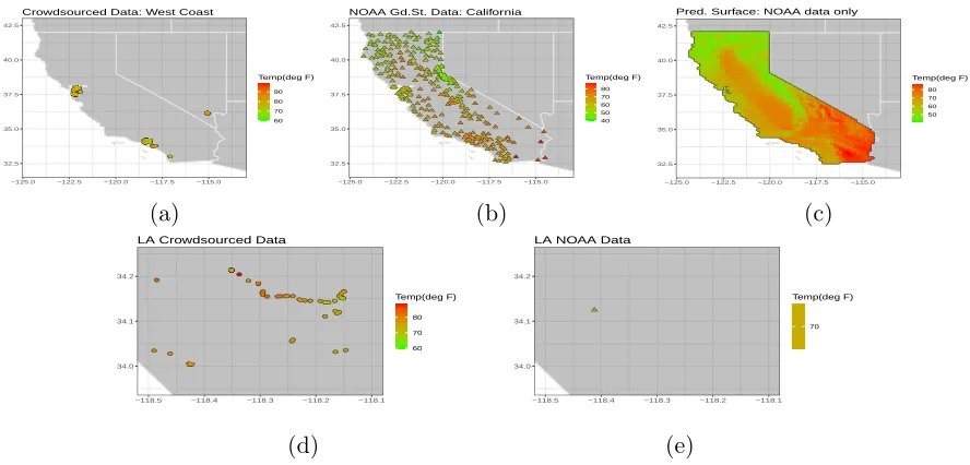
Figure 2.5 (a) Crowdsourced observations in CA; (b) Available ground-station

ob-servations; (c) Prediction surface using the standard approach on the ground-station data; (d) Crowdsourced observations in a hyper-local region around Los Angeles; (e) ground-station observations in a hyper-local region around Los Angeles. . . 37

Figure 2.6 Variogram estimation. . . 38

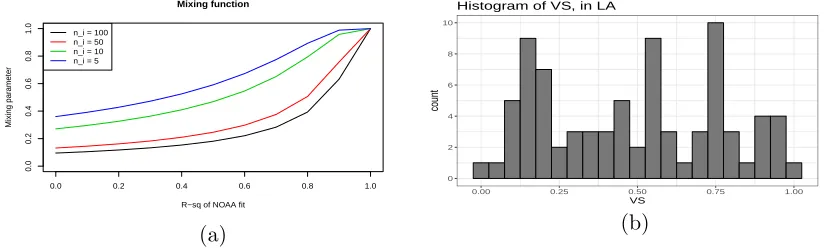
Figure 2.7 Mixing function (a) and the histogram of the veracity scores (b) for the

crowdsourced observations in Los Angeles. . . 39

Figure 2.8 Histograms of the observed residuals (a) and VS-based smoothed

resid-uals (b) and the VS-based variogram fitting (c) for optimal q= 0.8. . . 40

Figure 2.9 (a) Hyper-local version of the same surface as in Figure 2.5c; (b)

Predic-tion surface obtained by the VS-based technique on the crowdsourced data in Los Angeles; (c) Residual kriging variance for the predictions using NOAA data only (d) Residual kriging variance for the predictions using the VS-based predictions with crowdsourced data; (e) the % in-crease in the margin of error for the VS-based predictions as compared to the predictions with NOAA data . . . 41

Figure 2.10 (a) Ground-station observations in the selected hyper-local region; (b)

Crowdsourced observations in the same region (c) Prediction surface ob-tained by standard analysis of NOAA ground-station data; (d) Predic-tion surface obtained by the VS-based technique on the crowdsourced data; (e) Residual kriging variance for predictions using NOAA data only; (f) Residual kriging variances for the predictions using the crowd-sourced data; (g) Percent increase in the margin of error for the VS-based predictions compared to the predictions with NOAA data. . . . 44

Figure 2.11 The increase in margin of error for the standard approach in hyper-local

(15)

Figure 3.1 Spatial plots of the coalash data (a) and VS of the observations (b). 76

Figure 3.2 VS-based smoothing of residuals: histogram of observed residuals

from VS-based regression (a), histogram of smoothed residuals (b),

qqplot of observed residuals (c), qqplot of smoothed residuals (d). 78

Figure 3.3 Variogram estimation. . . 78

Figure 3.4 Prediction comparison between VS and robust-REML: histogram of

prediction errors of VS-based (a) and robust-REML (b) approach; empirical c.d.f. of prediction errors (c) and relative efficiency in

terms of margin of prediction errors of VS w.r.t. robust-REML (d). 79

Figure 4.1 Illustration of the covariance functions obtained by combining univariate

Exponential and Gaussian covariances. . . 118

Figure 4.2 Illustration of the covariance functions obtained by combining two

uni-variate Mat´ern covariances.. . . 120

Spherical and Gaussian covariances. . . 121

Exponential and Gaussian covariances using FGM copula.. . . 122

Figure 5.1 In this figure we plotted the hourly averages of the real-time temperature

readings for two selected locations and showed how spline regression is fitted to estimate the hourly pattern for that particular day. The x-axis is shifted−5 hours to make the plot look reasonable as the temperature pattern is cyclical over the hours. . . 138

Figure 5.2 Possible choices of theφ-function in the definition of VS. . . 139

Figure 5.3 VS-based smoothing of the observed residuals.q= 1.5 for the smoothed

(16)

Chapter 1 Introduction

Spatial statistics is a field of science that is concerned with the theory and applications

re-lated to spatially indexed physical processes such as ambient temperature, precipitation,

humidity, air pollution, soil acidity, soil quality etc. Introduced as a statistical

method-ology to predict ore reserve in mining engineering in early 1960s, in the last 50 years

spatial statistics has emerged as a hybrid discipline of statistics, mathematics, geology

and computer science with lots of applications in forestry, agriculture, climatology,

me-teorology, weather analysis, epidemiology, economics, image processing and many other

related fields. In the last two decades, a handful number of works have been added to

the literature of spatial statistics, and a significant number of these researches are

per-tained to meteorology with a major focus on weather analysis. Weather analysis involves

structure exploration of the key atmospheric features – for example temperature, wind

velocity, air pressure etc. – and prediction of the key weather elements based on the

information collected at the meteorological stations or through satellite images. Though

prediction of weather conditions in future based on the information in past – which is

(17)

weather-related processes has similar importance as temporal prediction because, as

men-tioned by Cressie (1993), “spatial prediction is just as important as temporal prediction,

because people living those cities and rural districts without monitoring stations have the

same right to know how little or how much their water or their air is polluted.” Most of

the spatial prediction of weather-related processes are based on data collected by

high-performance sensors at meteorological stations or images captured by high-resolution

cameras in satellites. Recently, with the advancement of mobile sensor-related technology,

geo-tagged weather information is being collected by micro-sensors installed in mobile

devices and gathered by mobile weather applications like AccuWeather, WeatherSignal

etc. These datasets are often referred as ‘crowdsourced’ weather data as the information

is coming from the mobile application users. Standard methodologies in geostatistics

or spatial statistics is not directly applicable to these mobile sensor-generated data as

quality of the observations are often hampered in crowdsourced datatsets due to several

factors: the low-quality of the sensors, indoor-outdoor user activity, influence of

exter-nal and interexter-nal processes etc. to name a few. Developing data-driven robust as well as

scalable methodologies to analyze noisy spatial data like crowdsourced weather data is

broad focus of this dissertation.

In today’s big-data scenario, where the data is being collected by automated systems

and sensors, in addition to the velocity and variety of the data, veracity of the observations

is emerging as one of the most important area of research. Though there are recent

works in news, media and communication sciences (for example, see Conroy et al. 2015;

Rendon et al. 2018) where veracity of the information is the focus of the research, quality

assessment of the observations in spatial statistics is not that common. The standard

approach to analyze geostatistical observations involves least squares-based estimation of

(18)

Cressie (1993) proposed some basic techniques based on explanatory analysis to detect

aberrant observations or ‘outliers’ in spatial data. There are works in spatial statistics

literature which incorporate robust estimation of the mean and covariance structure of

the process, for example, Cressie and Douglas (1980), Genton (1998), K¨unsch et al.

(2011) etc. But none of these studies discuses any methodology to provide quantitative

assessment of the veracity of the spatial observations.

In Chapter 2, we consider a varying-quality crowdsourced weather data, with the

aim to improve accuracy of the spatial prediction of the ambient temperature process in

‘hyper-local’ resolution. In this work, to deal with the noisy nature of the dataset, we

introduce a reliability metric, namely Veracity Score (VS), to assess the quality of the

crowdsourced observations using a coarser, but high-quality, reference data coming from

ground weather stations. In addition, we propose a methodology to analyze noisy spatial

data which can incorporate the reliability assessment and thus produce much robust

inference and prediction. We refer this approach of analysing geostatistical data as

VS-based method. Extensive simulation studies demonstrate the advantage of the VS-VS-based

approach over standard practice when some of the observations are associated with high

noise. Finally, the merits of the proposed methodology are illustrated through several

case studies analyzing crowdsourced daily average ambient temperature readings for one

day in the contiguous United States. Additional supplementary materials to this work to

support the understanding of the readers have been provided in Chapter 5.

Chapter 3 extends our discussion of veracity scores and VS-based methods to more

detailed theoretical analysis. In Chapter 2 – in the analysis of ambient temperature from

crowdsourced data – the definition of VS uses a high-quality weather station data as

ref-erence which is often not available in practice. Hence, Chapter 3 considers the proposed

(19)

provides theoretical justification using spatial asymptotics. In this chapter, we discuss the

spatial asymptotic frameworks and assumptions on the underlying spatial process under

which the VS-based regression parameter estimators are consistent. Moreover, the mean

squared error in the VS-based estimation has been shown to be approximately

indepen-dent of the high-noise variances associated with the ‘bad’ observations. But, the accuracy

of the VS-based estimation is affected if the proportion of low-quality observations

in-creases. The merits of the VS-based technique have been evaluated through extensive

simulation studies and a real-data example involving analysis of coalash (Gomez and

Hazen 1970) data.

In Chapter 4, we shift our attention to estimation of the dependence structure of the

spatial process. Watson (1972) pointed out that in spatial analysis, it is imperative to

consider the small-scale variation of the process which is often included in the model

through the second-order structure of the de-trended process. For modeling second-order

stationary covariance structure often it is assumed that the underlying process isisotropic

in nature. This is assumption is restrictive in real-data scenario and misspecification of

this assumption may lead to wrong inference and prediction. In practice, presence of

anisotropy is ensured through directional variogram analysis: if the marginal variograms

along finitely-many different directions behave differently then it is assumed that the

underlying covariance structure is anisotropic. But, the directional variograms do not

straightforwardly provide an admissible joint covariance over the space. Hence, modeling

of anisotropic covariances are mainly restricted to geometric or zonal anisotropy models

at the exception of the non-geometric range anisotropy by Ecker and Gelfand (2003),

nested modeling by Eriksson and Siska (2000), general range anisotropy model by Allard

et al. (2016) etc. But, none of these methods incorporates the directional variogram

(20)

have introduced a copula-based approach to combine the directional variograms for two

specified directions to construct a valid anisotropic covariance over _R2_{. How marginally}

fitted variograms for more than two directions can be incorporated to estimate the joint

anisotropic covariance is discussed and the consistency and asymptotic normality of the

covariance parameter estimators have been established. Finally, the proposed method has

(21)

Chapter 2 A Statistical Analysis of Noisy

Crowdsourced Weather Data

2.1 Introduction

In recent years there has been a proliferation of weather-related applications for mobile

devices such as cellphones, iPods, and laptops. These applications not only provide service

to the user but also collect and share spatial data on location, ambient temperature,

barometric pressure, humidity, etc., captured by the small-scale sensors installed in the

devices. Analyzing and understanding these crowdsourced data sets is becoming an area

of increasing interest.

One use of the mobile sensor-generated data is to analyze and understand atmospheric

processes at very fine spatial resolution. Most of the methodologies in literature for

spa-tial prediction of weather elements are based on global images coming from satellites or

measurements taken at meteorological stations on the ground (for example, see Thornton

(22)

the variability of the process can be analyzed in hyper-local regions. For instance, the

ground-stations are generally situated away from localities e.g. at airports or national

parks etc. Hence, weather-related analysis solely based on ground-station data does not

often provide correct assessment of the variation of the underlying process in the

lo-calities. However, in disaster detection, traffic management, and many defense-related

activities, prediction of the process in a very localized region (hyper-local) is often more

important than the global imputation of the process over a bigger region. Crowdsourced

data captured by mobile sensors can serve as a potential source in these scenarios

espe-cially in regions where the ground weather stations are sparse but the population density

and hence the density of the mobile-devices like cellphones, iPads etc. is relatively high.

In a recent article, Sosko and Dalyot (2017) have used a crowdsourced mobile-sensor data

in forest fire detection to densify the static geo-sensor network (SGN), which is

primar-ily comprised of meteorological stations with high-performance sensors. In this work, we

show that more efficient and reasonable prediction surfaces can be created in hyper-local

regions with denser but noisy crowdsourced data as compared to a global prediction

surface obtained from high-quality but coarser ground-station data.

2.1.1 WeatherSignal and NOAA ground-station data

We analyze a static crowdsourced data set consisting of geo-coded daily average ambient

temperature readings over the continental United States on April 30, 2013. These data

were gathered by a cellphone application named WeatherSignal, available both for iOS

and Android. In addition to providing information on current weather and forecasts, the

app also gathers geographic and weather information using cellphone sensors, leading

(23)

WeatherSignalapplication is operated by an organization named OpenSignal. Through

the research partnership program of OpenSignal, we were provided real-time (in

millisec-onds) ambient temperature readings captured by various mobile phones for the

above-mentioned day. For each spatial location, we have temporally aggregated the temperature

readings to the daily average by taking mean of the regionally estimated hourly

temper-atures throughout the day. The details of the aggregation are explained elaborately in

Section 5.1.1.1 in Chapter 5. After the aggregation, we have the crowdsourced daily

average temperature readings at 1879 spatial locations in the United States, as shown

in Figure 2.1a. From the figure, it can be seen that the crowdsourced observations are

clumped together in high-population density regions like Detroit, Chicago, New York,

and Los Angeles etc. In Figure 2.1c and 2.1d we show hyper-local versions of the

Weath-erSignal data for two nearly square regions at Brooklyn, NY and Detroit, MI.

Along with the crowdsourced data from the WeatherSignal app, we also have

ground-station data on the daily average ambient temperature from the National Oceanic and

Atmospheric Administration (NOAA). We used the Global Historical Climate Network

Daily (GHCND) data access tool to retrieve the daily ambient temperature summaries

for April 30, 2013 from 2094 stations in the continental United States. We have plotted

the ground-station observations in Figure 2.1b.

Comparing Figure 2.1a and Figure 2.1b, we can see that the NOAA ground-station

data provides much more spatial coverage than the crowdsourced data in the entire

United States or large parts of United States like east-coast, mid-west etc. are considered

and hence for global modeling or building a global prediction surface of the ambient

temperature, the ground-station data is clearly a better choice. However, for hyper-local

prediction of the spatial process, we believe that crowdsourced data has the potential

(24)

● ● ● ● ● ● ● ● ● ● ● ● ● ● ● ● ● ● ● ● ● ● ● ● ● ● ● ● ● ● ● ● ● ● ● ● ● ● ● ● ● ● ● ● ● ● ● ● ● ● ● ● ● ● ● ● ● ● ● ● ● ● ● ● ● ● ● ● ● ● ● ● ●●●●●● ● ● ● ● ● ● ● ● ● ●●●●●●●●●●●●●●●●●●●●●●●●●●●●●●●●●●●●●●●●●●●●●●●●●●●●●●●●●●●●●●●●●●●●●●●●●●●_●_● ● ● ● ● ● ● ● ● ● ● ● ● ● ● ● ● ● ● ● ● ● ● ● ● ● ● ● ● ● ● ● ● ● ● ● ● ● ● ● ● ● ● ● ● ● ● ● ● ● ● ● ● ● ● ● ● ● ● ● ●●●● ● ● ● ● ● ● ● ● ● ● ● ● ● ● ● ● ● ● ● ● ● ● ● ● ● ● ● ● ● ● ● ● ● ● ● ● ● ● ● ● ● ● ● ● ● ● ● ● ● ● ● ● ● ● ● ● ● ● ● ● ● ● ● ● ● ● ● ● ● ● ● ● ● ● ● ● ● ● ● ●●●●●●●●●●●●●●●●●●●●●●●●●●●●●●●●●●●●●●●●●●●●●● ● ●_● ● ● ● ● ● ● ● ● ● ● ● ● ● ● ● ● ● ● ● ● ● ● ●●●●●●●●●●●●●●●●●●● ● ● ● ● ● ● ● ● ● ● ● ● ● ● ●●●●●●●●●●●●●●●●●●●●●●●●●●●●●●●●●●●●●●●●●●●●●●●●●●●●●●●●●●●●●●●●●●●●●●●●●●●●●●●●●●●●●●●●●●●●●●●●●●●●●●●●●●●●●●●●●●●●●●●●●●●●●●●●●●●●●●●●●●●●●●●●●●●●●●●●●●●●●●●●●●●●● ● ● ● ● ● ● ● ● ● ● ● ● ● ● ●●●●●●●●●●●●●●●●●●●●●●●●●●● ● ● ● ● ● ● ● ● ● ● ● ● ● ● ● ● ● ● ● ● ● ● ● ● ● ●●●●●●●●●●●●●●●●●●●●●●●●●●●●●●● ●●●●●●●●●●●●●●●●●●●●●●●●●●●●●●●●●●●●●●●●●●●●●●●●●●●●●●●●●●●●●●●●●●●●●●●●●●●●●●●●●●●●●●●●●●●●●●●●●●●●●●●●●●●●●●●●●●●●●●●●●●●●●●●●●●●●●●●●●●●●●●●●●●●●●●●●●●●●●●●●●●●●●●●●●●●●●●●●●●●●●●●●●●●●●●●●●●●●●●●●●●●●●●●●●●●●●●●●●●●●●●●●●●●●●●●●●●●●●●●●●●●●●●●●●●●●●●●●●●●●●●●●●●●●●●●●●●●●●●●●●●●●●●●●●●●●●●●●●●●●●●●●●●●●●●●●●●●●●●●●●●●●●●●●●●●●●●●●●●●●●●●●●●●●●●●●●●●●●●●●●●●●●●●●●●●●●●●●●●●●●●●●●●●●●●●●●●●●●●●●●●●●●●●●●●●●●●●●●●●●●●●●●●●●●●●●●●●●●●●●●●●●●●●●●●●●●●●●●●●●●●●●●●●●●●●●●●●●●●●●●●●●●●●●●●●●●●●●●●●●●●●●●●●●●●●●●●●●●●●●●●●●●●●●●●●●●●●●●●●●●●●●●●●●●●●●●●●●●●●●●●●●●●●●●●●●●●●●●●●●●●●●●●●●●●●●●●●●●●●●●●●●●●●●●●●●●●●●●●●●●●●●●●●●●●●●●●●●●●●●●●●●●●●●●●●●●●●●●●●●●●●●●●●●●●●●●●●●●●●●●●●●●●●●●● ● ● ● ● ● ● ● ● ● ● ● ● ● ● ● ● ● ● ● ● ● ● ● ● ● ● ● ● ● ● ● ● ● ● ● ● ● ● ● ● ● ● ● ● ● ● ● ● ● ● ● ● ● ● ● ● ● ● ● ● ●●●●●●●●●●●●●●●●●●●●●●●●●●●●●●●●●●●●●●●●●●●●●●●●●●●●●●●●●●●●●●●●●●●●●●●● ● ●●●●●●●●●● ● ● ● ● ● ● ● ● ● ● ● ● ● ● ● ● ● ● ● ● ● ● ● ● ● ● ● ● ● ● ● ● ● ● ● ● ● ● ● ● ● ● ● ● ● ● ● ● ● ● ● ● ● ● ● ● ● ● ● ● ● ● ● ● ● ● ● ● ● ● ● ● ● ● ● ● ●●●●●●●●●●●●●●●●●● ● ● ● ● ● ● ●●●●●●●●●●●●●●●●●●●●●●●●●●●●●●●●●●●●●●●●●●●● ● ● ● ● ● ● ● ● ● ● ● ● ● ● ●●●●● ● ● ● ● ● ● ● ● ● ● ● ● ● ● ● ●●●● ● ● ● ● ● ● ● ● ● ● ● ● ● ● ● ●●●●●●●●●●●●●●●●●●●●●●●●●●●●●●●●●●●●●●●●●●●●●●●●●●●●●●●●●●●●●●●●●●●●●●●●●●●●●●●●●●●●● ● ● ● ● ● ● ● ● ● ● ● ● ● ● ● ● ● ● ● ●●●●●●●●●●●●●●●●●●●●●●●●●●●●●●●●●●●●●●●●●●●●●●●●●●●● ● ● ● ● ● ● ● ● ● ● ● ● ● ● ● ● ● ● ● ●● ● ● ● ● ● ● ● ● ● ● ● ● ● ● ● ● ● ● ● ● ● ● ● ● ● ● ● ● ● ● ● ● ● ● ● ● ● ● ● ● ● ● ●● ● ● ● ● ● ● ● ● ● ● ● ● ● ● ● ● ● ● ● ● ● ● ● ● ● ● ● ● ● ● ● ● ● ● ● ● ● ● ● ● ● ● ● ● ● ● ● ● ● ● ● ● ● ● ● ● ● ● ● ● ● ● ● ● ● ● ● ● ● ● ● ● ● ● ● ● ● ● ● ● ● ● ● ● ●●●●●●●●●●●●●●●●●●●●●●●●●●●●●●●●●● ● ● ● ● ● ● ● ● ● ● ● ● ● ● ● ● ● ● ● ● ● ● ● ●●●●●●●●●●●●●●●●●●●●●●●●●●●●●●●●●●●●● ● ●●●● ● ● ● ● ● ● ● ● ● ● ● ● ● ● ● ● ● ● ● ● ● ● ● ● ● ● ● ● ● ● ● ● ● ● ● ● ● ● ● ● ● ● ● ● ● ● ● ● ● ● ● ● ● ● ● ● ● ● ● ● ● ● ● ● ● ● ● ● ● ● ● ● ● ● ● ● ● ● ● ●●●● ● ● ● ● ● ● ● ● ● ● ● ● ● ● ● ● ● ● ● ● ● ● ● ● ● ● ● ● ● ● ● ● ● ● ● ● ● ● ● ● ● ● ● ● ● ● ● ● ● ● ● ● ● ● ● ● ● ● ● ● ● ● ● ● ● ● ● ● ● ● ● ● ● ● ● ● ● ● ● ● ● ● ●●●● ● ● ● ● ● ● ● ● ● ● ● ● ● ● ●●●●●●●●●●●●●●●●●●●●●●●●●●●●●●●●●●●●●●●●●●●●●●●●●●●●●●●●●●●●●●●●●●●●●●●●●●●●●●●●●●●●●●●●●●●●●●●●●●●●●●●●●●●●●●●●●●●●●●●●●●●●●●●●●●●●●●●●●●●●●●●●●●●●●●●●●●●●●●●●●●●●● ● ● ● ● ● ● ● ● ● ● ● ● ● ● ● ● ● ● ● ●●●●●●●●●●●●●●●●●●●●●● ● ● ● ● ● ● ● ● ● ● ● ● ● ● ● ● ● ● ● ●●●●●●●●●●●●●●●●●●●●●●●●●●●●●●●●●●●●●●●●●●●●●●●●●●●●●●●●●●●●●●●●●●●●●●●●●●●●●●●●●●●●●●●●●●●●●●●●●●●●●●●●●●●●●●●●●●●●●●●●●●●●●●●●●●●●●●●●●●●●●●●●●●●●●●●●●●●●●●●●●●●●●●●●●●●●●●●●●●●●●●●●●●●●●●●●●●●●●●●●●●●●●●●●●●●●●●●●●●●●●●●●●●●●●●●●●●●●●●●●●●●●●●●●●●●●●●●●●●●●●●●●●●●●●●●●●●●●●●●●●●●●●●●●●●●●●●●●●●●●●●●●●●●●●●●●●●●●●●●●●●●●●●●●●●●●●●●●●●●●●●●●●●●●●●●●●●●●●●●●●●●●●●●●●●●●●●●●●●●●●●●●●●●●●●●●●●●●●●●●●●●●●●●●●●●●●●●●●●●●●●●●●●●●●●●●●●●●●●●●●●●●●●●●●●●●●●●●●●●●●●●●●●●●●●●●●●●●●●●●●●●●●●●●●●●●●●●●●●●●●●●●●●●●●●●●●●●●●●●●●●●●●●●●●●●●●●●●●●●●●●●●●●●●●●●●●●●●●●●●●●●●●●●●●●●●●●●●●●●●●●●●●●●●●●●●●●●●●●●●●●●●●●●●●●●●●●●●●●●●●●●●●●●●●●●●●●●●●●●●●●●●●●●●●●●●●●●●●●●●●●●●●●●●●●●●●●●●●●●●●●●●●●●●●●●●●●●●●●●●●●●●●●●●●●●●●●●●●●●●●●●●●●● ● ● ● ● ● ● ● ● ● ● ● ● ● ● ● ● ● ● ● ● ● ● ● ● ● ● ● ● ● ● ● ● ● ● ● ● ● ● ● ● ● ● ● ● ● ● ● ● ● ● ● ● ● ● ● ● ● ● ● ● ● ● ● ● ● ● ● ● ● ● ● ● ● ● ● ● ● ● ● ● ● ● ● ● ● ● ● ● ● ● ● ● ● ● ● ● ● ● ● ● ● ● ●●●●●●●●●●●●●●●●●●●● ● ● ● ● ● ●●●●● ● ● ● ● ● ● ● ● ● ● ● ● ● ● ● ● ● ● ● ● ● ● ● ● ● ● ● ● ● ● ● ● ● ● ● ● ● ● ● ● ● ● ● ● ● ● ● ● ● ● ● ● ● ● ● ● ● ● ● ● ● ● ● ● ● ● ● ● ● ● ● ● ● ● ● ● ● ● ● ● ● ● ●●● ● ● ● ● ● ● ● ● ● ● ● ● ● ● ● ● ●●●● ● ● ● ●●●●●●●●●●●●●●●●●●●●●●●●●●●●●●●●●●●●●●●●●●●●●●● ● ● ● ● ● ● ● ● ● ● ● ● ● ● ● ● ● ● ● ● ● ● ● ● ● ● ● ● ● ●●● ● ● ● ● ● ● ● ● ● ● ● ● ● ● ● ● ● ● ● ● ● ●●●●●●●●●●●●●●●●●●●●●●●●●●●●●●●●●●●●●●●●●●●●●●●●●●●●●●●●●●●●●● ● ● ● ● ● ● ● ● ● ● ● ● ● ● ● ● ● ● ● ● ● ● ● ● ● ● ● ● ● ● ● ● ● ● ● ● ● ● ● ● ●●●●●●●●●●●●●●●●●●●●●●●●● ● ● ● ● ● ● ● ● ● ● ● ● ● ● ● ● ● ● ● ● ● ● ● ● ● ● ● ● ● ●●●●●●●●●●●●●●●●●●●●● 25 30 35 40 45 50

−120 −100 −80

60 70 80 90 100 Temp.(deg F)

Crowdsourced Ambient Temperature Data over USA

(a) WeatherSignal (WS) data

25 30 35 40 45 50

−120 −100 −80

30 40 50 60 70 80 Temp.(deg F)

NOAA Gr. St. Ambient Temperature Data over USA

(b) NOAA station data

● ● ● ● ●●● ●●●●●●●●●●●●●●●●●●●●●● ● ● ● ● ● ● ● ● ● ● ● ● ● ● ● ● ● ●●●●● ●●● ● ● ● ●●●●● ● ● ● ● ●● ●● ●●● ●●●●● ● ● ● ●●●●● ● ● ●● ●●●●● ● ●●●●●● ● ●● ● ●●●●●●●●●●● ●●● ●● ● ●● ●●● ● ●● ● 40.6 40.7 40.8 40.9

−74.0 −73.9 −73.8 −73.7 −73.6

70 75 80 85 Temp.(deg F)

Brooklyn, NY Crowdsourced data

(c) WS, Brooklyn

● ● ● ● ● ● ● ● ●●●●●●●●●●●●●●●●●● ● ● ●● ● ● ●●●●●●●● ● ● ●● ● ● ● ●●● ● ●●●●●●●●●●●●●●●●●●● ● ● ●● ● ● ●●●●●●●●● ●●● 42.2 42.3 42.4 42.5 42.6

−83.6 −83.4 −83.2 −83.0

75 80 85 90 95 Temp.(deg F) Detroit, MI Crowdsourced Data

(d) WS, Detroit

40.6 40.7 40.8 40.9

−74.0 −73.9 −73.8 −73.7 −73.6

72 Temp.(deg F)

Brooklyn, NY NOAA Gr. St. Data

(e) NOAA, Brooklyn

42.2 42.3 42.4 42.5 42.6

−83.6 −83.4 −83.2 −83.0

76 Temp.(deg F) Detroit, MI NOAA Gr. St. Data

(f) NOAA, Detroit

Figure 2.1: Spatial plots of the crowdsourced and NOAA ground-station data. (c) - (f) show zoomed hyper-local versions of the crowdsourced WeatherSignal (c - d) and NOAA station data (e - f).

Figure 2.1e and 2.1f we have plotted the available ground-station observations in the

same square neighborhoods as the crowdsourced data in Figure 2.1c and 2.1d. In the

area around Brooklyn, NY, there are approximately 90 crowdsourced observations

avail-able, where as the number of ground-station observations is only one. Motivated by

this observation, in this chapter, we propose a method to improve the accuracy of the

hyper-local predictions using the available crowdsourced information in addition to the

(25)

0.0 2.5 5.0 7.5 10.0

65 70 75 80 85

Daily Avg. Ambient Temp. (deg F)

count

Histogram of crowdsourced data: Brooklyn, NY

0 5 10 15 20

70 80 90

Daily Avg. Ambient Temp. (deg F)

count

Histogram of crowdsourced data: Detroit, MI

Figure 2.2: Empirical distribution of the crowdsourced average temperatures in the re-gions from Figure 2.1 for Brooklyn, NY (left) and Detroit, MI (right). Blue vertical lines represent the average ground-station values in the considered regions.

2.1.2 The challenge in analyzing crowdsourced mobile-sensor

data

The challenge in analyzing mobile sensor-generated crowdsourced data lies in the low

quality and hence poor reliability of an unknown proportion of the data. When data

are collected from mobile applications, the readings are prone to contamination for

var-ious reasons. The inaccurate observations can occur due external factors, low-resolution

sensors, or a combination of these factors. For instance, the temperature readings can

be affected by battery temperature, whether the user is inside or outside, the proximity

of the device to a hot or cold object, the heterogeneity of the sensors used by different

devices, and many other unknown processes.

To illustrate the varying quality of the observations in the WeatherSignal data,

Fig-ure 2.2 shows the temperatFig-ure distribution for the two hyper-local regions shown in

Figure 2.1c and 2.1d. The regions are rectangular blocks with the larger side less than

or equal to 25 miles. The daily average temperature values in the crowdsourced data set

vary from 65◦F to 90◦F in the Brooklyn region, and from 70◦F to 100◦F in the region

(26)

These temperature distributions show the nature of the noise involved in the

crowd-sourced data. Due to the factors associated with the data collection process, a portion of

the observations in the crowdsourced data are either contaminated or not representative

of the ambient temperature, which is the outdoor air temperature close to the earth’s

surface. Comparing the histograms with the single ground-station observation in both

the regions, we can see that although there are large deviations, a good proportion of the

crowdsourced observations are ‘close’ to the corresponding ground-station observations

(72◦F in the Brooklyn and 76◦F in Detroit), which are collected in laboratory

environ-ment with high-quality sensors maintaining World Meteorological Organization (WMO)

standards.

Building models based on the noisy crowdsourced data that ignore the reliability

of the sensor-generated observations can lead to erroneous prediction. For instance, we

used leave-one-out prediction of the observations in the regional block around Brooklyn

(Figure 2.1c) using standard techniques of spatial analysis, with a reasonable mean and

covariance model (discussed in Section 2.3.1), and the errors in the predictions ranged

from -30◦F to 40◦F. These first-stage analyses motivated us to take the quality of the

observations in the WeatherSignal data into consideration. Though “absurd” observations

can be identified using existing spatial outlier detection techniques (for example, see

Chapter 1 of Cressie 1993; Harris et al. 2014 etc.) and can be omitted from the analysis,

it is not straightforward to address observations with small to moderate measurement

errors. For instance, using a too strict threshold on the measurement error may lead to

deletion of significant number of observations, resulting in a complete loss of information

for specific locations.

The new methodology should address the three following challenges. First, in addition

(27)

the observations in a geostatistical setting is needed. Second, the definition of veracity

should take into account the behavior of the process in the study region so that the

“misleading” observations can be detected. Third, the veracity assessment of the

obser-vations should be incorporated into the subsequent analysis to allow for robust inference

and efficient prediction. Though there are studies (for example, Allahbakhsh et al. 2013)

in the literature on quality assessment of crowdsourced data coming from volunteers or

paid participants, assessment of sensor-generated data quality is not common. Sosko and

Dalyot (2017) mention an elementary root mean squared error approach for accuracy

measurement using a reference data set from Israeli Meteorological Stations. However,

neither of these papers provide full geostatistical inference and prediction using noisy

crowdsourced data.

In this chapter, we make several contributions. First, we introduce a Veracity Score

(VS) to measure the reliability of crowdsourced observations using a reference data set.

Second, we propose a VS-based methodology to incorporate the veracity assessment into

standard spatial analysis so that the effect of noisy and misleading observations is

re-duced, hence making the estimation and prediction more robust and efficient. Third,

we show that using the VS-based technique in hyper-local regions with relatively higher

number of crowdsourced observations can produce a more accurate and efficient

predic-tion surface as compared to the global predicpredic-tion surface obtained through the analysis of

ground-station data alone. This chapter is organized as follows. In Section 2.2, we

intro-duce the veracity score and describe its elementary properties in a relevant geostatistical

setting. Section 2.3 includes a brief description of the standard approach for analyzing

geostatistical data, followed by a detailed description of the VS-based methodology for

estimation and prediction. In Section 2.4, we describe simulation studies to justify the

(28)

crowdsourced data. In Section 2.5, we provide details of the analysis, estimation and

hyper-local prediction in a case study. Finally, Section 2.6 summarizes our effort and

discusses limitations and possible future works.

2.2 Defining and Measuring Veracity

In this section, we provide the intuition and motivation for veracity scoring. We the

sample size asn, constants by C, C1, C2, . . ., and constants except the parameters in the

argument by C(·). We denote the volume of a set A ⊂ _R2 _as _|_A_|_{, i.e., the Lebesgue}

measure ofA if it has nonzero volume and the cardinality of A if A is finite.

2.2.1 Motivation for veracity scoring

To provide motivation for veracity scoring, consider a very simple yet practical example.

Example 2.1. Let Z1, . . . , Zn be independent noisy observations with E(Zi) = µ and

Var (Zi) = σ2i fori∈ {1, . . . , n}. The usual sample mean, which is also the o.l.s. estimator

for µ, is given by ˆµols = ¯Zn =n−1

Pn

i=1Zi, withE(ˆµols) = µand Var (ˆµols) =

1 n

Pn

i σ 2 i. If

we assume σ2

i =C·ib we have

Var (ˆµols) = C(b)·nb,

for some constant C(b). Instead of the generic sample, consider a weighted average of

the observations given by ˆµ= (Pn

i=1viZi)/(

Pn

i=1vi), where the weights vi =i−a, i.e. are

inversely proportional to the variance of the noisy observations. Then

(29)

for some constant C(a, b). A significant gain in efficiency can be achieved by assigning lower weights to high variance observations.

If we can find a formulation of the veracity score that is inversely related to the

observation noise variance, we can use it to reduce the effect of the noise in the inference

and achieve a more accurate and efficient estimator.

2.2.2 Preliminaries

Let {Z(s1), . . . Z(sn)} be the varying-quality observations – for example, the

crowd-sourced data from cellphone sensors – which are observed at irregularly spaced locations

Sn := {s1, . . . ,sn} ⊂ R2. In addition, at spatial locations Tm := {t1, . . . ,tm} ⊂ R2,

as-sume that we have {Y(t1), . . . , Y(tm)}, which are high-quality, reliable observations of

the spatial process – for example, measurements from the ground-stations. It is common

to assume (Cressie 1993, Gelfand et al. 2010) that the spatial random field of interest

{Y(s) :s∈_R2_} _{can be represented as}

Y(s) =µ(s) +(s), (2.2.1)

whereµ(s) is a deterministic smooth mean function capturing the large scale variation of

the process, i.e., E(Y(s)) = µ(s). Here, (s) is a mean zero spatially correlated residual

process which addresses the small-scale variations over the space. For the varying-quality

Z-process, we write the decomposition in Equation 2.2.1 as

(30)

where w(s) is the aggregated noise associated with the observation Z(s). For example, if we assume that the varying-quality observations arise from an additive-multiplicative

noise model as

Z(si) = MiY(si) +Ai(si), (2.2.3)

then the associatedw-process will have the formw(si) = Mi(µ(si)−1) +Mi(si) +Ai. If

there is no multiplicative componentMi in the contamination, thenw(si) =(si)+Ai. In

the next subsection, we define a score to assess the quality or reliability of the observation

Z(si), namely veracity score.

2.2.3 Veracity score: formulation and properties

A good measure of veracity should not only identify “absurd” observations, but also

provide a score for each observation on a continuous scale, so that the effect of the

“bad” observations can be reduced automatically, making inference robust against the

low-quality observations. Our goal is to formulate a continuous scoring procedure to

measure the veracity of the observations in two different scenarios. The first scenario

assumes a reference data set containing observations with high-quality but low-density

in the concerned regions is available. The second scenario assumes that we do not have

any high-quality reference information available.

2.2.3.1 Veracity Score with reference data

Consider a hyper-local regional block like those in Figure 2.1c or 2.1d, and denote it by

R ⊂_R2_{. The observation vector with locations inside}_R_{is given as}_Z_{:= (}_Z₍_s

1), . . . , Z(sn))

0 .

(31)

Consider another regional block D such that R ⊂ D ⊂_R2 _and _|R|_<< _|D|_{. Let the}

ref-erence data vector with locations inside D be denoted as Y := (Y(t1), . . . , Y(tm))

0 . The

reference dataYis high-quality and hence reliable representation of the spatial process of

interest, but it has low data-coverage in the hyper-local region of interestR. So, to get a

reasonable sample size for the reference data, we need to consider the larger regionD. We

denote aδ-neighborhood around a spatial points∈_R2_as_B

δ(s), withBδ(s) := (s−δ,s+δ]

for some δ∈_R+_{, where the subtraction and addition is component-wise.}

Define the VS of the observation Z(si) as

V(si) = φ

_|

Z(si)−ξ(si)|

α+D(ξi)

, (2.2.4)

whereφ:_R+∪{0} →_R+∪{0}is some non-increasing function such that sup_x φ(x)<∞.

We callφ(·) the veracity function withα∈_R+as a regularity parameter. Byξ(si) we

de-note a reasonable benchmark for the target process atsi, and ξi :=

ξ(si1), . . . , ξ(sin(i))

0

where nsi1, . . . ,sin(i) o

is the set of observation locations in the small δ-neighborhood

Bδ(si). Finally, D(x) denotes a robust measure of dispersion of the observations in the

vector x.

Now consider the benchmark value,ξ(s), for the target at location s. If we have

high-quality observations of theY-process from the reference data at the varying-quality data

sites{s1, . . . ,sn}, then the obvious choice is to takeξ(si) =Y(si). In practice, as we see in

Figure 2.1c to 2.1f, the locations of the ground-station measurements (reference data) and

the crowdsourced data (varying-quality observations) almost always differ significantly.

Hence to define the benchmark at location si, we propose to compute a kriging surface,

n

(32)

as

ξ(si) = ˆY(si) + (1−ν)C

Zi−Yˆi

, (2.2.5)

where Zi :=

Z(si1), . . . , Z(sin(i))

0

and ˆYi :=

ˆ

Y(si1), . . . ,Yˆ(sin(i))

0

. Here C(x) is a

robust measure of central tendency of the values in the vectorxandν ∈[0,1] is a mixing

parameter that we discuss in detail later.

If we have a reasonable benchmark, ξ(si), for the spatial process of interest at the

location si, the definition of the VS in Equation 2.2.4 is a transformed measure of the

scaled deviation of the observation Z(si) from the benchmark value. In the definition

of VS, the measure of dispersion, D(ξi), in the denominator takes the variability in

the δ-neighborhood into account. For example, in the analysis of ambient temperature,

the variation in a small neighborhood in the mountains is likely to be higher than an

area close to the sea-level. Hence, the statistic |Z(si)−ξ(si)|

α+D(ξi) measures the deviation of the

observation from its benchmark relative to the local variability. In the following sections,

we use interquartile range (i.e. D(x) = IQR(x)) as the robust measure of dispersion in

equation 2.2.4 and the sample median (i.e. C(x) = Q2(x), where Qj is the j-th sample

quartile) as the robust measure of central tendency in equation 2.2.5. There are other

robust choices as well, but we use the sample quantile based statistic because it is familiar

to the practitioners and easy to interpret. Also, these choices are theoretically justified as

the sample quantiles are asymptotically consistent under dependence (Ghosh 1971, Sun

and Lahiri 2006). The parameter α determines the baseline of the deviation. For lower

values ofα we penalize more, and for higher values we allow for a larger deviation from

the benchmark. We call α the baseline deviation of the VS, and its unit is same as the

(33)

We require the veracity function φ to have the following properties:

1. φ(·) is a non-increasing function with bounded range, φ(x)≤φ(0)<∞.

2. φ(x)↓0 as x→ ∞.

With this formulation, lower values of the VS correspond to the low-quality or less

re-liable observations and high values of the VS correspond to the better quality of the

observations. We use φ(x) = exp (−x) for our analysis in the subsequent sections. The

advantage of this function is that the VS lies naturally in [0,1], and it penalizes

expo-nentially as the scaled deviation from the benchmark value increases. We discuss other

possible choices in Section 5.1.2.1 in Chapter 5.

Now we try to interpret the mixing parameter ν in the definition of VS. Under the

assumption that the estimated mean process ˆµ(s) is smooth and the kriged-residual

process ˆ(s) is a spatially correlated second-order stationary mean-zero process, for a

small enoughδ >0, we can writeQ2

ˆ

Yi

≈Yˆ(si), as the variation of the kriged process

ˆ

Y(s) inside the δ-neighborhood is negligible. Hence, we can approximately rewrite the

benchmark as

ξ(si)≈ν Yˆ(si) + (1−ν)Q2(Zi).

Here, to get a possible approximation the spatial process at location si, instead of just

using the estimated value ˆY(si) from the high-quality reference data over a bigger

sur-rounding, we want to leverage the available varying-quality observations in the hyper-local

region. We propose to use a mixture of an approximation of the spatial process coming

from the reference data over a bigger region D, i.e. ˆY(si) and a robust local estimate

coming from the varying-quality observations in the small δ-neighborhood Bδ(si) around

(34)

residual process, the spatial observations in a “small” neighborhood are likely to behave

“similarly.” Therefore, it is sensible to use a robust estimate of the central tendency of the

varying-quality observations in that small neighborhood as the locally estimated

approx-imation of the spatial process at si. The same approach has been used to detect outliers

in literature (e.g., Chapter 1 of Cressie (1993) and Papritz (2018b)). We prefer sample

median due to its robustness and asymptotic efficiency (see Sen 1968) as an estimator of

location compared to the sample mean when there are outliers present in the data. The

mixing parameterν decides the weight of mixing between the estimated process from the

reference data and the local approximation from the varying-quality observations. The

optimal ν balances the error in estimation from the reference data and the error in the

approximation of the spatial process using the sample median in the δ-neighborhood.

2.2.3.2 Veracity Score without reference data

We propose a similar definition of the VS when we do not have any high-quality reference

observations available. In this scenario our definition of VS is

V(si) =φ

|Z(si)− C(Zi)|

α+D(Zi)

. (2.2.6)

The idea behind the definition given in Equation 2.2.6 is similar to that in Section 2.2.3.1.

As we do not have information available from a high-quality reference data set, we use only

the locally estimated central tendency as the proxy of the target and the local variation

in the denominator to take the regional variability into account. Note that the definition

of the VS in Equation 2.2.4 approximately equals the VS as given in Equation 2.2.6 if

we take ν = 0.

(35)

is a positive scalar equal to half of the length of the neighborhoodBδ(si) used to estimate

the center and dispersion locally. The choice ofδshould be such that theδ-neighborhood

Bδ(si) is small as compared to the region of interest R, but at the same time large

enough to have sufficient sample size to provide a good assessment of the quality of the

observations. To make the formulation of VS as well-defined, we need the number of

points in the δ-neighborhood, n(i), larger than 2 for each i ∈ {1,2, . . . , n}. If we do not

have enough data points to compute the measure of dispersion for an observation, we say

that the VS is undefined for those observations.

2.3 Veracity Score Methods

Before going to the VS-based version of the spatial analysis, we briefly describe the

standard approach of geostatistical analyses.

2.3.1 Review of standard analysis of spatial data

For this section, we use the model specified in Equations 2.2.1 and 2.2.2 as well as the

notations stated in Section 2.2.2. In geostatistics, often the smooth deterministic mean

process {µ(·)}is modeled under a spatial regression framework where the mean function

is assumed to have a linear form, µ(s) = x(s)0β, where x(·) = (x1(·), ..., xp(·))

0

is a p

-dimensional deterministic vector process of known covariates andβdenotes the unknown

regression parameter vector. To make the inference feasible from only one replication of

the process over the space, some stationarity assumption on the second-order structure

of the residual process{(s)}is required. One of the most commonly used assumptions is

that{(s)}is an intrinsically stationary process with an admissible parametric variogram

(36)

For now, the description of the analysis is given without taking the noisy nature of the

observations into account, so {w(s)} is assumed to be identically equal to {(s)}. Since

the covariance parameter is unknown, the standard analysis starts with the estimation of

the regression parameters in the linear mean model using ordinary least squares (o.l.s.).

ˆ

β_ols= argmin

β

n

X

i=1

{Z(si)−x(si)0β}

2

= (X0X)−1X0Z,

whereX:= (x(s1), . . . ,x(sn))

0

. Next, the residual vector is computed using the estimated

mean model as ˆ =Z−Xβˆ_ols, and these are used to estimate the covariance structure

or variogram of the process. In practice, the variogram is estimated in two steps: first,

a nonparametric empirical estimator is computed for discrete lags, e.g. the classical or

method-of-moments semivariogram estimator proposed by Matheron (1962); then the

covariance parameterθ is estimated using a least squares-based variogram model fitting

techniques (Cressie 1993). Under the assumption that the semivariogram function γ(h)

has a parametric form, i.e.γ(h)≡γ(h;θ) – for example, the Mat´ern covariance (Gelfand

et al. 2010) – the parameterθ is estimated using weighted least squares (w.l.s.) as

ˆ

θwls = argmin

θ

k

X

j=1

wj{γˆ(hj)−γ(hj;θ)}2, (2.3.1)

where ˆγ is the empirical semivariogram estimator. For the parametric class of variograms,

Mat´ern is a popular choice as it provides a rich class of variograms to choose from

(Haskard 2007). Other valid parametric models for variograms can be found in Cressie

(1993) and Gneiting (2013).

Once the covariance structure is estimated, one can try to improve the mean

(37)

X0Σˆ−1_X−1_X0_Σ_ˆ−1_Z_{, where ˆ}_{Σ is the estimated variance of}_{= (}₍_s

1), . . . , (sn))

0

.

How-ever, this introduces additional variability due to using the estimated covariance

param-eters in the mean estimator and is not necessarily more efficient than the o.l.s. estimator.

The most commonly used method to predict the process at new locations is to predict

the -process at the given locations by the best linear unbiased predictor (BLUP) given

the observed residual vector ˆ, also known as ordinary kriging estimator (Cressie 1993,

p. 122). The standard predictor of Y(s0) is

ˆ

Ystd(s0) = x(s0)0βˆols+ ˆok(s0), (2.3.2)

where ˆok(s0) is the ordinary kriging predictor for (s0).

The stationarity assumption on the random error process can be relaxed using regional

stationary models (for example Fuentes 2001, Paciorek and Schervish 2006). Another

way to fit the spatial regression model to the geostatistical data is using likelihood-based

model estimation (Cressie 1993), but that requires additional distributional assumption

on the -process.

The standard approach for estimation and prediction explained is not reliable for

analyzing noisy spatial observations, as both the least squares-based mean parameter

estimators (Huber and Ronchetti 2009) and the method-of-moments empirical

semivar-iogram estimator are highly sensitive to the noise (Cressie and Douglas 1980) in the

(38)

2.3.2 Veracity score-based estimation of the mean function

In the standard approach, as described in Section 2.3.1, the regression parameter vector

β is estimated using the o.l.s. method. For our approach, instead of simple squared

error loss, motivated by Ex. 2.1, we propose to minimize a weighted version of the loss

function with the veracity scores as the corresponding weights. The VS-based estimator

of the mean parameter β is given as

ˆ

β_vs= argmin

β

n

X

i=1

V(si)L(Z(si),x(si)0β). (2.3.3)

For least squares-based estimators, we have L(y, u) = (y−u)2_{, the squared-error loss}

function. The locally estimated veracity scores lessen the effects of “absurd” observations

in the objective function and thus make the estimation of the mean function less sensitive

to the noise. The VS-based approach is adaptive to the quality of the observations and

thus lessens the impact of outliers in the data. To make the estimation more robust

to contamination, one can use any robust loss function instead of squared-error loss in

Equation 2.3.3. As an example, consider Huber’s loss function (Huber and Ronchetti

2009), L(·,·;k), given by

L(y, u;k) =



  

  

1

2(y−u)

2 _for _|_y₋_u_{| ≤}_k,

k(|y−u| −k

2), otherwise.

(2.3.4)

We have used an MM-type estimator with a linear quadratic quadratic ψ-function for

the robust regression as discussed in Koller and Stahel (2011). The advantage of using

this estimator is that in addition to penalizing less for high residuals, the parameters

Contributions to Spatial Statistics and Big Data Analytics.

ABSTRACT

DEDICATION

BIOGRAPHY

ACKNOWLEDGEMENTS

TABLE OF CONTENTS

LIST OF TABLES

LIST OF FIGURES

Chapter 1

Introduction

Chapter 2

A Statistical Analysis of Noisy

Crowdsourced Weather Data

2.1

Introduction

2.1.1

WeatherSignal and NOAA ground-station data

2.1.2

The challenge in analyzing crowdsourced mobile-sensor

data

2.2

Defining and Measuring Veracity

2.2.1

Motivation for veracity scoring

2.2.2

Preliminaries

2.2.3

Veracity score: formulation and properties

2.3

Veracity Score Methods

2.3.1

Review of standard analysis of spatial data

2.3.2

Veracity score-based estimation of the mean function