A survey of statistical source models for variable bit-rate compressed video

A Survey of Statistical Source Models for Variable

Bit-Rate Compressed Video

Michael R. Izquierdo

and Douglas S. Reeves

†

_{IBM Corporation, Research Triangle Park, NC 27709}

_{North Carolina State University, Raleigh, NC 27695}

Abstract

It is predicted that in the near future, the transport of compressed video will pervade computer

networks. Variable bit-rate (VBR) encoded video is expected to become a significant source of

network traffic, due to its advantages in statistical multiplexing gain and consistent video quality.

Both systems analysts and developers need to assess and study the impact these sources will have

on their networks and networking products. To this end, suitable statistical source models are

required to analyze performance metrics such as packet loss, delay and jitter.

This paper provides a survey of VBR source models which can be used to drive network

sim-ulations. The models are categorized into four groups: Markov Chain and Autoregressive, TES,

Self-Similar and i.i.d/Analytical. We present models which have been used for VBR sources

con-taining moderate to significant scene changes and moderate to full motion. A description of each

model is given along with corresponding advantages and shortcomings. Comparisons are made

based on the complexity of each model.

Keywords: Video Modeling, VBR, Variable Bit Rate, MPEG, H.261, TES, Self-Similar.

1 Introduction

The recent development of standards for digital video compression, such as H.261 [3],

H.263, [21] MPEG-1 [19] and MPEG-2 [20], has made it feasible to transport video data

over computer communications networks. It is predicted that in the near future,

transport-ing video over computer networks will become commonplace. Classical models based on

a Poisson arrival process, traditionally used in the analysis of telephony networks, are not

adequate to model video traffic. This is due to the fact that the Poisson process assumes

that arrivals are independent, whereas for compressed video they are not. In consequence,

new models are needed to describe compressed video sources, and derive attendant

perfor-mance measures.

Raw compressed video is a traffic source which can have high peak-to-mean ratios and

significantly high autocorrelations. This type of source can be deleterious to networks,

since it can cause severe data loss if network resources are not properly allocated. One

way to ameliorate this difficulty is to control the output bit-rate of the encoder. This is

referred to as Constant bit-rate (CBR) encoding. A CBR encoder’s output bit-rate is nearly

constant, making it possible to transport its output using a fixed-rate channel. This makes

bandwidth allocation simpler and also renders the video source more amenable to traffic

policing. However, CBR encoding has the drawback that video quality (distortion) varies

significantly in order to maintain a constant bit-rate. Also, the desired bit-rate needs to be

determined up-front which for some applications, such as the real-time encoding of a live

sporting event, might not be optimal since a worst case bit-rate might be chosen.

An alternative to CBR encoding is Variable Bit Rate (VBR) encoding. VBR does not

attempt to control the output bit-rate of the encoder, so distortion1 does not vary signifi-cantly. One way to accomplish this is to keep the quantizer step size fixed. However, this

makes the output bit-rate of VBR encoders vary considerably, making bandwidth

tion difficult. On the other hand, this variability increases the opportunity for

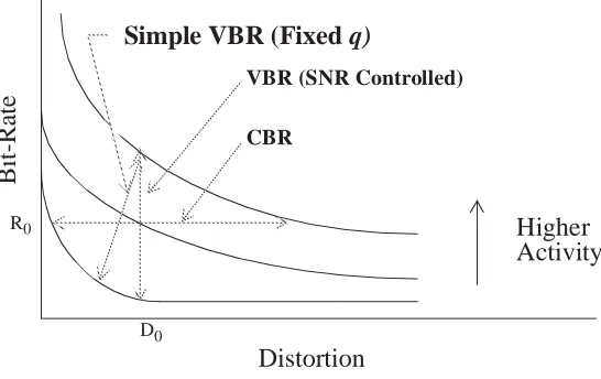
improve-ments in statistical multiplexing gain (SMG2). Figure 1 depicts the basic trade-off between distortion versus bit-rate for compressed video. We observe that distortion varies as an

encoder controls the rate (CBR), but if the encoder controls distortion (VBR), then

bit-rate varies. This behavior highlights the basic differences between CBR and VBR

encod-ing.

Increases in SMG occurs due to the fact that the likelihood of multiple bursty sources

simultaneously transmitting at their peak bit-rates is small. One of the first investigations

regarding the SMG of encoded video was done by Haskell, who found that a 2:1 gain was

achievable when multiplexing the outputs of several AT&T Picturephone encoders [10].

The SMG of VBR sources has been further quantified in early works by Kishino [24],

Morrison [38] and Verbiest [45], where gains of up to 4:1 were obtained for simple

sequences.

2. In the literature, definitions of SMG has arisen. One is the ratio of the multiplexer output link utilization for N VBR sources compared to only one source, given the same packet (cell) loss prob-ability. The second defines SMG as the ratio of the number of VBR sources to the number of CBR sources (preferably encoded using the same source material; however, this is often not the case and

AA AA AA AA AA AA AA AA AA AA AA AA AA AA AA AA AA AA AA AA AA AA AA AA AA AA AA AA AA AA AA AA AA AAA AAA AAA AAA AAA AAA AAA AAA AA AA AA AA A A AA AA AAAA AAAA AAAA AAAA AAAA AAAA AAAA AAAA AAAA AAAA AAAA AAAA AA AA B it-R ate Distortion Higher Activity R₀ D₀

Figure 1. Distortion versus bit-rate curves for compressed video. VBR (SNR Controlled)

AAA AAA AAA AAA AA AA AA AA AA AAAA AAAA AAAA AAAA AAAA AAAA AAAA AAAA AAAA AAAA AAAA AAAA AAAA AAAA AAAA AAAA AAAA AAAA AAAA AAAA AAAA AAAA AAAA AAAA AAAA AAAA AAAA AAAA AAAA AAAA AAAA AAAA AAAA AAAA AAAA AAAA AAAA AAAA AAAA CBR AA AA AAA AA AA AA A AAAA AAAA AAAA AAAA AAAA AAAA AAAA AAAA AAAA AAAA AAAA AAAA AAAA AAAA AAAA AAAA AAAA AAAA AA AA AAA AAA AA AA AA A A AA AA AA AA A A AAAA AAAA AAAA AAAA AAAA AAAA AAAA AAAA AAAA AAAA AAAA AAAA AAAA A A A A A A A A A A A A A

Simple VBR (Fixed q)

One drawback to multiplexing VBR sources is the increased possibility of packet loss.

Such losses result when multiple independent VBR sources cause the multiplexing buffer

to overflow. Analyzing the multiplexer buffer occupancy behavior is a major concern for

researchers. Simulation studies are often used in order to quantify the amount of loss,

since analytic methods are often intractable. In order to run these simulations, source

mod-els are used to provide input stimulus to the system under study. While actual video traces

may be used in place of a source model, this limits the input to a finite realization of the

underlying stochastic process, which reduces the generality of the simulation results.

In this paper, we survey statistical source models for VBR video which have been

pro-posed for both video conferencing and movie sequences. We define video conference

models as those being encoded using either H.261 or MPEG without B frames. A movie

sequence is one which is encoded using MPEG with I, B and P frames. Some examples of

models presented for movie sequences are: Star Wars,3 Last Action Hero,4 and The Wizard of Oz.5 Only MPEG-1 models were covered in this survey since a viable MPEG-2 model had not been published by the time this survey was concluded. For the most part, the

mod-els covered in this survey should apply to MPEG-2 equally as well. For introductory

mate-rial on the encoding standards H.261 and MPEG-1, refer to [31] and [28], respectively.

The motivation underlying the choice of these particular models is to present a

repre-sentative sampling of current VBR source models. The models are grouped into four

cate-gories (AR/Markov, TES, Self-Similar, Analytical/i.i.d.) and then presented in

chronological order. This was done so that the evolution of VBR modeling was readily

discernible. We provide detailed descriptions of each model, where necessary, and discuss

the motivations and merits of each model. We also describe how each model was validated

and the number of parameters used by the model.

The paper is organized as follows. Section 2 discusses on statistical modeling and

model validation. Section 3 covers models based on Markov Chains and Autoregressive

processes (AR). Section 4 covers models based on the TES process. Section 5 describes

models based on self-similar processes. Section 6 presents analytical and non-Markovian

models which are based on i.i.d. processes. Section 7 summarizes the paper, including a

comparison of the number of parameters required by each model in this survey.

Recom-mendations and issues relating to model selection are also discussed, as well as

2 Statistical Modeling and Model Validation

A good model is one which can accurately predict performance measures (statistics) of

a stochastic system. For example, if the researcher is interested in the cell loss probability

for an ATM buffer with VBR sources, then a good source model is one which produces a

sample path which can accurately predict this performance measure, when the system is

simulated. In most cases the validity or “goodness” of a model is determined by

compar-ing model predictions (e.g. simulation statistics uscompar-ing the empirical data as the traffic

source) and the corresponding statistics using the model as the traffic source. It is possible

for a model to predict one metric accurately and another inaccurately. For example, a

model may provide accurate predictions for cell loss probability, and be inaccurate

pre-dicting mean cell delay. The researcher must decide beforehand what the desired system

metrics should be, and select a model which can accurately predict these metrics.

There are reasons to argue that the validation of a source model requires that its

distri-bution and autocorrelation function match well their empirical counterparts, while using

as few parameters as possible6. Typically, one tries to fit the empirical data with a classical distribution such as Log-Normal or Gamma, but whether or not a good fit is found, the

empirical distribution (say, histogram) is a good fit by default. A common method used to

match distributions is the QQ plot. Matching the autocorrelation function is a more

diffi-cult task. The autocorrelation function is a proxy for the temporal (linear) dependence

within a stochastic process. Generally, stochastic processes may be classified into three

types: independent, short-range dependent (SRD) and long-range dependent (LRD). An

independent source is always uncorrelated, i.e., is identically zero for positive lags; the

converse is false, namely, lack of correlation does not imply independence. If the

autocor-relation function is summable (e.g. when it decays exponentially fast), then it is referred to

as an SRD process, but if it is not summable (e.g., when it decays hyperbolically), then the

source is referred to as an LRD process. The requirement to use few parameters is

moti-vated by the fact that they must be estimated from the empirical data. Each estimate incurs

a certain amount of error which tends to reduce the accuracy of the model as the number

of parameters increases (although those errors may occasionally cancel out).

In this survey, we classify the models into two types: hierarchical and

non-hierarchi-cal. Models which capture scene changes explicitly are referred to as hierarchical models.

A scene change process aims to model the relative frequency of individual scene types

over longer time scale (minutes or hours) than the bit-rate process (milliseconds). Scene

changes occur when the mean of the bit-rate process changes significantly as a result of a

considerable change in picture content (camera cuts).

The parsimony of a model is determined by the number of parameters it requires and

its complexity by the amount of computer time and memory required to generate a sample.

Models which require many parameters generally require many calculations in order to

generate a sample, but there are exceptions (e.g., TES). On the other hand, some models

require few parameters, but take a long time to generate each sample, since each sample is

calculated from all previous samples (e.g. LRD and self-similar models). It is desirable to

develop a model of minimal complexity which provides sufficiently accurate predictions

3 Models Based on Markov Chains and Autoregressive Processes

We provide a brief review of Markov Chains and Autoregressive (AR) processes since

many of the VBR source models are based on them. Both processes incorporate temporal

dependence. AR processes, in most case, use Gaussian random variables, producing

sequences which are Normally distributed. Markov Chains, those achieving steady-state,

can produce a wide variety of distributions.

3.1 Review of Markov process

Models based on a Markov process use states to represent bit-rate regimes (roughly a

range of bit-rates of a video sequence). A stochastic process {X_k}, k=1,2,... with state

space S={1,2,3,...} is Markovian if for every n and all states i₁,i₂,...,where it

satis-fies the Markov property,

Simply put, the current state of a Markov process depends only on its previous state

and not on any additional previous states. A stochastic process is called a Markov Chain if

the state space is countably infinite or finite.

As an example, a continuous-time discrete-state Markov process behaves as follows: it

enters a state and remains there for an exponential period of time whose parameter λ_i

depends on the state i. At the end of this period, the process moves to a different state

gov-erned by the Markov property. Transitions between states are controlled by a transition

probability matrix; corresponding transition probabilities are estimated from the actual

video trace. Steady-state distributions, if any, are determined from the transition matrix.

For a more complete discussion of Markov Chains, see [18].

i_n∈S

Markov Chains are often used to modulate other processes such as Bernoulli, Poisson

or AR. The state of the Markov Chain represents a different set of parameters for the

par-ticular process. While in a parpar-ticular state, the model generates samples according to the

particular process (Bernoulli, etc.), at the specific parameter settings. This is done for a

period of time until the process switches to a different state, generating samples using a

different set of parameters. Models of this type are referred to as Markov modulated or

Markov modified models. Some examples of such models are the Markov Modulated

Ber-noulli Process (MMBP) and the Markov Modulated Poisson Process (MMPP). We will

show many examples of video models which use Markov modulation.

3.2 Review of autoregressive process

In an AR process, the current value is a function of a weighted linear combination of

past values. Formally, it is expressed as

where a₀ is called the intercept and {a₁,a₂,...,a_p} are AR coefficients, p is the order of the

AR process and e(n) are the residuals, commonly assumed uncorrelated and Normally

dis-tributed. The AR coefficients can be determined using the recursive Levinson-Durbin

algorithm [40, Appendix 2A]. AR processes of order p are denoted by AR(p). A special

case of (2) is the AR(1) process

where a₁ is the autocorrelation coefficient at lag-1 when the sequence is stationary. Note

that (3) can be seen as a continuous-state, discrete-time Markov process. A model of this

form was presented in [32].

x n( ) a₀ a_i

i=1

p

∑

+ x n( –i)+e n( ),

= (2)

The AR process is a special case of the autoregressive moving average process

(ARMA) which adds a moving average process (MA) giving

The ARMA process is typically stated as ARMA(p,q) where p is the order of the AR part

and q is the order of the MA part. Determining the coefficients, b_j, is a bit more involved

than an AR process and usually requires some form of spectral analysis. [9]

3.3 ATM cell-level model using ARMA

Grunenfelder, et al. [9] developed a model, from a four second video conference

sequence, for the ATM cell interarrival process from a video encoder using conditional

replenishment7. The model defined a fixed time interval of 64 slots, where 1 slot equaled the time to transmit a 36 byte cell. The random process, {X_i}, defined the number of cells

generated by the encoder within this interval, where

where is white noise. The parameters for the model were estimated from the long-term

mean, variance and autocovariance of the empirical sequence. The coefficients, h_k, of the

MA part were determined using Fourier analysis. The ARMA process was referred to as a

colored-Gaussian process with zero mean, unit variance which implies that the

autocorre-lation function is not from a pure Gaussian process.

7. Encoders using conditional replenishment only transmit the difference in the pixel areas between a reference and current frame. This is done using differential pulse code modulation (DPCM). Areas which do not change are run length coded (RLC). When this difference becomes

x n( ) a₀ a_i

i=1

p

∑

+ x n( –i) b_je n( )

j=0

q

∑

+

= (4)

X_i = g(αZ_i–m+Y_i+ν_i)

Y_i h_kε_i–k

k=–m 2⁄ m 2⁄

∑

=

α <1

(5)

In digital signal processing terms, the ARMA sequence is generated using the ARMA

filter with white noise as input. Since the original sequence is not a zero mean process, the

output of the filter, {V_i}, is transformed using a zero-mean nonlinearity (ZMNL) function,

g(.), of the form aV_i+b.

This model requires 10,003 parameters, (α,a,b,h₁,h₂,...h_10,000), where the MA

coeffi-cients cover approximately seven frames. Model parameters were estimated from four

sec-onds of video. This model can be viewed as modeling the video sequence at the sub-frame

layer (slice/GOB) and it matches the pseudo-periodic autocorrelation function, typical of

these sequences, quite well.

3.4 Video conference model using Markov Chain

Heyman, et al. [13] developed a frame level8 ATM model of a 30 minute video confer-ence sequconfer-ence with no scene changes and moderate motion. The model defines the

num-ber of ATM cells per frame, X_n, and the state of the Markov Chain, Y_n, where

9_{. The transition probability matrix, P=[p}

ij], was estimated using,

This model requires many parameters due to the transition probability matrix. In order

to reduce the number of parameters, the authors used the Discrete Autoregressive Process

(DAR) which estimates the transition probabilities by using the empirical marginal

distri-bution and autocorrelation coefficient. The transition matrix is given by

8. The frame level corresponds to MPEG or H.261 pictures.

Y_n = X_n⁄10

p_ij number of transitions from state i to state j

number of transitions out of state i ---.

= (6)

where ρ is the autocorrelation at lag 1, I is the identity matrix, and each row of Q consists

of the marginal probability distribution function (pdf) of the empirical data. Since the

empirical data was found to fit a negative-binomial distribution, each row in Q contained

the probabilities defined by,

where the parameters r and p are estimated from the empirical data, and K is the maximum

number of cells in a frame. By using DAR the number of parameters was reduced to only

four: peak, mean, variance, and autocorrelation at lag 1.

Interestingly, this model gave rise to better bit-rate predictions than a second order AR

process which was also proposed at the time. This model is suitable for video conferences

with no significant scene changes, since it does not model the scene changes explicitly.

The model does rely on the use of a classical distribution (negative-binomial) in DAR;

however, the empirical distribution could be used.

Lucantoni, et al. [27] proposed a model using a discrete-state, continuous-time

Markov Renewal Process (MRP), which they compared to the DAR model. This model is

of the same vein as MMPP, but instead the bit-rate is fixed, not probabilistic. They divided

the range of possible rates into 40 equidistant levels and assigned a state in the Markov

Chain to each level. One, and sometimes two, geometric distribution were fitted to sojourn

time at each level. Sample paths generated by the model are strikingly similar in

appear-ance to the empirical trace data. They compared the leaky bucket contour curves,

gener-ated using both models, and found that MRP was better than DAR in approximating the

results produced when using the empirical sequence.

f₀, , , ,f₁ … f_K f_Kc

( )

f_k k+ +r 1 k

 

 _pr

1–p

( )k

=

f_Kc f_k

k>K

∑

=

3.5 Hierarchical model using composite AR processes and Markov Chain

Ramamurthy and Sengupta [41] proposed a hierarchical model which uses a Markov

Chain to capture the effects of a scene change. The model consists of two AR processes

where the first attempts to match the autocorrelation function at short lags and the second,

the autocorrelation at long lags. The third process is a Markov process which is used for

scene changes. Combining the three processes gives the final model

where

Equation (10) is used to generate a sequence whose autocorrelation function matches

that of the emprical sequence at short lags while (11) matches it at long lags. Bothh

equa-tions are AR(1) processes, where A_i and B_i are normally distributed with means: µ₁, µ₂

and standard deviations: σ₁, σ₂. Equation (12) is used to generate the extra bits needed

when a scene change occurs, where K_i represents the state of the Markov Chain and C_i is a

normally distributed random variable whose mean and variance depends on K_i. The

num-ber of parameters required for C_i is reduced from four to two by making the mean and

variance a function of α and β, where µ=α, σ=β when K_i=2 and µ=α/2, σ=β/2 when

K_i=1. The basic premise behind the use of the Markov Chain, shown in Figure 2, is to

generate the extra bits needed in the two frames following a scene change. We will see

later a model proposed by Heyman and Lakshman which also takes into consideration the

T_i = X_i+Y_i+Z_i (9)

X_i = a₁X_i–1+A_i, (10)

Y_i = a₂Y_i–1+B_i and (11)

first two frames after a scene change. This model requires a total of eight parameters

(a₁,µ₁,σ₁,a₂,µ₂,σ₂,α,β).

3.6 MPEG frame and slice layer models using Markov Chains

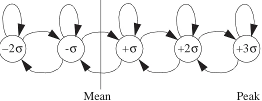
Pancha and El Zarki [39] proposed an MPEG frame and slice layer Markov Chain

model for a 3 minute, 40 second sequence of the movie Star Wars. This model differs

from Heyman’s model in that rather than each state representing the number of cells in a

frame, each state represents a bit-rate change of one standard deviation. This is illustrated

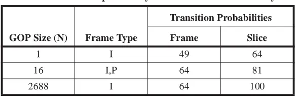
in Figure 3. Transition matrices were given for different GOP sizes and, in general, the

larger the GOP size the more states required in the Markov Chain. Also, the slice layer

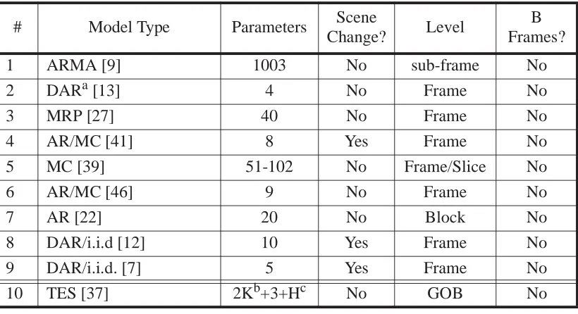
required more states than the frame layer. The number of parameters required by the

mod-els ranged from 51 for the frame layer to 102 for the slice layer, where the mean and

stan-dard deviation was estimated from the empirical trace data and added to the number of

transition probabilities which we summarize in Table 1.

K_i=0 K_i=1 K_i=2

p 1-p

1 1

Figure 2. Markov Chain of scene change process.

C_i(µ=α,σ=β) C_i(µ=α/2, σ=β/2)

+σ +2σ +3σ

2σ

– -σ

Mean Peak

3.7 Video conference model using composite AR processes

Yegenoglu, et al. [46] analyzed a full-motion color video sequence of 500 frames

encoded by discrete cosine transform (DCT), differential pulse code modulation (DPCM)

and motion compensation. The picture resolution was 720x480 pixels with 16 bits per

pixel and the rate was 30 frames per second. The primary motivation of this model was to

produce a multi-modal probability density function (in this case, Gaussian). Previous

work indicated that the probability density functions of VBR video conference streams

appeared to consist of a combination of probability distribution functions; indeed the

model did produce a multimodal probability density function.

The model is based on an AR process whose parameters are modulated by a Markov

Chain. The model quantizes bit-rates into N levels where a quantization level loosely

cor-responds to a scene class. The Markov Chain defines the transition process between

quan-tization levels, where a single distinct AR(1) process is defined for each state of the

Markov Chain. When the bit-rate crosses a quantization level, the first frame of the new

quantization level is sampled from an i.i.d. Gaussian random variable.

The state of the Markov Chain at a particular time instant, t, is defined as x_t, where

signifies a state change has occurred. For each state, i, there are a unique set of

Table 1. Transition probability count for frame and slice layer models.

GOP Size (N) Frame Type

Transition Probabilities

Frame Slice

1 I 49 64

16 I,P 64 81

2688 I 64 100

coefficients which is used to determine the number of bits per frame, y_t, given by the

regressive relation,

where G(.) is a Gaussian random variable and a(i) is the autocorrelation coefficient at lag

one at state i. When a state transition occurs, a sample is drawn from ,

where the mean and variance of the bit-rate process is conditioned on the state of the

Markov Chain, i. The parameters for (13) are calculated using the following constraints

where

is the conditioned expected square difference of the bit-rates in adjacent frames. This

parameter allows for the empirical data to be characterized in one pass, rather than the two

passes it would have otherwise required. The values , and are estimated

from the empirical data.

y_t a i( )yt–1 G µ( ) σi ( )i

2

,

( ),

+

G(η( ) νi , ( )i ),

  

= if xt = xt–1 = i

if x_t≠x_t–1; x_t = i (13)

G(η( ) νi , ( )i )

a i( ) 1 D

2

i ( )

2ν( )i

---, –

= (14)

µ( )i η( )i D

2

i ( )

( )

2v i( ) ---,

= (15)

σ( )i 2 D2( )i 1 D

2

i ( )

4ν( )i

---–

 

 _,

= (16)

D2( )i = E y[( _t–y_t–1)2 x_t = x_t–1 = i] ₍₁₇₎

The probability density function, f_Y(y), of the number of bits per frame, y_t, is

approxi-mated by a combination of N Gaussian densities

where p_i is the steady-state probability of state i in the underlying Markov Chain.

Three states were used to represent the quantizations (0,44), (44,55) and (55,∞) kbits/

sec, resulting in good agreement between the distributions of the model and empirical data

using the Kolmogorov-Smirnov test. The model captured the first, second and fourth

moments of the actual data; however, the third moment in one particular state differed

sig-nificantly. This was due to the fact that the actual data was not symmetrical about the mean

beyond 55 kbits/sec.

This model requires a total of nine parameters, three for each quantization level

where i={1,2,3}. It is useful for video conference sequences with small

to moderate motion and scene changes. The tricky part is to determine the appropriate

quantization levels, a task that requires visual inspection of the empirical bit-rate

distribu-tion.

3.8 Block-based video conference model using AR processes

Jabbari et al. [22] developed a block-based bit-rate model of a video encoder which

adhered to the general MPEG syntax. The encoder differs from the recommended MPEG

implementation in that the resolution is CCIR (720x480 pixels/frame) instead of SIF

(360x240 pixels/field). Interlaced scanning is used, producing two fields for every frame.

In most aspects, the encoder is more similar to MPEG-2 than to MPEG-1. The statistics of

encoded blocks contained within I and P frames were estimated for a sequence of 350

fields (175 frames) (the model does not account for B frames). The model divides each

f_Y( )y p_if_{G(η( ) νi, ( )i )}( )y i=1

N

∑

= (18)

D2( ) ηi , ( )i ,v i( )

Type 0 blocks are encoded using DPCM and are used for sequences with very little

motion. Type 1 blocks use motion compensation on sequences containing moderate

motion. Type 2 blocks use DCT on sequences with high motion. I frames contain only

type 2 blocks while, P frames contain all three types.

The model consists of a vector-valued sequence

whose components represent the number of Type 0, 1 and 2 blocks in each frame, n is the

frame index and e_i(n) is a Gaussian random variable with mean and variance for

i=0,1 and 2. The determination of the parameters for (19) is involved and is not included

here; but details can be found in [22].

The average number of bits for block type i, within frame n, is given by

where c_i is the first order AR coefficient and g_i is a Gaussian random variable. This is used

to find the total bits per block type i within frame n given as

The final model for the total number of bits per frame, u_T(n), is therefore,

The model produced sample data which was shown to match the distribution of the

actual data well via a QQ-plot. However, the model was not used in the simulation of a

multiplexer and the autocorrelation function of u_T was not given. A total of 20 parameters

are required for this model, of which

x₀( )n = a₀x₀(n–1)+e₀( )n ,

x₁( )n = a₁x₁(n–1)+b₀x₀( )n +b₂x₂( )n +e₁( )n ,

x₂( )n = a₂x₂(n–1)+e₂( )n ,

(19)

µ_i σ_i2

r_i( )n = c_ir_i(n–1)+g_i( )n , (20)

u_i( )n = r_i( )xn _i( )n . i = 0 1 and 2, , (21)

are used for the number blocks per frame, and , i={0,1,2}, are used for the

num-ber of bits per block.

3.9 Hierarchical model using the DAR process

Heyman and Lakshman [12] proposed an ATM frame layer model for sequences

gen-erated using a DPCM codec (motion compensation was not used) consisting of three

dif-ferent stochastic processes: (1) Scene length, (2) Size of the first frame after a scene

change, and (3) Size of frames within a scene. Scene change boundaries were determined

using the second difference

where X_i is the number of bits in frame i. A scene change is defined to occur when ∆_i is

large and negative (m was heuristically determined). The scene change process was

deter-mined to be uncorrelated; consequently, matching the distribution was sufficient. The first

frame after a scene change was found to follow a different stochastic process since the

scene content completely changes causing the frame to be regenerated. It was found that

scene length distributions fit Weibull, Gamma and Pareto distributions well while the

number of cells within a scene change frame fit Weibull, Gamma, and in one case Normal

distributions (some sequences, however, did not appear to fit any distribution). The frame

following a scene change frame was generated using linear prediction of the form

where a and b are fixed coefficients and ε_ι is white noise.

a₀µ₀,σ₀,a₁,b₀,b₂,µ₁,σ₁,a₂,µ₂,σ₂

{ , }

c_i,µ_i,σ_i

( )

∆_i (Xi+1–Xi)–(Xi–Xi–1)

1

m

---- X_i–k

k=1

m

∑

---= (23)

Since the frame size within a scene is correlated, a Markov Chain was used where each

state represented the integer part of and the transition probability matrix was

parsi-moniously determined using DAR. Each row of the matrix Q consisted of the

negative-binomial probabilities of the process (refer to Section 3.4 on page 10). The

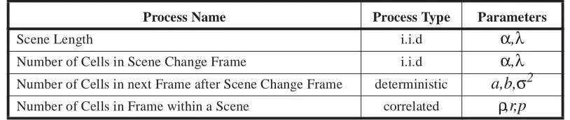
final model requires a total of ten parameters, which we summarize in Table 2.

Frater, et al. [7] proposed a similar model; however, the scene change boundaries were

determined in a slightly different way and processes for the first two frames after a scene

change were not considered. Scene change boundaries were determined by detecting a

large difference in the output of combination median, averaging filters. The scene length

pdf was found to be of the form

where a and b are constants, and n is estimated from the empirical sequence.

This model also used the DAR process and the negative-binomial distribution for the

frame size process; thereby, requiring a total of five parameters (ρ,r,p,b,n). Even though

the scene change frame process was not modeled, cell loss simulation results did appear to

match well the results produced when using empirical trace data.

Table 2. Process summary of hierarchical model.

Process Name Process Type Parameters

Scene Length i.i.d α,λ

Number of Cells in Scene Change Frame i.i.d α,λ Number of Cells in next Frame after Scene Change Frame deterministic a,b,σ2 Number of Cells in Frame within a Scene correlated ρ,r,p

X_i⁄50

X_i⁄50

{ }

p x( ) a

xn+b2

4 Models Based on the TES Process

TES processes are designed to fit simultaneously both the marginal distribution and

the autocorrelation function of the empirical data. It is a general method in that it can

match any marginal distribution exactly and simultaneously approximate a wide variety of

autocorrelation functions. A software package called TEStool supports TES modeling via

a graphical user interface which facilitates both algorithms and interactive searches for

TES models [14]. Recently, Jelenkovic and Melamed [23] have developed an algorithm

which largely automates the search process and invariably leads to a more accurate model

than those obtained via human interaction.

TES’s ability to match marginal distributions exactly and approximate many

autocor-relation functions makes it an excellent choice for constructing a source model. We give a

brief overview of TES processes; however, for more in-depth information, the reader is

referred to [35].

4.1 Overview of TES Process

TES defines a method for generating an auxiliary background process, {U_n}, which

allows one to vary the nature of dependence among the target random variables {X_n}. The

process {X_n} is referred to as the foreground process and is generated from {U_n} by using a

suitable transformation. The process {U_n} defines a random walk on the unit circle

(cir-cumference 1) based on the modulo-1 (fractional part) operator, defined as

10_.

x

Specifically, TES background processes come in two flavors, {U+} and {U_n- }, defined

as,

wherethe initial value U₀ is uniformly distributed on the interval [0,1) and {V_n}, called the

innovation sequence, consists of a sequence of i.i.d. random variables which are

indepen-dent of U₀. The background process {U+} can generate both negative decaying or

oscilla-tory autocorrelation functions while {U-} generates autocorrelations which alternate in

polarity between odd and even lags.

In general, {V_n} is obtained from the innovation density f_V, which is typically restricted

to step-functions in order to simplify the parameter search. In the simplest non-trivial case

of uniform innovations, {V_n} is determined by two parameters L and R where

is generally referred to as the single-step innovation function, Z_n are i.i.d. and uniformly

distributed on the interval [0,1) and . The parameterization (L,R) is

equivalent to the parameterization (α,φ) where

The (α,φ) parameterization is convenient for calculating the autocorrelation function. The

parameter α controls the magnitude of the autocorrelation function and φ controls its

oscil-lations.

Once the background process is determined, the next step is to define the desired

fore-ground process {X_n}. This is done by applying a transformation called the distortion

func-tion, to or . A common distortion is of the form , where is

U_n+

U₀,

U_n+_–1+V_n

〈 〉,

  

= U_n

-U_n+,

1–U_n+,

    

= (26)

n even

n odd n = 0

n>0

V_n = L+(R–L)Z_n. (27)

0.5

– ≤L< <R 0.5

α = R–L,

φ = R---._R+_–L_L

(28)

U_n+

the inverse of the cumulative histogram of the empirical data and is a stitching

trans-form. A stitching transformation is used, parameterized by a stitching parameter

where

is an intermediate step designed to “smooth” the sample paths of and

when crossing the origin. In most cases, a value at or near 0.5 is selected for ξ. Finally, the

requisite foreground TES sequence is defined by,

4.2 H.261 GOB video conference model using a TES process

Melamed, et al. [37] developed a model for the number of bits per group-of-blocks

(GOB) for H.261-encoded video. In H.261, each frame (352x288 pixels, Common

Inter-face Format, CIF) consists of 12 GOBs, each containing 33 Macroblocks. A Macroblock

contains four luminance blocks (block=8x8 pixels) and two chrominance blocks. The

sim-ulated system was an 802.3 LAN driven by multiple video sources. Each data packet

con-sisted of one or more GOBs.

They observed that the bit-rate data, at the GOB level, contained a significant periodic

component. The reason for this is that each GOB retains significant correlations between

the same blocks in successive frames since a block encodes the same portion of a frame

and scene content changes slowly over time (seconds). They removed this component

from the sample data, and then applied TES to the residual process, R_n. The periodic

com-S_ξ

0≤ ≤ξ 1

S_ξ( )y

y ξ

--1–y

1–ξ

---    

=

0≤ ≤y ξ

ξ≤y<1

(29)

S_ξ {U_n+} { }U_n

ponent was determined by using periodogram analysis to estimate the parameters K, ω_i, A_i

and B_i. These parameters are used to model the periodic component as

The residual process is then,

A single-step innovation density with α=0.50 and φ=0.30 was determined for R_n

(using the TEStool software) and the stitching parameter, , was set to 0.5. The periodic

process was added to the TES process yielding the final foreground process

The parameters for the model are then where i=1,2...K. The model

pro-duced an autocorrelation which matched its empirical data counterpart up to a lag of 100

frames. It then was compared to an earlier AR model which did not extract the periodic

component, but distributed the bits within a frame equally across GOBs. Simulation

showed the TES model produced lower packet loss and delay given the same throughput

when compared to results using the AR model.

4.3 Frame and Slice layer models using a generalized TES (G-TES) process

Lazar et al. [26] developed both a frame and slice layer models for a DCT encoded

version of the movie Star Wars. They used a generalized TES process in which the

innova-tion process is not i.i.d. Each scene was modeled as a stainnova-tionary process and scene lengths

followed a geometric distribution with parameter

P_n (A_icosω_in

i=1

K

∑

= +B_isinω_in). (31)

R_n = X_n–P_n. ₍₃₂₎

ξ

X_n = H_Y-1(S_0.5(U+_n))+P_n. (33)

α φ ξ, ,A_i,B_i

{ , }

p 1

1+E L[ ]_n

---,

where E[L_n]is the expected value of the duration of a scene, L_n. Scene change boundaries

were determined using the absolute difference in bit-rates of adjacent frames. The model

attempts to capture the large change in bit-rate magnitude observed at scene change

boundaries. The scene change process was incorporated into the innovation process as

where {Z_n} is a sequence of i.i.d. random variables with uniform marginals in the interval

[0,1), and {W_n} is a sequence of i.i.d. Bernoulli random variables signaling that a scene

change occurred. The GTES parameters were determined heuristically to be

and R=-L=0.001. The average scene length, E[L_n], was found to be about 100 frames.

The same innovation process, with only a slight modification, was used for the slice

layer model. In order to replicate the pseudo-periodic behavior of the autocorrelation

func-tion, they added a modulating function a_n. The background process was then defined as

where

with s being the number of slices per frame and % is the modulo operator.

The value of E[L_n] must now be expressed in terms of slices, so a scale transformation

changed it from 100 frames to 3000 slices (30 slices per frame). The parameters L and R

were set to 0.003 and 0.008 respectively, while α_cwas left intact.

The final model for both the frame and slice layer was

where a_n=1 for the frame layer model, and a_n is given by (37) for the slice layer model.

V_n (1–W_n)(L+(R–L)Z_n) W_n αc

2

---– +α_cZ_n

 

 _,

+

= (35)

α_c = 0.28

U_n = 〈U_n–1+a_nV_n〉, ₍₃₆₎

a_n

1 if 0 n%s s

2 ---–1,

≤ ≤

1 if s 2

---≤n%s≤s–1, –

    

= (37)

The parameters for the model are for the frame layer and

for the slice layer. The frame layer model matched the autocorrelation function of the

empirical data well up to a lag of about 300 frames, but thereafter it dropped below its

empirical counterpart. The slice layer model matched the autocorrelation well up to a lag

of 100 frames. The pseudo-periodic behavior was captured, but the model appeared to

underestimate the peaks in the autocorrelation function. The attractiveness of the GTES

approach, is that it provides a way to model VBR video at two different time scales (slice

and frame), while directly incorporating a scene change mechanism. This is the first model

considered to be of the hierarchical type. The model was used in simulations to determine

the bandwidth allocation required for sources of different service types.

4.4 MPEG Frame layer model using a composite-TES (C-TES) processes

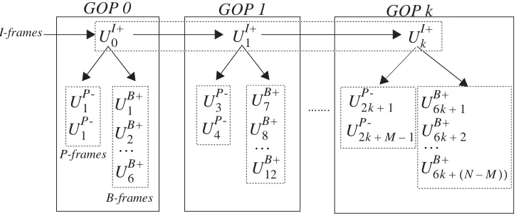
Reininger, et al. [42] developed a model for MPEG sequences containing I, B and P

frames. The model uses the background process for I, B frames and for P

frames giving the background sequences, , and . The scene change

process was not taken into account in this model.

An interesting point regarding this model is that the number of bits in B and P frames,

within a Group Of Pictures (GOP), depends on the I frame located at the beginning of a

GOP. Recall that in MPEG, a GOP consists of a set of I, B and P frames arranged in a

deterministic pattern which repeats throughout the sequence. For example, given a frame

sequence {...I₂B₃B₄P₂B₅B₆P₃B₇B₈I₃...} where the subscript is the index number of the

associated frame type, the background sequence variates for B₃ and P₂ are set equal to the

background sequence variate for I₂ . This makes intuitive sense,

because both B and P frames, within a GOP, reference the I frame in the encoding process.

An illustration of the relationship of the background sequences for I, P and B frames is

α_sα_c,ξ,p

{ , } { ,α_sα_c,ξ,p a, _n}

U+

{ } { }U

-UI+

{ } {UB+} {UP-}

U₂I+ = U₃B+ = U₂

The final model is composed of a deterministic combination of each frame type

pro-cess. Process selection is determined by the GOP frame sequence pattern, defined by the

MPEG encoding parameters N and M, which are the I frame and P frame distances

respec-tively. The three random processes are defined as,

The model requires nine parameters, , three for each frame type. One

point of interest here is that MPEG sequences with IBP frames exhibited a

pseudo-peri-odic autocorrelation function similar to that produced by slice layer sequences. This

behavior is caused by the deterministic sequencing of IBP frames and is captured well by

this model.

4.5 Frame layer model using a Markov modulated TES (MRMT) process

Melamed and Pendarakis [36] developed a model for a DCT encoded version of the

movie Star Wars (this is the same sequence used in Section 4.3) and takes scene changes

AAAAAAA A A A A A A A A A A A A AAAAAAA A A A A A A A A A A A A AAAAAAA A A A A A A A A A A A A A A A A A A A AAAAAAAA AA AA AA AA AA AA AA AA AA AA AA AA AA AA AA AA AA AA AA AAAA AAAA AAA AAA A A A A A A A A A A A AAAAAAA A A A A A A A A A A A A AAAA AAAA AAAA AAAA A A A A A A A A A A A A A A A A A A A A AAAA AAAA AAAA AAAA A A A A A A A A A A A A A A A A A A A

GOP 0 GOP 1

I-frames ... AAAAAAAAAAAAAAA A A A A A A A A A A A A AAAAAAAAAAAAAAA A A A A A A A A A A A A AAAAAAAAAAAAAAAAAAA AA AA AA AA AA AA AA AA AA AA AA AA AA AA AA AA AA AA AA AAAAAAAAAAAAAAAAAAA A A A A A A A A A A A A A A A A A A A GOP k

Figure 4. Generation of background processes for I, P and B frames in relation to the GOP sequence.

AAAAAAAAAAAAAAAAAAAAAAAAAAAAAAAAAAAAAAAAAAAAAAAAAAAAAAAAAAAAAAAAA A A A A A A AAAAAAAAAAAAAAAAAAAAAAAAAAAAAAAAAAAAAAAAAAAAAAAAAAAAAAAAAAAAAAAAA A A A A A A

U₁

P-U₁

P-U₁B+

U₂B+

U₆B+ …

U₀I+ U₁I+ U_kI+

U₃

P-U₄

P-U₇B+

U₁₂B+ U₈B+ …

U_2kP-₊₁

U_2kP-_+M–1

U_6kB+₊₁

U_6kB +_+(N–M)) U_6kB+₊₂

… P-frames

B-frames

X_nI+ H_Y I

1 –

S_ξ I Un

I+

( )

( ),

=

(39)

X_nB+ H_Y B

1 –

S_ξ B Un

B+

( )

( ),

=

X_nP- H_Y P

1 –

S_ξ P Un

P-( )

( ).

=

α φ ξ, ,

change process is not assumed to be i.i.d, but Markovian. The first task was then to

seg-ment the video sequence into individual scene segseg-ments and classify each segseg-ment. Scene

boundaries were detected by measuring the sustained absolute difference of the bit-rates

between a series of successive frames, again, similar to the technique was used in Section

4.311.

Once the video sequence is segmented, each segment is classified using a clustering

algorithm based on the minimum Euclidean distance between mean bit-rates. Four clusters

were sufficient to categorize the video sequence into four scene classes. A TES model was

then created for each scene class where each class was mapped to a state of a Markov

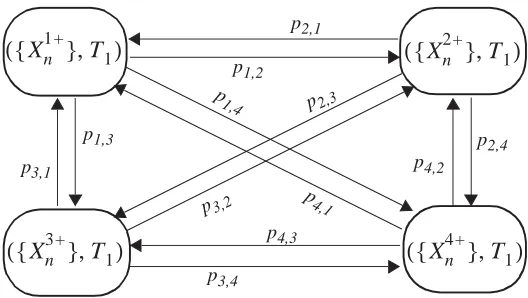
Chain, illustrated in Figure 5, whence the name Markov Renewal Modulated TES (MRMT)

process. Scene durations were class dependent; however, its autocorrelation function was

practically zero for lags greater than five frames, so it was assumed to be i.i.d. random

variable, represented by {T_i}, where i = 1,2,3,4 is the class index. Although it is not

explic-itly stated that the scene duration distribution is geometric, the video sequence is the same

as that used in [26] where its form is stated explicitly.

The final model consists of four TES processes, one for each class,

as well as four renewal processes for the corresponding scene durations.

The parameters for the model are , where i is the class index and

transition probability matrix. This yields 12 parameters for the matrix, and 3

for each TES process giving a total of 24 parameters. The model was used to generate

171,000 samples and the attendant sample path, histogram, autocorrelation function and

spectral density were compared to their empirical counterparts. In all cases excellent

11. It should be noted, that sequences containing I, B and P frames will require different methods to determine scene change boundaries. It seems feasible that, in this case, this technique could be

X_ni+ H_Y i

-1

S_ξ i Un

i+ (

( ) )

= i = 1 2 3 4, , , (40)

α_iφ_i,ξ_i,P

{ , }

matches were achieved. This model produced better matches to the autocorrelation

func-tion at long lags since the Markov Chain captures the longer-term scene change behavior.

p_1,2

p_2,4 p_2,1

p_3,1 p_1,3

p_4,3

p_3,4 p

1,4

p 4,1

p2,3

p3,2

Figure 5. The modulating Markov Chain which controls TES process selection and scene duration based on class type. Transition probabilities, p_ij, from class i to class j are determined from the empirical data of scene transitions. The amount of time spent in a particular state, T_i, is sampled from the empirical distribution of class i scene durations. {X_ni +} represents the TES process for scene class i.

p_4,2 X_n1+

{ },T₁

( )

X_n3+ { },T₁

( )

X_n2+ { },T₁

( )

X_n4+ { },T₁

5 Models Based on Self-Similar Processes

Loosely speaking, a process is said to be self-similar if the samples for that process

appears “similar”, regardless of the duration of the sampling interval (time scale). One of

the important characteristics of a self-similar processes is that it is long-range dependent

(LRD) which means that: (1) The autocorrelation function is not summable, (2) The power

spectrum at low frequencies is unbounded and approaches infinity as the frequency

approaches zero (DC component). This behavior differs from short-range dependent

(SRD) processes whose autocorrelation functions are summable and power spectrums are

bounded at low frequencies. Recent work by Beran, et al. [2] has shown that long-range

dependence is intrinsic to VBR sequences, and given that there is some evidence that LRD

processes can negatively affect multiplexing performance [1,30], source models which

capture this characteristic were developed. We present a brief overview of LRD; however,

for more information the reader should see [2].

5.1 Overview of Long-Range Dependence

It has been found that LRD processes occurs quite often in nature. Natural phenomena

such as rainfall, the annual growth of tree rings, river levels and discharges are often

described as self-similar processes. Hurst first discovered this property by investigating

the amount of storage required in the Great Lakes of the Nile river basin [17]. He found

that the expected value of the quantity (rescaled adjusted range statistic R/

S), asymptotically followed a power law

R n( )⁄S n( )

where c is a positive constant independent of n, is the adjusted range, is the

sample standard deviation, and H is the Hurst Parameter with range 0.5 < H < 1. The

rescaled adjusted range is calculated using

where

and X_i is the empirical sequence.

The value is calculated for different values of n and plotted in a Pox

diagram where is plotted on the y axis and is plotted on the

x axis. Linear regression is then used to estimate the Hurst parameter where

Typical values of H for various sequences are given in Table 3. Note that the value of

H for i.i.d random processes is 0.5, while for computer traffic it is approximately 1. Figure

6 shows the effect of the value of H on a random sequence. We plotted samples generated

using a fractional ARIMA process for four different values of H. We see that as H

increases, a noticeable low frequency oscillation is evident in the sequence envelope.

Once H is estimated, a processes such as Fractional ARIMA, or Fast Fractional

Gaus-sian Noise (ffGn) is used to create a background sequence, which may be used in turn to

generate the foreground sequence using the desired empirical marginal bit-rate

distribu-tion. Other methods can be used to estimate H in addition to R/S analysis such as

Vari-R n( ) S n( )

R n( ) S n( )

--- max 0 W( , 1,W2,…Wn)–min 0 0 W( , , 1,W2,…Wn)

S n( )

---= (42)

W₀ = 0,

W_k X_i–kX n( )

i=1

n

∑

= k = 1 2, , ,… n

(43)

E R n[ ( )⁄S n( )]

E R n[ ( )⁄S n( )]

( )

log log( )n

H logE R n[ ( )⁄S n( )] n

log

---.

5.2 Frame layer model using a fractional ARIMA (f-ARIMA) process

Garrett and Willinger [8] developed a model a DCT encoding of the movie Star Wars

Table 3. Hurst parameters of various traffic types.

TRAFFIC TYPE H

Computer Traffic [29] ≈1

CNN [4] 0.90

Star Wars (Motion JPEG) [4] 0.88

Star Wars (MPEG IBP) [4] 0.86

Star Wars (B/W, DCT) [8] 0.83

Video Conference [2] 0.6-0.75

i.i.d [6,33] 0.5

0 500 1000

−2 0 2 4 6 8 10 H=0.99

0 500 1000

−6 −4 −2 0 2 4 6 H=0.90

0 500 1000

−4 −2 0 2 4 H=0.70

0 500 1000

−4 −2 0 2 4 H=0.50

0 500 1000

0 0.5 1

H=0.50

0 500 1000

0 0.5 1

0 500 1000

−0.5 0 0.5 1

H=0.90

0 500 1000

−0.5 0 0.5 1

H=0.99

Figure 6. Comparison of the Hurst effect on random process (a) samples generated using fractional ARIMA process (x-axis = sample, y-axis = magnitude) (b) corresponding empirical autocorrelation functions (x-axis = correlation coefficient, y-axis = lag).

(a)

(b)

tribution they used a hybrid distribution, , which consisted of a concatenation of a

Gamma distribution for the left tail and a Pareto distribution for the right tail. Right tail

matching is particularly important because it describes the probabilities of high bit-rates

which can significantly affect queueing performance.

The model uses a fractional ARIMA(0,d,0) process to generate the background

sequence, where d=H-0.5, and its autocorrelation function is given by

The background process, {U_k}, is generated using Hosking’s algorithm12 [15] which is

an o(n2) algorithm. Each U_k is Gaussian with mean and variance which are given by

the function φ, defined recursively by

where

and the initial values are N₀=0 and D₀=1. The mean and variance is then

12. One interesting feature of this algorithm is that, given a discrete autocorrelation sequence, ρ_k, a sample path can be generated whose autocorrelation matches it. We will see this technique used

F_Γ⁄P

ρ_k d 1( +d)…(k–1+d)

1–d

( )(2–d)…(k–d)

---.

= (45)

µ_k σ_k2

φ_kj = φ_{k–1 j,} –φ_kkφ_{k–1 k, –j}, j = 1, ,… k–1 (46)

φ_kk = (N_k⁄D_k), ₍₄₇₎

N_k ρ_k φ_{k–1 j,} ρ_k–j,

j=1

k–1

∑

–

= (48)

D_k = D_k–1–(N_k2_–1⁄D_k–1). (49)

σ_k2

1–φ_kk2

( )σ_k2_–1

,

where the random variable, X₀, is sampled from a standard normal distribution. Finally,

the number of bits per frame is represented by the foreground sequence, {Y_k}, which is

generated using the transformation

where F_N is the standard normal cumulative distribution function and is the

inverse of the aforementioned hybrid Gamma/Pareto cumulative distribution function.

Note that the LRD property is still preserved when transforming from U_k to X_k.

The parameters required by the model are where and are the

mean and variance of the Gamma distribution and m_T is the slope of the line which best

fits the tail of the Pareto distribution. The model parsimoniously captures the LRD aspect

in this sequence using a single parameter.

5.3 Frame layer model using a fast fractional Gaussian Noise (ffGN) approximation

Enssle [5] developed a VBR model for an MPEG version of Star Wars containing I,B

and P frames. The model used the fast fractional Gaussian Noise (ffGN) algorithm to

gen-erate the background sequence. This method is an approximation to the fractional

Gauss-ian noise process and has a computational complexity of o(n). Consequently, ffGN

provides a faster way to generate the background sequence as compared to fractional

ARIMA.

The background process, {U_s(t)}, was generated using ffGN. The Hurst parameter, H,

was estimated to be 0.856, using Periodogram and R/S analysis, which compares well

with the value 0.83 found in [8]. The ffGN algorithm requires two additional parameters

besides H, called the base, B, and quality, Q. Selecting a value for B in the range

µ_k φ_kjX_k–j,

j=1

k

∑

= (50)

Y_k = F_Γ–1_⁄P(F_N( )U_k ). k>0 (52)

F_Γ–1_⁄P( ).

µ_Γ,σ_Γ,m_T,H

(This was heuristically determined). The background process, {U_s(t,H)}, consists of high

and low frequency components,

The low frequency component is a weighted sum of independent Markov-Gauss

pro-cesses,

The number of Markov-Gauss processes is

where n is the length of the time series and the weight factors are

The lag-1 covariance is given by

which is used in the Markov-Gauss process

where G_k(t) is standard normal.

U_s(t H, ) = U_l(t H, )+U_h(t H, ). (53)

U_l(t H, ) W_kG t r( , _k),

k=1

N

∑

= (54)

N = ln(Qn)⁄ln( )B , (55)

W_k H 2H( –1) B

1–H

BH–1

–

( )(B–2k 1( –H)) Γ(3–2H)

---.

= (56)

r_k e B k

–

–

= (57)

G t r( , _k)

G_k( )1 ,

r_kG t( –1 r, _k)+ (1–r_k2)G_k( )t ,

    

= (58)

t = 1

The high frequency component of (53) is

where G(t) is standard normal.

Each frame type has an corresponding distribution for the number of bits per frame,

which was determined to fit the Lognormal distribution well. The background process,

U_s(t,H), is then distorted using the transformation of the frame type distribution, , to

give

which translates to the following

where and i is the frame type I, B and P.

The model requires three parameters: B, Q and H for the background process and six

parameters: , , for the Lognormal distributions, for a total of nine

parame-ters. The model basically operates as follows. At time t, the frame type i, which is

prede-termined by the MPEG GOP pattern (IBBPBBP...), is used to select one of the three

transform functions: X_I(t), X_B(t) and X_P(t). A sample is then generated of {U_s(t,H)} which

is used in the selected transform function. Time is then incremented to determine the next

frame type and the process continues for the duration of the video sequence.

U_h(t H, ) 1 B

H–1

4 1( –H)Γ(–2H)

---– G t( )

= (59)

F_i–1

(60)

X_i( )t = F_i–1(U_s( )t ), i = 1 2, , ,… n

X_i( )t ln 1( +Φ)X_s( )t lnE X[ ]_i 1 2

---ln(1+Φ ) –

+ ,

exp

= (61)

Φ = (Var X[ ]_i )⁄E X[ ]_i 2

5.4 Frame layer SRD/LRD model using a f-ARIMA process

Huang, et al. [16] developed a model for an MPEG encoding of the movie Last Action

Hero, which contains I, B and P frames. It is referred to as a unified model because it uses

a hybrid function in order to match the autocorrelation function at both the short-term and

long-term lags. The Hurst parameter, H, was used to generate the LRD part of the

autocor-relation function, and a weighted sum of exponentials was used to match the SRD part.

These parts were then combined yielding the hybrid autocorrelation function

where K_t is the boundary between the SRD and LRD parts. The Hurst parameter was

determined using both R/S and Variance-time analysis and the SRD parameters were

determined by using regression analysis. Once the autocorrelation function was

deter-mined, Hosking’s algorithm was used to define the background process, {U_n}. Individual

histograms were constructed for each frame type and the attendant background process

was then transformed for each frame type via

Histograms were used since the authors determined that the empirical distributions did not

seem to fit any of the existing classical distributions.

The model requires four parameters to estimate ρ_k, the Hurst parameter H, and one

parameter for each cell in the frame type histogram. Samples were produced which

matched the autocorrelation function well for lags up to 500 frames. The portion of the

autocorrelation function up to lag K_t ~ 75 is fitted well by the exponential function. This is

probably the most accurate model to date in terms of matching the autocorrelation

func-tion for both short and long lags.

ρ_k e

0.00565k –

1.59k–0.2

  

= k<Kt

k≥K_t

(62)