Architecting a Workload-agnostic Heterogeneous Multi-core Processor.

(1)

ABSTRACT

WADHAVKAR, SALIL VIJAY. Architecting a Workload-agnostic Heterogeneous Multi-core Processor. (Under the direction of Dr. Eric Rotenberg.)

Improving single-thread performance still remains an important challenge. Heteroge-neous multi-cores offer the potential of improving single-thread performance by providing a number of core types that capture a wide range of application behaviors. Some prior approaches of choosing the constituent cores in a heterogeneous multi-core have focused on reducing power consumption by employing monotonic cores. Other approaches that aim to improve performance assume a priori knowledge of the workload. It is uncertain how such

workload-specificapproaches would perform if the workload changes in the future.

This dissertation addresses the question of choosing the cores in a heterogeneous multi-core in aworkload-agnosticmanner. The process of selecting the constituent cores is com-pletely independent of any benchmark suite. We present several approaches of choosing cores, and show that the resulting multi-core delivers high performance for a large number of application phases.

(2)

multi-core. Moreover, we demonstrate potential pitfalls of customization by showing that multi-cores tuned to a subset of the actual workload may perform poorly on the entire workload.

(3)

c

(4)

Architecting a Workload-agnostic Heterogeneous Multi-core Processor

by

Salil Vijay Wadhavkar

A dissertation submitted to the Graduate Faculty of North Carolina State University

in partial fulfillment of the requirements for the Degree of

Doctor of Philosophy

Computer Engineering

Raleigh, North Carolina 2012

APPROVED BY:

Dr. Eric Rotenberg Chair of Advisory Committee

Dr. James Tuck

(5)

DEDICATION

(6)

BIOGRAPHY

(7)

ACKNOWLEDGEMENTS

The last six years as a PhD student at NC State have been some of my most memorable years. Through times of difficulty, stress, and the general misery of grad life, many individuals have been a source of strength, courage, support and love, and have made this journey immensely fulfilling. These paragraphs represent a feeble attempt to show my gratitude to them in a rather clumsy form of expression, that is, language.

I would like to thank my parents for their unconditional love, encouragement, and support through the years. My achievements are a result of their nurture and the values they instilled in me. Their support and sacrifices will always motivate and inspire me to wholeheartedly pursue my dreams.

I have been very fortunate to work with my advisor, Dr. Eric Rotenberg. His ability to think deeply and critically, as well as articulate complex ideas with clarity has always inspired me. His passion for computer architecture has inculcated in me a strong work ethic of always doing my best, no matter how trivial the task. Most importantly, his encouragement and patience have taught me the value of persistence and diligence in accomplishing one’s goal. I am also grateful to him for providing me with financial support over the years.

I want to thank my committee members Dr. James Tuck, Dr. Huiyang Zhou, and Dr. Steffen Heber for their constructive feedback and comments. Their suggestions have been very valuable in improving my dissertation.

(8)

administrative support. I would like to thank them for quickly and smoothly processing all paperwork, especially close to deadlines.

This research was supported by NSF grant CCF-0811707 and gifts from Intel and IBM. Any opinions, findings, and conclusions or recommendations expressed herein are those of the author and do not necessarily reflect the views of the National Science Foundation.

My fellow CESR dwellers have been an exciting and intellectually stimulating group of people to work with. In addition to being wonderful colleagues, they have been good friends. I want to thank Niket Choudhary, Sandeep Navada, Muawya Al-Otoom, Elliott Forbes, Hashem Hashemi, Rami Al-Sheikh, Brandon Dwiel, Mark Dechene, Jayneel Gandhi, Hiran Mayukh, Tanmay Shah, and Rajeshwar Vanka for many brainstorming sessions, insightful discussions, and witty banter.

Outside of CESR, my friends have been a source of diversion during stressful times. Weekend get-togethers and the occasional poker nights with Jitendra Kumar, Pradeep Sharma, Adwait Bachuwar, Prabhakar Tembhurne, Shriraj Misal, Amit Naik, and Shreekanth Pavani are most memorable, and provided a much needed break from the monotony of grad life. Conversations and virtual hangouts with my college buddies Ninad Pradhan, Rahul Saxena, Raghvendra Cowlagi, and Robert Chettiar reminded me of life outside and beyond grad school.

(9)

(10)

LIST OF TABLES

Table 3.1 Design space parameters . . . 16

Table 3.2 Cores used for the validation of FabSim . . . 27

Table 3.3 SPEC SimPoints . . . 30

Table 3.4 MiBench SimPoints . . . 31

Table 4.1 G21 widths and cycle times . . . 33

Table 4.2 G21 cores . . . 35

Table 4.3 Cores of SQL-4 . . . 41

Table 4.4 Cores of FNILP-7 . . . 44

Table 4.5 Cores of ISOFREQ-4 . . . 47

Table 4.6 G21 subsetting strategies . . . 48

Table 4.7 The best homogeneous core and customized cores of theoutlier Sim-Points . . . 51

Table 4.8 Code behaviors and corresponding cores . . . 59

Table 5.1 Design space of kernels . . . 66

(14)

LIST OF FIGURES

Figure 3.1 IPC validation of FabSim . . . 28

Figure 4.1 Performance of G21 and Best-1 . . . 36

Figure 4.2 Speed of G21 over Best-1 for a different workload . . . 38

Figure 4.3 Performance of SQL-4 . . . 42

Figure 4.4 Performance of FNILP-7 . . . 45

Figure 4.5 Performance of ISOFREQ-4 . . . 47

Figure 4.6 C code from

gap.3229

. . . 52

mcf.2018

. . . 53

bzip.3089

. . . 55

gcc.473

. . . 55

Figure 5.1 Pseudocode corresponding to a pointer-chasing kernel . . . 62

Figure 5.2 Pseudocode corresponding to an array manipulating kernel . . . 63

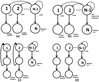
Figure 5.3 Kernel types and their structure. (a) Kernel type 0 (b) Kernel type 1 (c) Kernel type 2 (d) Kernel type 3 . . . 67

Figure 5.4 Percentage of distinguished kernels for different suitability thresholds 70 Figure 5.5 Classification tree for kernel type 0 . . . 73

Figure 5.6 Classification tree for kernel type 1 . . . 73

Figure 5.7 Kernel coverage for HCMP optimizing performance . . . 75

Figure 5.8 Classification tree for core 0.5W2 . . . 76

Figure 5.13 Performance of 59 SPEC SimPoints on a 5-core workload-agnostic heterogeneous multi-core . . . 79

(15)

Figure 5.15 Comparison of 5-Core workload-agnostic HCMP and custom HCMP

for 59 SPEC SimPoints . . . 81

Figure 5.16 Comparison of 5-Core workload-agnostic HCMP and custom HCMP for 40 MiBench SimPoints . . . 81

Figure 5.17 SimPoint coverage of custom HCMPs for 10 randomly selected SimPoints 84 Figure 5.18 SimPoint coverage of custom HCMPs for 15 randomly selected SimPoints 86 Figure 5.19 SimPoint coverage of custom HCMPs for 20 randomly selected SimPoints 86 Figure 5.20 SimPoint coverage of custom HCMPs for 25 randomly selected SimPoints 87 Figure 5.21 SimPoint coverage of custom HCMPs for 30 randomly selected SimPoints 87 Figure 5.22 SimPoint coverage of custom HCMPs for 35 randomly selected SimPoints 88 Figure 5.23 SimPoint coverage summary for custom HCMPs . . . 88

Figure 5.24 SimPoint coverage of custom HCMPs for 10 randomly selected Sim-Points without benchmark repetition . . . 89

Figure 5.30 SimPoint coverage for 100 randomly composed 5-core HCMPs . . . 92

Figure 5.31 Kernel coverage for HCMP optimizing performance . . . 92

Figure 6.1 Steering classification tree for core 0.5W2 . . . 95

(16)

Figure 6.7 Accuracy of random application steering mechanism for SPEC bench-marks . . . 100 Figure 6.8 Performance of application steering mechanisms for SPEC benchmarks100 Figure 6.9 Accuracy of application steering mechanism for 59 SPEC SimPoints . . 101 Figure 6.10 Accuracy of random application steering mechanism for 59 SPEC

Sim-Points . . . 101 Figure 6.11 Performance of application steering mechanisms for 59 SPEC SimPoints101 Figure 6.12 Accuracy of application steering mechanism for 40 MiBench SimPoints102 Figure 6.13 Accuracy of random application steering mechanism for 40 MiBench

SimPoints . . . 102 Figure 6.14 Performance of application steering mechanisms for 40 MiBench

Sim-Points . . . 102 Figure 6.15 Histogram of performance difference between consecutively ranked

(17)

CHAPTER

1

Introduction

Advances in circuit design technologies afford an increasing number of transistors to be ac-commodated on a single chip. The availability of these transistors has led to the wide-spread acceptance of the multi-core paradigm. Although increasing the number of cores allows multiple applications or threads to run simultaneously, the performance of single-threaded applications is largely unaffected. Moreover, chip power budgets impose a limitation on the number of cores active at a given time[1].

(18)

predictability, pattern of dependent and independent memory accesses, etc. These factors vary among applications making it difficult for a single core to capture this diversity. The single-ISA heterogeneous multi-core[2]paradigm offers a potential avenue to improve perfor-mance of single-threaded applications. Such multi-cores include differently designed cores that vary in pipeline depths, widths, structure sizes, cache memory sizes, clock frequencies, etc., tailored to different applications or classes of applications[3].

One approach for choosing the constituent cores is to use pre-designed cores belonging to different generations of processors[2]. This approach has the advantage of eliminating core design and verification effort by reusing existing designs. Although this method simplifies the process of choosing cores, it imposes a monotonic relationship among the cores and reduces the potential of the heterogeneous multi-core to deliver the highest possible performance. Moreover, such approaches aim to improve power and energy efficiency.

Other approaches[4][5]perform design-space explorations of core architectural parame-ters to identify per-application optimal cores. These cores are then used as a starting point to distill fewer cores. So far, approaches for choosing the non-monotonic cores have been

workload-specific. That is, those constituent cores are fine-tuned for the set of applications

(19)

workload altogether.

This dissertation addresses the question of choosing the cores in a heterogeneous multi-core in aworkload-agnosticmanner. The process of selecting the constituent cores is com-pletely independent of any benchmark suite. We present several approaches of choosing cores, and show that the resulting multi-core delivers high performance for a large number of application phases.

To gain further insight into the interaction of cores and application behavior, we take a systematic approach to model the diverse nature of instruction-level parallelism in ap-plications. Important core types can be suggested based on that analysis. We consider four broad classes of code structure and construct micro-kernels modeling that structure using synthetic code. These classes are: pointer-chasing, array manipulations, arbitrary serial and arbitrary parallel. These classes represent higher-level code behaviors that exhibit fundamentally different dependence relationships among instructions. This classification helps us narrow down higher-level code behavior to generic kernel templates. Along the lines of statistical simulation[6], we generate synthetic instructions based on these kernel templates, and evaluate their performance on a representative design space of cores. By varying different parameters of the kernel templates, such as the number of dependence chains, branch misprediction rate, cache miss rates, etc., we can control the amount and nature of instruction-level parallelism in the synthetic code.

(20)

space of cores, several kernels achieve high performance (within 90% of peak performance) on many diverse cores. Whereas, a comparatively smaller fraction of kernels achieves high performance on a small number of cores. We call kernels that exhibit marked performance differentiationdistinguishedkernels. Analyzing the distinguished kernels yields insight into specific core preferences of the kernels.

Our evaluation shows that a heterogeneous multi-core with 5 core types that is not tailored to any specific workload, delivers at least 90% of peak achievable performance for 94 out of 99 10 million instruction SimPoints from SPEC 2000 and MiBench benchmark suites. While it is theoretically impossible to study all possible code behaviors, we believe that our methodology covers a broad spectrum of instruction-level behaviors of single-threaded applications, and the workload-agnostic heterogeneous multi-core would be robust for other CPU-centric applications.

Steering an application to an appropriate core is an important consideration in hetero-genenous multi-core design. Analyzing the sample space of kernels shows how the kernel parameters and core choice are related. These insights can be leveraged in developing application steering mechanisms.

1.1

Contributions

(21)

we present G21 – a heterogeneous multi-core with 21 core types. The cores of G21 are chosen without anya prioriknowledge of the workload. By providing cores for a range of pipeline widths and frequencies, G21 provides broad microarchitectural diversity catering to a variety of ILP and MLP characteristics. The robustness of G21 and the diversity of its cores suggest that it may be usedin place of the entire design space if fewer cores are to be chosen.

• For a smaller number of core types, three additional approaches for robust design are also presented. The first approach is based on a well-established observation - the square-root law[7]. The second approach is based on the observation that some code sequences have several overlapping dependence chains with independent instructions close together (near ILP), whereas some code sequences are serial with independent instruction distant from each other (far ILP). The third approach attempts to simplify overall chip design by limiting all cores to the same clock frequency, although the core configurations may be significantly different. Although a few applications degrade noticeably, these approaches deliver close to peak performance with a smaller num-ber of cores types. These core types are also chosen without any knowledge of the applications, making them robust to any changes in the workload.

(22)

this sample space of kernels allows us to select cores that deliver high performance on a large proportion of the sample space. The key results of this study are:

– Our approach yields a 5-core workload-agnostic multi-core that delivers at least 90% of peak performance for 94 of 99 benchmark phases compared to 97 for the optimal 5-core multi-core customized for all 99 benchmark phases. For the benchmark phases that did not achieve 90% of peak performance, the average degradation on the workload-agnostic multi-core was 13% compared to 11% for the optimal multi-core.

– On average, the 5-core workload-agnostic multi-core performs within 98% of the optimal 5-core customized for all 99 benchmark phases.

– We show that customizing a heterogeneous multi-core for specific benchmark phases may lead to designs that perform poorly on unseen phases.

– We test the comprehensiveness of our kernel space by expanding the boundaries of kernel parameters as well as increasing their granularity to yield a kernel space almost 9 times the original. The original 5-core heterogeneous multi-core is the best 5-core design even for the larger kernel space. This increases confidence that the kernel space is representative of a broad spectrum of behaviors, and that the workload-agnostic multi-core is robust enough to deliver high performance on unseen applications.

(23)

choice of core. Statistical tools such as classification trees quantify this relationship, and are used as a starting point for application steering mechanisms.

1.2

Outline

The rest of this document is organized as follows.

Chapter 2 discusses the background and related work. Prior approaches for designing heterogeneous multi-cores are discussed.

Chapter 3 elaborates on the evaluation methodology. FabScalar[8]is used to obtain timing data and my contribution to the FabScalar project is detailed. Simulation and benchmark selection methodologies are also discussed.

Chapter 4 describes the design approaches for a workload-agnostic heterogeneous multi-core. The performance of G21 and of other workload-agnostic approaches are evaluated, and results are presented. Also, an analysis of benchmark phases is presented to understand the diversity in application characteristics and corresponding core preferences.

Chapter 5 presents a systematic exploration of instruction-level characteristics, and presents a methodology to obtain a robust workload-agnostic heterogeneous multi-core.

Chapter 6 describes an application steering mechanism based on analyzing the synthetic kernels.

(24)

CHAPTER

2

Related Work

There has been significant prior work relating to the design of heterogeneous multi-core processors. This chapter presents an overview of past related works and highlights the differences with the research presented in this thesis.

2.1

Selection of Cores

(25)

pre-viously implemented Alpha designs - EV4, EV5, EV6 and a single-threaded version of EV8 (EV8-). They focus on single-thread performance, assuming only one core is active at any time. All cores are clocked at the same frequency. This implies a monotonic performance ordering of cores from the simpler EV4 (least performing) to the most complex EV8- (highest performing). Their work differs from this thesis in several key aspects. Firstly, since the heterogeneous multi-core paradigm provides the freedom to design each core differently from scratch, this research considers an extensive design space of superscalar processors. Secondly, in this research, cores with different clock frequencies are considered, and the impact of propagation delay on core complexity is modeled using FabScalar[8]. This leads to non-monotonicity of core designs, that is, a wide-issue complex core with large structures may not always perform better than a narrow-issue simple core for all applications.

(26)

experiments with unconstrained power and area budgets, the largest and most complex core performs best overall, which is only true if all cores are forced to run at the same frequency. They achieve the benefit of heterogeneity through power and area constraints. Secondly, they perform exhaustive exploration of all multi-core combinations to recommend the best design. Further, as they mention, their methods are chiefly applicable in embedded multi-processor systems where the workload is usually known.

Morad et al[10]perform theoretical analysis of homogeneous and heterogeneous multi-cores to obtain upper bounds on performance for multi-threaded applications. They propose executing serial parts of multi-threaded applications on complex cores and parallel parts on several simpler cores. They conclude that heterogeneous multi-cores can achieve higher performance than homogeneous multi-cores for similar power budget. In a similar vein, Sule-man et al[11]leverage the heterogeneous multi-core substrate to accelerate multi-threaded applications by executing critical sections on a complex processor.

Lee et al[4]explore a large design space of cores to identify per application optimal energy-efficient processors. To speed up the design space exploration, they formulate regression models to estimate the performance of different cores on different applications. In order to reduce the number of cores in a heterogeneous multi-core, they employ K-means clustering to identify “compromise” cores. Similar to most prior work, their scheme relies on knowledge of the workload to recommend core designs for a heterogeneous multi-core.

(27)

increased logic complexity on clock frequency. However, similar to most other prior work, their recommendations for optimal multi-core designs also depend on the knowledge of workload. Architectural contesting[12]leverages the heterogeneous multi-core paradigm to improve single-thread performance by running the application redundantly on two (or more) cores designed for different behaviors. The faster core broadcasts the results of execution to the slower cores. Because of execution redundancy, optimum performance is always achieved. The selection of these “contesting” cores is done by finding the performance optimal cores for all benchmarks using design space exploration. Fewer core types are then distilled from this palette of per application optimal cores and employed for contesting.

Along similar lines of this research, Patsilaras et al[13] also leverage a heterogeneous multi-core substrate to include specialized cores for speeding up applications that exhibit significant memory-level parallelism.

2.2

Statistical Simulation

(28)

design space explorations of superscalar processors.

2.3

Application Steering

(29)

CHAPTER

3

Evaluation Methodology

(30)

physical design, or Register-Transfer Level (RTL) descriptions of the processor is required. This thesis leverages FabScalar[8], which can provide synthesizable physical designs of an arbitrary superscalar processor.

To obtain the performance of a processor, microarchitects generally simulate different applications (or benchmarks) for that design using a cycle-level simulator. A cycle-level simulator typically models the activity for various structures of the processor at every cycle. The accuracy of the performance estimated by the cycle-level simulator depends on how closely it models the simulated structures. This thesis contributes to the FabScalar project by developing a highly detailed cycle-level simulator, FabSim, that models every structure of a given design accurate to the RTL description.

The rest of the chapter describes the construction of the design space, provides a detailed description of FabSim, and describes the benchmarks used to performance evaluation.

3.1

Design Space

(31)

480 points using simulations since they vary architectural parameters at a coarse-grained level. Lee and Brooks[22]explore a design space of 240 billion points using regression models since they vary architectural parameters at a fine level and assume that every possible core configuration represents a valid design. Therefore, in order to draw meaningful conclusions from results and provide context to them, it is important to describe the core design space in detail.

In this research, FabScalar[8]generated designs populate the design space. FabScalar provides the facility to generate synthesizable RTL designs of an arbitrary superscalar config-urations within the limits of its Canonical Pipeline Stage Library (CPSL). Synopsis Design Compiler and the FreePDK standard cell library[24]are used to obtain logic delays. Cache latencies are obtained using Cacti[25]. Because performance is a function of the microarchi-tectural configuration and technology, any conclusions drawn from technology-dependent research, such as this and other prior work, would need to be re-evaluated if different tech-nology is used.

(32)

Table 3.1: Design space parameters

Parameter Range Total

Clock period (ns) 0.5 :: 0.1 :: 1.2 7

Fetch/dispatch width 2 :: 1 :: 8 7

Issue/retire width 2 :: 1 :: 8 7

Issue queue size 16,24,32,48,64,96,128 7

Reg file size 64,128,192,256,384,512 6

Load(/store) queue size 8,16,24,32,48,64 6

ALU mix 10

D$ size 8,16,32,64,128 5

I$ size 8,16,32,64,128 5

Total 21.6 million

3.2

Realistic Pruning of the Design Space

A superscalar processor pipeline is considered balanced if the delays of each stage are identi-cal (or have insignificant differences). A balanced pipeline represents an optimal distribution of logic for the given degree of complexity. However, real logic cannot be arbitrarily parti-tioned into chunks with identical delays. A pipeline stage consists of logic and hardware structures that are typically divided to perform specialized functions. Thus, certain locations in the stage are more suitable for pipelining due to this inherent separation by function. Also, hardware structures like RAMs cannot be partitioned to obtain an arbitrary division of delay.

(33)

is not sub-pipelined. The delay of the fetch stage stage may be non-trivially different from the delay of the issue stage, despite adjusting structure size and complexity to minimize this difference. The imbalance, in this case, is at the canonical stage level. Second, consider the sub-pipelining of one of the canonical stages for a given complexity. The issue stage, for example, can be pipelined into three sub-stages[26] by placing pipeline registers at appropriate boundaries. Doing this, however, divides the total issue logic delay unevenly.

(34)

3.3

FabSim: The Cycle-accurate FabScalar Simulator

Cycle-level processor simulators (also known as timing simulators) are widely used in academia and industry. SimpleScalar[27], SESC[28], PTLsim[29], etc are some examples of popular academic processor simulators. A cycle-level simulator is an indispensable tool for quickly evaluating microarchitectural ideas. One of the first steps to quantify the benefit of a microarchitectural optimization is to evaluate it on a cycle-level simulator. Cycle-level simulators are typically written in a high-level language such as C, C++or Java. This makes them easier to extend and much faster than Register Transfer-Level(RTL) simulators. For example, if a researcher wants to test a novel load speculation scheme, he/she can evaluate its performance impact by modeling it in a simulator, without the need to develop any detailed hardware models. In microarchitecture research, insight and understanding of many hard-ware mechanisms is derived from the results of a cycle-level simulator. It is, therefore, very important that the simulator model the underlying microarchitecture in considerable detail. Approximate or inaccurate modeling of branch misprediction penalties or key hardware such as the instruction fetch engine and the instruction issue logic may lead to wrong conclusions.

(35)

simulating 100 million instructions on the RTL model of a processor takes several hours. Accurately measuring the impact of any microarchitectural optimization requires developing detailed RTL models and significantly increases design time.

The objective of FabSim is to be cycle-accurate to an RTL model of any processor com-posed from FabScalar’s canonical pipeline stage library (CPSL)[8]. Since FabSim is written in C++, it is orders of magnitude faster than full RTL simulation. At the same time, FabSim’s design approach ensures that its performance results closely match those produced by full RTL simulations. FabSim also includes a functional checker that independently and func-tionally executes instructions. At the time of instruction retirement, results from FabSim and the functional checker are compared to ensure functional correctness of FabSim.

3.3.1

Canonical Interfaces

A unique feature of the FabScalar CPSL is the canonical definition of the pipeline stage interfaces. This predetermined definition at the canonical pipeline stage level allows for multiple flavors of implementation for the pipeline stages. At the top level, these interfaces remain fixed (for given pipeline widths) and hide the underlying implementation (variability in pipeline depths), essentially treating them as black-boxes.

(36)

to aid debugging. Each pipeline stage is defined as an interface only C++abstract base class. This allows several implementations of a pipeline stage that all adhere to the same interface, making FabSim very flexible and easy to use. Each implementation of a pipeline stage is derived from the respective base interface class. The implementation (or derived class) contains its own structures and logic. A researcher using FabSim can replace any of the canonical implementations with his/her own without requiring any changes to the rest of the simulator, so long as the pipeline stage interfaces are obeyed. For example, a researcher can easily replace the stock fetch stage with an implementation that models complex branch-prediction techniques such as L-TAGE[30]or EXACT[31][32].

Some of the interface functions that are common to most pipeline stages are briefly mentioned below.

clock_edge(): Clocks the register-based structures.

pipeline_stage(): Evaluates the actual logic pertaining to the pipeline stage.

read_instructions(): Reads the output instructions of the pipeline stage.

read_ready(): Reads the ready signal.

write_stall(): Writes a stall signal so clocked structures do not update their values.

write_flush(): Writes a flush signal so clocked structures are reset.

(37)

Apart from these functions, a pipeline stage may have other interfaces that are specific to the logic of that stage. Also, a pipeline stage may interact with another stage that is not immediately preceding or following it. Such logic warrants special interface functions. For example, when instructions retire, the retire stage communicates the names of physical registers that are unmapped and should be added to the physical register free list. In this case, a special interface function is needed for communication of such information. Note that most of these special interface functions only pertain to the general structure of a canonical superscalar processor. These interface functions are not typically attached to any specific implementation of the underlying logic. If an alternate implementation of a canonical pipeline stage requires non-canonical transfer of data (thus, additional interfaces) then changes to the canonical interfaces are necessary. This unavoidable result is simply an artifact of the modification of the canonical superscalar template which would require modifications to the interfaces of the FabScalar CPSL too.

(38)

3.3.2

Modeling of Clocked Structures

An important factor to consider when modeling hardware in a cycle-accurate manner is the software implementation of clocked structures. In hardware, clocked structures such as pipeline registers are implemented as edge-triggered flip-flops. Other structures such as the rename map table or the re-order buffer are implemented as custom RAMs. These structures are different from combinational logic in that they are synchronously updated only on clock edges. It is only on a clock edge that the input data to a clocked structure (e.g. pipeline register) is transferred to the output. Between two consecutive clock edges, the combinational logic in the core processes the unchanging output of registers and sets up their the inputs.

In an RTL simulation, the outputs of pipeline registers and other clocked structures define the microarchitecture-level pipeline state. A true cycle-accurate software simulator must match the pipeline state on every cycle of a corresponding hypothetical RTL simulation. It is thus very important to model the clocked structures very accurately.

FabSim takes the approach of literally modeling pipeline registers. Each simulated register object has interfaces for writing the input data, stall and flush signals, reading the output data, and modeling the clock edge. When data and control signals are written to a register object, they are buffered. Output is updated only in the

clock_edge

method based on the

stall

and

flush

signals. This ensures that the behavior of clocked structures is modeled

(39)

3.3.3

Modeling pipeline depth

The FabScalar canonical superscalar template delineates the processor pipeline at canonical stage boundaries. Internal logic details of a specific implementation of a pipeline stage are not important at the canonical stage boundaries. Since FabSim needs to be cycle-accurate at the canonical stage boundaries, internal implementation is simplified. The FabScalar CPSL provides various flavors of pipeline stages with different degrees of pipelining. For example, the decode stage has three variants with sub-pipe stage depths of 1, 2, and 3. A depth of 1 implies that all the logic in the decode stage, that is instruction decode, cracking into micro-ops, and writing into the instruction queue, is processed in one cycle. On the other hand, a depth of 3 separates the same overall logic into the three aforementioned chunks and inserts pipeline registers in between. For a depth of 2, a pipeline register is inserted before the fetch queue. However, at the top level, the canonical behavior of the decode stage does not change. FabSim leverages this observation to simplify the modeling of different depths. Since the total amount of logic to be processed does not change, FabSim processes it all together. However, FabSim adds an appropriate number of dummy pipeline registers

afterthe logic to provide the effect of sub-pipelining. In this manner, FabSim maintains

cycle-accuracy at the canonical boundaries, despite not modeling partitioning of internal logic exactly.

(40)

different configurations[26]. A configuration of (X,Y) means wakeup-select loop depth of X and total issue depth of Y. To model a sub-pipelining configuration of (1,1), no intermediate pipeline registers are necessary. However, to model a sub-pipelining configuration of (2,3), pipeline registers must be placed at specific logic boundaries. Simply inserting two or three dummy registers at the end of the issue stage actually results in a configuration of (2,2) or (3,3) respectively. This breaks FabSim’s cycle-accuracy since the logic is not correctly represented. Therefore, FabSim models such logic in precise detail in order to maintain cycle-accuracy at the canonical boundary.

3.3.4

Simulator Optimizations and Features

One of the benefits of high-level language cycle-level simulator is that it provides a researcher with the ability to quickly evaluate the potential of ideas through limit studies, without requiring a thoroughly worked-out hardware solution. This level of flexibility is difficult, if not impossible, to incorporate in a simulator that very accurately models real hardware. Still, FabSim provides some features that are useful in deriving upper performance bounds for microarchitectural ideas.

For example, the FabScalar CPSL specifiesfourbasic types of instructions:simple,

com-plex,branchandmemory. Each instruction type has a dedicated ALU type that can only

(41)

support multi-function ALUs that can execute a simple, complex or branch type instruction. Further, for a given issue width, each ALU can be individually configured to support the execution of any combination of the three instruction types. Memory instructions require a dedicated issue port due to significant differences in the way memory instructions are executed. Another example of a feature that is difficult to implement in real hardware is an oldest-first instruction select/issue policy. FabSim does not currently such a policy, but it can be extended to do so without significant difficulty.

FabSim models microarchitectural structures in very fine detail. Most cycle-level sim-ulators used in academia do not exhibit such depth and accuracy in modeling hardware. Unsurprisingly, increasing the level of detail incurs a significant cost in speed of simula-tion. FabSim executes at a fairly slow speed of 10’s to 100’s of KCPS (kilo cycles per second). However, FabSim is about 10x faster than an equivalent RTL simulation.

3.3.5

FabSim

/

RTL co-simulation

Recall that the goal of FabSim is to match an RTL simulation at the canonical pipeline stage boundaries. This enables the possibility of tightly coupled FabSim/RTL co-simulation. Since FabSim is written in C++, it can be compiled with the RTL (Verilog) models using

Verilog Procedural Interface(VPI). A VPI is used to invoke C/C++code from within a Verilog

(42)

Thus, FabSim’s combination of cycle-accurate performance reporting, fast simulation compared to RTL, as well as a fair degree of flexibility make it a useful and versatile tool in the FabScalar framework. The possibility of FabSim/RTL co-simulation also adds to its utility.

3.3.6

Validation of FabSim

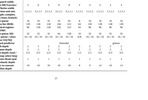
To demonstrate the accuracy of FabSim, RTL descriptions for 10 cores were obtained from FabScalar. These RTL descriptions correspond to the physical designs of the 10 cores. Table??

(43)

Table 3.2: Cores used for the validation of FabSim

Core-1 Core-2 Core-3 Core-4 Core-5 Core-6 Core-7 Core-8 Core-9 Core-10

Fetch/Decode/Rename 4 4 5 6 8 2 4 4 4 4

/Dispatch width

Issue/RR/Execute/ 4 6 5 6 8 4 4 4 4 4

WB/Retire width

function unit mix 1,1,1,1 3,1,1,1 2,1,1,1 3,1,1,1 5,1,1,1 1,1,1,1 1,1,1,1 1,1,1,1 1,1,1,1 1,1,1,1

(simple, complex, load/store, branch)

fetch queue 16 16 32 32 64 8 16 16 16 16

active list (ROB) 128 128 128 256 512 64 128 128 128 128

physical register 96 128 128 192 512 64 96 96 96 96

file (PRF)

issue queue (IQ) 32 32 32 64 128 16 32 32 32 32

load queue/store 16/16 16/16 16/16 16/16 16/16 8/8 16/16 16/16 16/16 16/16

queue (LQ/SQ)

branch predictor bimodal gshare

Fetch depth 2 2 2 2 2 2 2 2 2 2

Rename depth 2 2 2 2 2 1 2 2 2 2

Issue depth: total/ 2/2 2/2 2/2 2/2 2/2 1/1 1/1 3/2 2/2 3/2

wakeup-select loop

Register Read (and 1 1 1 1 1 1 1 4 1 4

Writeback) depth

fetch-to-execute 10 10 10 10 10 8 9 14 10 14

(44)

Figure 3.1 shows the IPC from both simulations for the six benchmarks. It is clearly seen that the IPC estimated by FabSim (indicated as “C”++”) very closely tracks the IPC obtained through a full RTL simulation (indicated as “Verilog”). This shows that FabSim is accurate enough to be used in lieu of RTL simulations.

Performance trend - bzip

0 0.2 0.4 0.6 0.8 1 1.2 1.4

1 2 3 4 5 6 7 8 9 10

Cores

IPC

Verilog C++

Performance trend - gap

0 0.1 0.2 0.3 0.4 0.5 0.6 0.7 0.8 0.9 1

1 2 3 4 5 6 7 8 9 10

Cores

IPC

Verilog C++

Performance trend - gzip

0 0.1 0.2 0.3 0.4 0.5 0.6 0.7 0.8 0.9 1

1 2 3 4 5 6 7 8 9 10

Cores

IPC

Verilog C++

Performance trend - mcf

0 0.1 0.2 0.3 0.4 0.5 0.6 0.7 0.8 0.9 1

1 2 3 4 5 6 7 8 9 10

Cores

IPC

Verilog C++

Performance trend - parser

0 0.1 0.2 0.3 0.4 0.5 0.6 0.7 0.8 0.9 1

1 2 3 4 5 6 7 8 9 10

Cores

IPC

Verilog C++

Performance trend - vortex

0 0.2 0.4 0.6 0.8 1 1.2

1 2 3 4 5 6 7 8 9 10

Cores

IPC

Verilog C++

(45)

3.4

Benchmarks

(46)

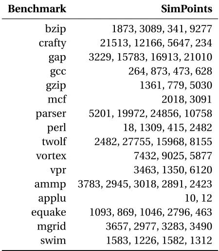
Table 3.3: SPEC SimPoints

Benchmark SimPoints

bzip 1873, 3089, 341, 9277 crafty 21513, 12166, 5647, 234 gap 3229, 15783, 16913, 21010 gcc 264, 873, 473, 628

gzip 1361, 779, 5030

mcf 2018, 3091

parser 5201, 19972, 24856, 10758 perl 18, 1309, 415, 2482 twolf 2482, 27755, 15968, 8155 vortex 7432, 9025, 5877

vpr 3463, 1350, 6120

ammp 3783, 2945, 3018, 2891, 2423

applu 10, 12

(47)

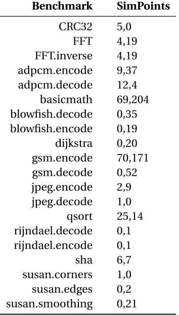
Table 3.4: MiBench SimPoints

Benchmark SimPoints

CRC32 5,0 FFT 4,19 FFT.inverse 4,19 adpcm.encode 9,37 adpcm.decode 12,4

basicmath 69,204 blowfish.decode 0,35 blowfish.encode 0,19 dijkstra 0,20 gsm.encode 70,171 gsm.decode 0,52 jpeg.encode 2,9 jpeg.decode 1,0

(48)

CHAPTER

4

Heterogeneous Multi-core Design

(49)

subsetting from G21 for robust performance is presented. Other workload-agnostic design approaches consisting of fewer cores are also presented and analyzed.

4.1

G21 - The Proposed Workload-agnostic Heterogeneous

Multi-core

Prior approaches of designing heterogeneous multi-cores for maximizing single thread per-formance relied on exhaustive evaluation of multi-core combinations[3]and time consuming design space explorations[12]. Further, these designs were tuned to a specific workload. It is uncertain how such designs would perform if the workload is changed. These drawbacks motivate a more robust approach of designing a heterogeneous multi-core.

Table 4.1: G21 widths and cycle times

superscalar width

2,3 4,5 6,7 8

cycle time (ns)

0.5 0.6 0.7 0.8 0.6 0.7 0.8 0.9 0.7 0.8 0.9 1.0

(50)

the cycle times and the width combinations. This results in a heterogeneous multi-core comprising of 21 core types, that provides ample microarchitectural diversity to capture the diverse nature of instruction-level parallelism (ILP). This 21-core heterogeneous multi-core

isgenericin nature because the constituent cores are chosen without any specific workload

in mind, hence the name G21.

(51)

Table 4.2: G21 cores

Core ID 0.5W2 0.6W2 0.7W2 0.5W3 0.6W3 0.7W3 0.6W4 0.7W4 0.8W4 0.6W5 0.7W5 0.8W5 0.7W6 0.8W6 0.9W6 0.7W7 0.8W7 0.9W7 0.8W8 0.9W8 1.0W8

Clock (ns) 0.5 0.6 0.7 0.5 0.6 0.7 0.6 0.7 0.8 0.6 0.7 0.8 0.7 0.8 0.9 0.7 0.8 0.9 0.8 0.9 1.0

I$ (KB) 16 64 128 16 64 128 64 128 128 64 128 128 128 128 128 128 128 128 128 128 128

D$ (KB) 16 64 128 16 64 128 64 128 128 64 128 64 32 64 64 32 64 64 64 64 64

L2$ (KB) 2048 2048 2048 2048 2048 2048 2048 2048 2048 2048 2048 2048 2048 2048 2048 2048 2048 2048 2048 2048 2048

Issue Q 32 48 64 16 48 64 32 48 64 24 48 64 32 48 64 24 48 48 24 48 48

LoadQ+StoreQ 96 128 128 96 128 128 128 128 128 128 128 128 128 128 128 128 128 128 128 128 128

Phy Reg File 128 192 512 64 128 512 128 384 512 64 192 384 128 256 512 64 192 512 128 384 512

Fetchwidth 2 2 2 3 3 3 4 4 4 5 5 5 6 6 6 7 7 7 8 8 8

Issue width 2 2 2 3 3 3 4 4 4 5 5 5 6 6 6 7 7 7 8 8 8

Fetch1 depth 3 3 3 3 3 3 3 3 3 3 3 3 3 3 3 3 3 3 3 3 2

Fetch2 depth 1 1 1 2 1 1 1 1 1 2 1 1 1 1 1 1 1 1 1 1 1

Decode depth 1 1 1 2 1 1 2 1 1 2 2 2 2 2 2 3 3 2 3 3 3

Rename depth 3 3 3 3 3 3 3 3 3 3 3 3 3 3 3 3 3 3 3 3 3

Issue loop depth 1 1 1 1 1 1 1 1 1 1 1 1 1 1 1 1 1 1 1 1 1

Issue depth 2 2 2 2 2 2 2 2 2 2 2 2 2 2 2 2 2 2 2 2 2

Reg Read depth 4 3 2 4 3 4 4 4 4 3 4 4 3 4 4 3 4 4 3 4 4

(52)

4.2

Performance Analysis of G21

In order to evaluate the performance robustness of G21, we obtain the maximum achievable performance (peak BIPS) for each benchmark by simulating it on every core in the design space. This exercise is performed simply to yield optimal yardsticks for comparison. Also, with exhaustive simulations, the overall best single core can be obtained. This core, referred to as Best-1, has the highest harmonic mean of BIPS over all benchmarks. Best-1 represents a homogeneous multi-core with only one core type. In all the results, ideal application to core steering is assumed. The performance for each application is expressed as a fraction of its highest achievable BIPS in the design space (peak BIPS).

0.0 0.1 0.2 0.3 0.4 0.5 0.6 0.7 0.8 0.9 1.0

bzip.1873 bzip.3089 bzip.341 bzip.9277

crafty.21513 crafty.12166 crafty.5647 crafty.234 gap.3229 gap.15783 gap.16913 gap.21010 gcc.264 gcc.873 gcc.473 gcc.628

gzip.1361 gzip.779 gzip.5030 mcf.2018 mcf.3091 parser.5201 _{parser.19972 parser.24856 parser.10758}

perl.18

perl.1309 perl.781 perl.415

twolf.2482 _{twolf.27755 twolf.15968} _{twolf.8155 vortex.7432 vortex.9025 vortex.5877} vpr.3463 vpr.1350 vpr.6120 _{ammp.3783 ammp.2945 ammp.3018 ammp.2891 ammp.2423} applu.10 applu.12

equake.1093 equake.869 equake.1046 equake.2796 equake.463 mgrid.3657 mgrid.2977 mgrid.3283 mgrid.3490 swim.1583 swim.1226 swim.1582 swim.1312

AVERAGE

BIPS

/

peak

BIPS

Best‐1

G21

(53)

Figure 4.1 shows the performance of G21. G21 achieves97 percentof peak achievable per-formance, despite the fact that it was not trained or designed for any specific workload. This demonstrates the performance robustness of G21. Further, no benchmark degrades more

than12 percentfrom its peak. This is especially remarkable when compared to Best-1, which

suffers up to 30 percent degradation for

bzip.341

. Although, Best-1 delivers reasonably good performance overall (within 11% of peak), several benchmarks suffer heavy degradation. Since Best-1 was trained (chosen specifically) for the workload of the 59 benchmarks, it is likely that it may degrade even more for unseen workloads. The robustness of G21 on 59 benchmarks highlights the merit of workload-agnostic design and provides confidence that it will be able to deliver high performance even for unseen workloads.

(54)

0.000

0.250

0.500

0.750

1.000

1.250

1.500

1.750

2.000

2.250

bzip.2602 bzip.6110 bzip.8219 bzip.9148 bzip.4928

crafty.12427 crafty.8225 crafty.8058 crafty.3947 crafty.20426 gap.15090

gap.5051 _{gap.16939 gap.21307 gap.13096} gcc.658 gcc.621 gcc.20 _{gcc.371 gcc.544}

gzip.5276

gzip.0

gzip.1042 gzip.2743 gzip.265 mcf.2001 mcf.3668 mcf.1677 mcf.3431 mcf.1197 parser.27403 parser.28805 parser.6740 parser.10107 parser.17444

perl.1996 per

l.90

perl.3300 perl.2977 perl.2221

twolf.28139 twolf.23611 twolf.15150 twolf.2817 twolf.7051 vortex.7794 vortex.374 vortex.18 vortex.7124 vortex.5064 vpr.3638 vpr.1089 vpr.3045 vpr.9446 vpr.3432

ammp.3205 ammp.168 ammp.2250 ammp.1544 ammp.4410 applu.8 _applu.48 applu.0 _applu.36 applu.7

apsi.73137 apsi.17531 apsi.73359 apsi.74172 apsi.65683 equake.451 _equake.2095 equake.336 _equake.1992 equake.33 mgrid.3044 mgrid.1833 mgrid.1639 mgrid.3502 mgrid.3258 swim.464 swim.477 swim.769 swim.585 swim.693

HMEAN

Speed

up

(55)

G21 performs almost 20% better than Best-1, on average. Since Best-1 was trained for a different workload, it shows significant performance disadvantage compared to G21. Further, for several benchmarks from the new workload, G21 significantly outperforms Best-1: up to 211% for

swim.585

. This highlights the vulnerability of the training cores to workloads. The new workload happen to include several SimPoints, mainly from floating-point benchmarks, that prefer large window cores. Further, SimPoints from

applu

benefitted from both, a large window and a larger issue width. Best-1 does not have a large window to accommodate these new SimPoints and consequently performs poorly on them. Obtaining the optimal performance for the 85 benchmarks requires several months of compute time to perform design space explorations. The robustness of G21 on the previous workload provides some confidence that G21 would deliver near optimal performance even for the new workload.

4.3

Other Workload-agnostic Design Approaches

(56)

performance for a large number of benchmarks.

This dissertation also explores approaches for achieving robust performance using fewer of cores, based on known microarchitectural insights. Three approaches for a robust workload-agnostic heterogeneous multi-core design are discussed the following sections. The multi-cores designed using these approaches are evaluated on the integer benchmarks from the SPEC CPU 2000 suite. From the previous 59 SimPoints, the 41 SimPoints correspond-ing to the integer benchmarks are used as the workload. A comparison with the previous Best-1 is made to show the robustness of these approaches.

4.3.1

Approach 1: Square-root Law

(57)

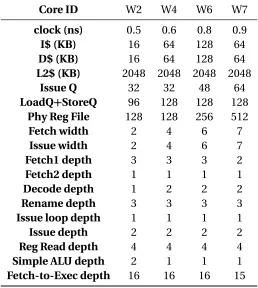
Table 4.3: Cores of SQL-4

Core ID W2 W4 W6 W7

clock (ns) 0.5 0.6 0.8 0.9

I$ (KB) 16 64 128 64

D$ (KB) 16 64 128 64

L2$ (KB) 2048 2048 2048 2048

Issue Q 32 32 48 64

LoadQ+StoreQ 96 128 128 128

Phy Reg File 128 128 256 512

Fetch width 2 4 6 7

Issue width 2 4 6 7

Fetch1 depth 3 3 3 2

Decode depth 1 2 2 2

Rename depth 3 3 3 3

Issue loop depth 1 1 1 1

Issue depth 2 2 2 2

Reg Read depth 4 4 4 4

Simple ALU depth 2 1 1 1

(58)

Figure 4.3 shows the performance of the 4-core heterogeneous multi-core based on the square-root law (referred to as SQL-4) and Best-1. SQL-4 achieves 95% of peak achievable performance. Further, it almost always performs better than Best-1. A couple of benchmarks

bzip.341

and

gcc.264

experience degradations of 19% and 21% respectively from the peak

performance in the design space. The same benchmarks, suffer close to 30% degradation on Best-1. Several other benchmarks also suffer significant degradations on Best-1, but SQL-4 is able to limit them reasonably.

0.0 0.2 0.4 0.6 0.8 1.0

bzip.1873 bzip.3089 bzip.341 bzip.9277

crafty.21513 crafty.12166 crafty.5647 crafty.234

gap.3229 _gap.15783 _gap.16913 _gap.21010 gcc.264 gcc.873 gcc.473 gcc.628 gzip.1361 gzip.779 gzip.5030 mcf.2018 mcf.3091

parser.5201 _parser.19972 _parser.24856 _parser.10758

perl.18

perl.1309 perl.781 perl.415 _twolf.2482

twolf.27755 twolf.15968 twolf.8155 vortex.7432 vortex.9025 vortex.5877

vpr.3463 vpr.1350 vpr.6120 _AVERAGE

BIPS

/

Peak

BIPS

Best‐1 SQL‐4

(59)

4.3.2

Approach 2: Near and Far ILP

Some applications are serial in nature. The code of such applications is generally character-ized by few long serial dependence chains. To extract ILP from such applications, a larger window is necessary to look further down the instruction stream for independent instruc-tions. Such applications do not require a large issue width (due to low available of ILP) but require a large instruction window.

On the other hand, some applications have many short dependence chains providing many independent instructions in close proximity. For example, dynamic unrolling of a short loop with few loop-carried dependences results in significant extractable ILP. Such application with plenty of "near" ILP do not require a large instruction window (due to the free-flowing nature of instructions) but they benefit from a large issue width.

(60)

Table 4.4: Cores of FNILP-7

Core ID W2 W4N W6N W8N W4F W6F W7F

clock (ns) 0.5 0.5 0.7 0.8 0.8 1 1.2

I$ (KB) 16 32 128 128 128 128 128

D$ (KB) 16 64 128 128 128 64 64

L2$ (KB) 2048 2048 2048 2048 2048 2048 2048

Issue Q 32 16 24 48 64 96 128

LoadQ+StoreQ 96 64 64 64 128 128 128

Phy Reg File 128 64 128 128 512 512 512

Fetch width 2 4 6 8 4 6 7

Issue width 2 4 6 8 4 6 7

Fetch1 depth 3 3 3 3 3 2 2

Fetch2 depth 1 2 1 1 1 1 1

Decode depth 1 2 2 3 1 1 1

Rename depth 3 3 3 3 3 2 2

Issue loop depth 1 1 1 1 1 1 1

Issue depth 2 2 2 2 2 2 2

Reg Read depth 4 4 3 3 4 3 3

Simple ALU depth 2 2 1 1 1 1 1

(61)

Figure 4.4 shows the performance of the 7-core heterogeneous multi-core with cores for extracting far and near ILP (referred to as FNILP-7). FNILP-7 achieves 95% of peak perfor-mance. The only benchmark that significantly degrades is

gcc.264

, showing a degradation of 17%. Most other benchmarks achieve at least close to 90% of their peak performance. The ability of FNILP-7 in capturing significant ILP diversity demonstrates its robustness.

0.0 0.2 0.4 0.6 0.8 1.0

bzip.1873 bzip.3089 bzip.341 bzip.9277

perl.18

perl.1309 perl.781 perl.415

twolf.2482 _twolf.27755 _twolf.15968 twolf.8155 _vortex.7432 _vortex.9025 _vortex.5877 vpr.3463 vpr.1350 vpr.6120 AVERAGE

BIPS

/

Peak

BIPS

Best‐1 FNILP‐7

Figure 4.4: Performance of FNILP-7. Performance is normalized to peak achievable perfor-mance in the entire design space.

4.3.3

Approach 3: Iso-frequency Approach

(62)

cores need to access shared resources such as the last level cache and the interconnection network. With the cores running at different frequencies, additional hardware becomes necessary to manage interactions with shared resources, even if only one core is active at a time (single-thread execution).

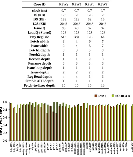
The Iso-frequency approach can mitigate this difficulty by restricting the choice of cores to single frequency domain. In this approach, a clock frequency and 4 cores with issue widths of 2, 4, 6 and 8 are chosen. After initial experiments, multi-cores with lower frequency were found to be severely sub-optimal. The clock frequency corresponding to the clock period of 0.7ns was found to be competitive. For the cycle time of 0.7ns, 4 cores with superscalar widths of 2, 4, 6 and 7 are chosen. The cycle time of 0.7ns does not accommodate any core design with width of 8, hence the issue width of 7 was selected instead. For the given combination of frequency and issue width, pipeline depth was maximized. Table 4.5 shows the configurations of the core designs.

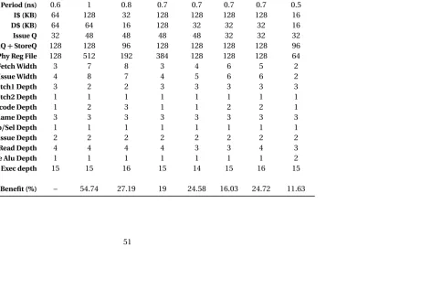
Figure 4.5 shows the performance of the 4-core heterogeneous multi-core with all cores with a cycle time of 0.7ns (referred to as ISQFREQ-4). ISQFREQ-4 achieves over 93% of peak perfomance overall. The maximum degradation that any benchmark experiences is 15%.

4.4

Subsetting from G21

(63)

Table 4.5: Cores of ISOFREQ-4

Core ID 0.7W2 0.7W4 0.7W6 0.7W7

clock (ns) 0.7 0.7 0.7 0.7

I$ (KB) 128 128 128 128

D$ (KB) 128 128 32 16

L2$ (KB) 2048 2048 2048 2048

Issue Q 96 48 32 32

LoadQ+StoreQ 128 128 128 128

Phy Reg File 512 384 128 64

Fetch width 2 4 6 7

Issue width 2 4 6 7

Decode depth 1 1 2 3

Rename depth 3 3 3 3

Issue loop depth 1 1 1 1

Issue depth 2 2 2 2

Reg Read depth 4 4 3 3

Simple ALU depth 1 1 1 1

Fetch-to-Exec depth 15 15 15 16

0.0 0.2 0.4 0.6 0.8 1.0

bzip.1873 bzip.3089 bzip.341 bzip.9277

perl.18

perl.1309 perl.781 perl.415 _twolf.2482

twolf.27755 twolf.15968 twolf.8155 vortex.7432 vortex.9025 vortex.5877

vpr.3463 vpr.1350 vpr.6120 _AVERAGE

BIPS

/

Peak

BIPS

Best‐1 ISOFREQ‐4

(64)

highly representative of the design space. If the workload is known a priori, fewer cores from G21 can be chosen for single-thread performance to capture the known ILP diversity. Two approaches to distilling the cores are explored.

Best-N-of-G21: These are N cores from G21 that provide the highest harmonic mean BIPS over all the benchmarks.

Robust-N-of-G21: These are N cores from G21 that minimize the peak degradation for any benchmark.

Table 4.6: G21 subsetting strategies

N Best-N-of_G21 Robust-N-of-G21

Relative Perf. Max % degradation Relative Perf. Max % degradation

1 0.924 27.1 0.924 27.1

2 0.965 19.3 0.951 13.7

3 0.977 15.4 0.967 13.5

4 0.985 15.4 0.976 10.6

5 0.992 11.0 0.98 9.7

6 0.996 5.1 0.996 5.1

7 0.998 3.9 0.998 3.9

8 0.998 3.9 0.998 3.9

(65)

benchmark’s peak performance on G21. The results demonstrate a trade-off between achiev-ing the highest possible performance and boundachiev-ing the peak degradation for any benchmark. For instance, Robust-3-of-G21 achieves the same performance as Best-2-of-G21 but limits the maximum degradation to 13.5% as compared to 19.3% for Best-2-of-G21. The Best-2-of-G21 comprises of the cores

0.6W4

and

0.8W5

. The core

0.6W4

achieves high performance for most of integer benchmarks, whereas

0.8W5

covers most of the floating-point benchmarks. Although, Best-2-of-G21 delivers high overall performance, benchmarks such as

bzip.3089

perform 19.3% worse than their peak on G21. Robust-3-of-G21 comprises of

0.7W3

,

0.7W6

and

0.9W7

. At the cost of an extra core, Robust-3-of-G21 is better able to capture these outlier

benchmarks. Typically, these benchmarks perform well on very few cores in G21. The bench-mark that suffers the greatest degradation on Robust-3-of-G21 is

mcf.3091

, which being a memory-bound serial benchmark, prefers a narrow and high frequency core. A similar relation is also observed in case of Robust-4-of-G21 and Best-3-of-G21. The Robust-N-of-G21 strategy sacrifices average performance by choosing cores that capture outlier benchmarks.

4.5

Understanding Application Characteristics and Preferred

Architectural Configurations

(66)

individual phase performance, we find the highest performing core in the design space, i.e.

thecustomized core, for SimPoints from SPEC Integer benchmarks. We also obtain the core

(67)

Table 4.7: The best homogeneous core and customized cores of theoutlierSimPoints

Best-1 bzip.3089 bzip.341 gap.3229 gcc.264 gcc.473 gcc.628 mcf.2018

Clock Period (ns) 0.6 1 0.8 0.7 0.7 0.7 0.7 0.5

I$ (KB) 64 128 32 128 128 128 128 16

D$ (KB) 64 64 16 128 32 32 32 16

Issue Q 32 48 48 48 48 32 32 32

LoadQ+StoreQ 128 128 96 128 128 128 128 96

Phy Reg File 128 512 192 384 128 128 128 64

Fetch Width 3 7 8 3 4 6 5 2

Issue Width 4 8 7 4 5 6 6 2

Fetch1 Depth 3 2 2 3 3 3 3 3

Fetch2 Depth 1 1 1 1 1 1 1 1

Decode Depth 1 2 3 1 1 2 2 1

Rename Depth 3 3 3 3 3 3 3 3

Wakeup/Sel Depth 1 1 1 1 1 1 1 1

Total Issue Depth 2 2 2 2 2 2 2 2

Reg Read Depth 4 4 4 4 3 3 4 3

Simple Alu Depth 1 1 1 1 1 1 1 2

Fetch to Exec depth 15 15 16 15 14 15 16 15

(68)

To understand why these SimPoints perform significantly better on their customized core, it is important to understand their characteristics. Studying them at the source-code and assembly-code level lends insight into how these characteristics relate to the SimPoint’s customized core in the design space. For conciseness, the following sections analyze the code of 4 of the 7 SimPoints. The same approach can be extended to any other SimPoint.

4.5.1

Case Study I:

gap.3229

This SimPoint performs 19% better on its customized core than on the best homogeneous design. A single basic block of 4 instructions accounts for over 85% for its execution. The C source code of the bencmark is shown in Figure 4.6.

s = d+1;

e = PTR(HdFree);

while ( s < e )

*s++ = 0;

Figure 4.6: C code from

gap.3229

(69)

This loop exhibits a high data cache miss rate indicating that it iterates over a large address range which cannot be accommodated in the cache memory. Such a loop can be accelerated if the memory accesses are served in parallel, suggesting ample opportunity to exploit memory-level parallelism (MLP). A core with a large instruction window is more suitable in this case since later independent instructions can be buffered and executed which older memory accesses are being serviced. Apart from the customized core, other top performing cores for

gap.3229

also indicate a strong preference for a large instruction window.

4.5.2

Case Study II:

mcf.2018

while( arcin ) {

tail = arcin->tail;

if(tail->time + arcin->org_cost > latest) {

arcin = (arc_t *)tail->mark;

continue; }

red_cost = arc_cost - tail->potential + head_potential;

… …

arcin = (arc_t *)tail->mark;

}

mcf.2018

(70)

from the function

price_out_impl

in

implicit.c

which dominates the execution of the benchmark. Some fragments of code such as the not-taken path of a branch that is usually taken are indicated by . . . as they not important for any analysis. Each iteration depends on the data (next address) loaded in the previous iteration. Also, the next address deferences cause high data cache miss rate and serialize the chain of computation. The frequent occurrence of a branch instruction also limits fetch bandwidth. Such a serial benchmark benefits more on a narrow core with smaller structures and a high clock frequency.

4.5.3

Case Study III:

bzip.3089

Figure 4.8 shows the code fragment from the function

sortIt

in

bzip2.c

. This code frag-ment exhibits ample potential instruction-level parallelism. However, the presence of a load with irregular address computation and an indirect store (as highlighted) causes a larger number of data cache misses. But more importantly, there are no major loop carried de-pendences (except one) which makes this loop easily software pipelinable. A larger register window allows dynamic unrolling of the loop and the data cache misses can be overlapped.

bzip.3089

performs best on a wide-issue core since there is plenty of ILP available. The

(71)

for (i = 0; i < last; i++) {

c2 = block[i+1]; j = (c1 << 8) + c2; c1 = c2;

ftab[j]--;

zptr[ftab[j]] = i;

}

bzip.3089

for (offset=0, i=0; offset < regset_size; offset++)

for (bit = 1; bit; bit <<= 1, i++) { if (i == max_regno)

… …

if (old[offset] & bit) { … …

} } }

(72)

4.5.4

Case Study IV:

gcc.473

Figure 4.9 shows the code fragment from the function

propagate_block

in

flow.c

. This code fragment accounts for over 50% of the benchmark’s execution. This code fragment

of

gcc.473

has very few data cache misses and the branches are highly predictable. Most

of the computation within an iteration of the inner loop is independent. Also, bec

Architecting a Workload-agnostic Heterogeneous Multi-core Processor.

ABSTRACT

APPROVED BY:

DEDICATION

TABLE OF CONTENTS

LIST OF TABLES . . . x

Chapter 4 Heterogeneous Multi-core Design. . . 32

Chapter 5 ILP Characterization and Workload-agnostic Core Selection. . . 60

Chapter 6 Application Steering . . . 93

LIST OF TABLES

LIST OF FIGURES

CHAPTER

Contributions

Outline

CHAPTER

Statistical Simulation

Design Space

Realistic Pruning of the Design Space

Canonical Interfaces

Modeling of Clocked Structures

stall

Simulator Optimizations and Features

FabSim

Validation of FabSim

Core-1 Core-2 Core-3 Core-4 Core-5 Core-6 Core-7 Core-8 Core-9 Core-10

wakeup-select loop

Performance trend - bzip

Verilog C++

Benchmarks

Benchmark SimPoints

CHAPTER

superscalar width

Core ID 0.5W2 0.6W2 0.7W2 0.5W3 0.6W3 0.7W3 0.6W4 0.7W4 0.8W4 0.6W5 0.7W5 0.8W5 0.7W6 0.8W6 0.9W6 0.7W7 0.8W7 0.9W7 0.8W8 0.9W8 1.0W8

Performance Analysis of G21

bzip.1873 bzip.3089 bzip.341 bzip.9277

AVERAGE

bzip.2602 bzip.6110 bzip.8219 bzip.9148 bzip.4928

HMEAN

Approach 1: Square-root Law

bzip.1873 bzip.3089 bzip.341 bzip.9277

Approach 2: Near and Far ILP

bzip.1873 bzip.3089 bzip.341 bzip.9277

Approach 3: Iso-frequency Approach

Subsetting from G21

bzip.1873 bzip.3089 bzip.341 bzip.9277

N Best-N-of_G21 Robust-N-of-G21

Understanding Application Characteristics and Preferred

Case Study I:

Case Study II:

while( arcin ) {

price_out_impl

for (i = 0; i < last; i++) {

Case Study IV: