Approaches for Graphs Near Structural Classes.

(1)

ABSTRACT

VAN DER POEL, ANDREW JOHN. Approaches for Graphs Near Structural Classes. (Under the direction of Blair D. Sullivan.)

Many real-world networks arise from processes which imply that the graph should have a particular structure. Unfortunately, often noise and errors in the data prevent this structure from existing, confounding, and in some cases, preventing analysis. One approach to resolving this discrepancy is through graph modification – the addition and deletion of nodes and edges until the resulting graph has some desired property. Modification problems are well-studied in graph theory, and are of particular interest to algorithm designers for graphs which are close to a structural class, since they naturally lend themselves to parameterization. Recently, they have also been used in the structural rounding technique of Demaine et al. for extending approximation algorithms.

Historically, most work on graph modification has focused on finding a (smallest) set of edits, but algorithmically it can also be interesting to use structure implied by an edit set to solve other classically hard problems. These settings naturally lend themselves to both exact and approximate variants of problems.

This dissertation focuses on expanding the frontier of graph modification algorithms, and does so in several directions, mixing approximation and parameterization. First, we give an exact algorithm for the parameterized version of the problem of finding an edge edit set whose deletion yields a path forest, significantly reducing the best-known complexity. We also give two novel algorithms which exactly enumerate all maximal induced complete bipartite subgraphs for graphs which are near-bipartite (have a small vertex edit set to some near-bipartite graph) and provide an empirical comparison with the state-of-the-art approach on general graphs. Finally, we develop a suite of algorithms for "lifting" solutions to Vertex Cover within the structural rounding framework (extending solutions on a subgraph to apply to the entire graph). We experimentally evaluate the effectiveness of these approaches on both synthetic and real-world graphs.

(2)

(3)

Approaches for Graphs Near Structural Classes

by

Andrew John van der Poel

A dissertation submitted to the Graduate Faculty of North Carolina State University

in partial fulfillment of the requirements for the Degree of

Doctor of Philosophy

Computer Science

Raleigh, North Carolina

2019

APPROVED BY:

Steffen Heber Carla D. Savage

Matthias F. Stallmann Blair D. Sullivan

(4)

DEDICATION

(5)

BIOGRAPHY

(6)

ACKNOWLEDGEMENTS

I would like to thank Dr. Blair D. Sullivan for her years of advising and assistance with shaping this work. I deeply appreciate the opportunity I was given in her lab and the patience and respect I was always shown. Many thanks to Dr. Felix Reidl and Dr. Kyle Kloster for their guidance within the lab and, more importantly, their friendship outside. Likewise, my fellow PhD students Dr. Michael P. O’Brien, Timothy D. Goodrich, Brian Lavallee, and Michael Breen-McKay were always willing to lend a helping hand and work through problems together, while being the source of many laughs. You have all made my time as PhD student incredibly rewarding and enjoyable.

Thank you to my committee members, Dr. Steffen Heber, Dr. Carla D. Savage, and Dr. Matthias F. Stallmann, for your insights, feedback, and questions regarding this dissertation. It is an honor to have such talented faculty as part of my committee. I would also like to thank faculty members from Saint Rose, Dr. Jim Teresco, Dr. Amina Eladdadi, and Dr. Mary Ann McLoughlin for encouraging me to pursue this degree and serving as great ambassadors for higher education.

(7)

copath

. . . 20

3.5 Conclusion . . . 21

Chapter 4 MINING MAXIMAL INDUCED BICLIQUES USING ODD CYCLE TRANSVERSALS 22 4.1 Introduction . . . 23

4.2.1 Related work . . . 24

4.2.2 Notation and Terminology . . . 25

4.3

OCT-MIB

. . . 26

4.3.1 Algorithm outline & data structure . . . 27

4.3.2 Algorithm Details . . . 29

4.3.3

MCB

Algorithm . . . 31

4.3.4 Correctness & Complexity:

OCT-MIB

. . . 32

4.3.5 Correctness & Complexity:

MCB

. . . 33

4.4

OCT-MIB-II

. . . 34

4.4.1 Algorithm Framework . . . 34

4.4.2

Enum-MIB

. . . 36

4.4.3

OCT-MIB-II

. . . 36

4.4.4 Algorithm Subroutines . . . 37

(8)

4.5 Implementation Details . . . 39

4.6 Empirical Evaluation . . . 40

4.6.1 Data and experimental setup . . . 40

4.6.2 Initial Benchmarking . . . 41

4.6.3 Larger Graphs . . . 42

4.6.4 Computational Biology Data . . . 46

4.7 Discussion of Dias et al. . . 48

4.7.1 Modified

Dias

. . . 50

4.8 Extremal Case for Zhang et al. . . 51

4.9 Conclusions . . . 52

Chapter 5 APPROXIMATING VERTEX COVER USING STRUCTURAL ROUNDING. . . 53

5.1 Introduction . . . 53

5.2.1 Structural Rounding . . . 54

5.2.2 VERTEXCOVER2-Approximations . . . 56

5.2.3 Odd Cycle Transversals . . . 56

5.3 Lifting Algorithms . . . 56

5.3.1 Naïve Lifting . . . 57

5.3.2 Greedy Lifting . . . 57

5.3.3 2-Approximation Lifting . . . 57

5.3.4

oct-first

Lifting . . . 58

5.3.5

bip-first

Lifting . . . 58

5.3.6 Recursive Lifting . . . 59

5.4 Experimental Setup . . . 59

5.4.1 Synthetic Data . . . 59

5.4.2 Real World Data . . . 60

5.4.3 Measuring Quality . . . 60

5.4.4 Hardware . . . 61

5.5 Implementation . . . 61

5.5.1 2-Approximation Variants . . . 63

5.5.2 Finding OCT Sets . . . 63

5.5.3 Converting Maximum Matchings . . . 63

5.5.4 Variance Between Runs . . . 64

5.6 Experimental Evaluation . . . 64

5.6.1 Impact of Generator Parameters . . . 66

5.6.2 Procured Results . . . 68

5.6.3 Real-world Experiments . . . 71

5.7 Conclusion . . . 73

Chapter 6 CONCLUSION & FUTURE WORK . . . 74

(9)

LIST OF TABLES

Table 3.1 Dynamic programming table parameters and upper bounds. . . 15 Table 3.2 Numerically obtained constantscd, 3≤d≤17, used in Lemma 4; originally

given in Table 6.1 of[Gas10]. . . 19

Table 4.1 The runtimes (rounded to nearest thousandth-of-a-second) of the biclique-enumeration algorithms on the Afro-American subset of the Wernicke-Hüffner computational biology data[Wer14]. . . 49 Table 4.2 The runtimes (rounded to nearest thousandth-of-a-second) of the

biclique-enumeration algorithms on the Japanese subset of the Wernicke-Hüffner computational biology data[Wer14]. . . 50

Table 5.1 Summary statistics of real-world corpus. . . 60 Table 5.2 Mean solution sizes for and standard deviations of 2-approximation

vari-ants on the 100K corpus. We employ three edge selection techniques for

standard

: incident to a high-degree vertex (

std-high

), incident to a low-degree vertex (

std-low

), and arbitrarily (

std-rand

). We note that the large standard deviations are due to the relatively high variety of graphs in the corpus. . . 61 Table 5.3 We ran our framework 50 times on each graph in our corpus with 100K

(10)

LIST OF FIGURES

Figure 3.1 Three co-path sets (dashed edges), including one of minimum size (rightmost). 8

Figure 4.1 An example of a biclique which is not induced (blue edges), an induced biclique which is not maximal (red edges), and a maximal induced biclique (green edges). The blue edges do not form an induced biclique because vertices 2 and 3 share an edge. The red edges do not form a maximal biclique because vertex 8 is independent from vertex 7 and shares edges with vertices 4 and 5. . . 25 Figure 4.2 Ifvis the vertex we initialize with, our initial bicliques will be{v}×{x,z}and

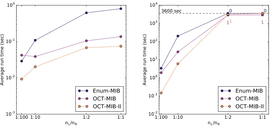
{v} × {y,z}, noting thatx andy cannot be on the same side of an induced biclique because they share an edge. When we expand these initial bicliques withw, the expanded bicliques are{v,w} × {x,z}and{v,w} × {z}, with the latter being subsumed by the former. . . 27 Figure 4.3 Runtimes of

OCT-MIB

and

LexMIB

under varied bipartite balance conditions.

FornB=200 (Left, andnB=1000 (Right), each curve represents the runtime in seconds of an algorithm on graphs with a given OCT size and varied balance. WhennBwas 1000,

OCT-MIB

timed out (3600s) on 90% of instances with balance 1:1 and 1:2.

LexMIB

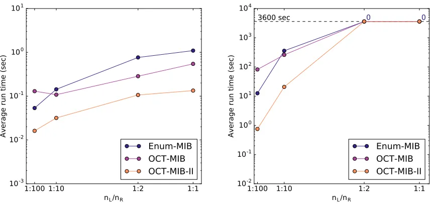
timed out on 100% of instances at these settings, as well as 70% of those with balance 1:10. . . 40 Figure 4.4 Runtimes of the MIB-enumerating algorithms on graphs wherenB=1000,

nL/nR =10, and the expected edge density betweenOandL∪Rwas varied with all other densities were 0.05.n_O =10 in the left panel andn_O =3 log₃n_B in the right panel. . . 41 Figure 4.5 Runtimes of the MIB-enumerating algorithms on graphs wherenO =10 and

the ration_L/n_R was varied. The left panel hasn_B=200 and the right panel hasnB =1000. . . 42 Figure 4.6 Runtimes of the MIB-enumerating algorithms on graphs wherenO =19≈

3 log₃(n_B)and the ration_L/n_R was varied. The left panel hasn_B=200 and the right panel hasnB=1000. . . 43 Figure 4.7 Runtimes of the MIB-enumerating algorithms on graphs wherenO =10 and

the coefficient of variation betweenLandRwas varied. The left panel has nB=200 and the right panel hasnB=1000. . . 43 Figure 4.8 Runtimes of the MIB-enumerating algorithms on graphs wherenO =19≈

3 log₃(nB)and the coefficient of variation betweenLandRwas varied. The left panel hasnB=200 and the right panel hasnB=1000. . . 44 Figure 4.9 Runtimes of the MIB-enumerating algorithms on graphs wherenB=1000

andnO was varied. . . 44 Figure 4.10 Runtimes of the MIB-enumerating algorithms on graphs wherenB=1000

and the expected edge density withinOwas varied. The left panel hasnO= 10 and the right panel hasnO ==19≈3 log3(nB). . . 45 Figure 4.11 Runtimes of the MIB-enumerating algorithms on graphs wherenB =150,

(11)

Figure 4.12 Runtimes of the MIB-enumerating algorithms on graphs wherenB =200, nL =nR andnO =5. The expected edge density between L and R and between{L,R}andOwas varied. In the left panel the expected edge density withinOwas fixed to 0.05 and in the right panel it varied with the rest of the graph. . . 46 Figure 4.13 Runtimes of the MIB-enumerating algorithms on graphs wherenB =300,

nL =nR andnO =5. The expected edge density between L and R and between{L,R}andOwas varied. In the left panel the expected edge density withinOwas fixed to 0.05 and in the right panel it varied with the rest of the graph. . . 46 Figure 4.14 Runtimes of the OCT-based MIB-enumeration algorithms on graphs where

n_B=10000 andn_Ovaries. In the left panel,n_L=9901,n_R=99 (n_L/n_R≈100) and the expected edge density is 0.03. In the right panel,nL=9091,nR=909 (nL/nR≈10) and the expected edge density (excluding withinO) is 0.01; the marker-type denotes the expected edge density withinO(see legend). For these larger instances we used 3 seeds and a 7200s timeout. . . 47 Figure 4.15 Runtimes of the MIB-enumerating algorithms on graphs wherenL/nR =9

and all expected edge densities are 0.05.n_B is varied (x-axis) and the marker-type denotes the value ofnO ∈ {10,pnB, 3 log3(nB)}(see legend). The time-out value is set to 7200s. . . 47 Figure 4.16 An example of a graph where

Dias

would not find all MIBs. The MIBC =

{1, 3} × {5}would not be found. In the notation of the algorithm j=3 and B={0, 1, 4} × {2}should yieldC. WhenXj ={0, 1}, no biclique is found as

{0, 1, 3}have no common neighbors. WhenX_j={2}the biclique{2, 3}×{4}is found. Even if we removed the if-condition on line 12, whenj=5 we would add the bicliques{1, 4} × {5}and{0, 5} × {2}toQ. WhenB={0, 5} × {2}(line 7), no new bicliques are added toQand then the next least biclique output in line 6 would not beC. . . 51 Figure 4.17 An example of a graph in which

iMBEA

would run in timeΩ(B m n). . . 52

Figure 5.1 An example of structural rounding when vertex deleting to bipartite graphs while solving VERTEXCOVER. The red vertices are the edit setD, the blue vertices the partial solutionS0, and the green vertices,I0, are the ones not added to the partial cover. Note thatS0_{is an optimal vertex cover on}_G_[_S0_∪_I0_]_,

which is bipartite. . . 57 Figure 5.2 Mean relative OCT sizes for OCT decomposition algorithms on the 100K

corpus, partitioned by prescribed OCT ratio. Approaches include a BFS-based technique (bfs), and the construction of two maximal independent sets with three vertex selection rules: arbitrarily (random), by minimum initial degree (no re-sort), and by minimum degree with re-sorting (re-sort). 61 Figure 5.3 Distribution of procured OCT sizes relative to prescribed OCT sizes found

(12)

Figure 5.4 Average approximation ratios (left) and relative runtime (right) on the full synthetic corpus, partitioned by expected number of edges. For 4M edge graphs, we use both procured (“pro") and prescribed (“pre") OCT decom-positions. Runtimes are given relative to that of

standard

, which is fastest on average (mean runtimes: 1.511s on 4M-pro, 1.502s on 4M-pre, 20.551s on 40M, and 136.779s on 200M). For structural rounding approaches, the time it takes to find the OCT decompositionisaccounted for in the runtime (note that for 4M-pre, this contributes zero since the decomposition is given as input). . . 62 Figure 5.5 Two settings when more sophisticated lifting strategies outperform

naïve

and

greedy

on the 4M-pro data. We partition graphs based on two generator parameters: relative OCT set size (top), and expected edge density withinO (bottom). . . 65 Figure 5.6 The average approximation ratios over all synthetic graphs with 4-million

expected edges in the prescribed setting, with 4-million expected edges in the procured, with 40-million expected edges, and with 200-million expected edges separated by|L|/|R|. . . 67 Figure 5.7 The average approximation ratios over all synthetic graphs with 4-million

expected edges in the prescribed setting, with 4-million expected edges in the procured, with 40-million expected edges, and with 200-million expected edges separated by the expectedc v betweenOand{L,R}. . . 68 Figure 5.8 The average approximation ratios over all synthetic graphs with 4-million

expected edges in the prescribed setting, with 4-million expected edges in the procured, with 40-million expected edges, and with 200-million expected edges separated by the proportion of the graph which is inO. . . 69 Figure 5.9 The average approximation ratios over all synthetic graphs with 4-million

expected edges in the prescribed setting, with 4-million expected edges in the procured, with 40-million expected edges, and with 200-million expected edges separated by the expected edge density withinO. . . 70 Figure 5.10 The average approximation ratios over all synthetic graphs with 4-million

expected edges in the prescribed setting and in the procured separated by the expected edge density betweenOand{L,R}. . . 71 Figure 5.11 The mean approximation ratios over all synthetic graphs with 4-million

ex-pected edges in the prescribed setting and in the procured setting, separated by the expected edge density betweenLandR. . . 71 Figure 5.12 Correspondence between the size of the procured OCT set and solution

(13)

(14)

CHAPTER

1

INTRODUCTION

1.1

Motivation

Data from a wide array of fields can be modeled as interactions in a network. Viewing data through this lens has naturally led to network analysis and graph algorithms being extremely useful tools in many different domains. Unfortunately, many graph problems are computationally difficult to solve. However, when networks have specific structure, they are much easier to work with, and common tasks may become much faster when restricted to particular classes of graphs. In the real-world, data simply does not have the structure which is necessary to take advantage of the aforementioned structure-based algorithms. Quite often this can be attributed to noise and errors within the data, which prevent the domain networks from belonging to any rigid class.

(15)

structure).

Designing new efficient graph modificiation algorithms for graphs near structural classes is the main idea of this dissertation. We work with structural classes as opposed to spectral or other types of graph classes because they naturally capture desired features of real-world data. Editing algorithms perform best on graphs near structural classes, as opposed to ones which are not “close" to having structure, because the number of modifications is small. Further, advances in this space apply to a much larger set of graphs than when working with the more rigid, traditional classes. We consider three types of graph modification problems in a naturally advancing progression. The first exploits being close to a structural class to find an edit set via a parameterized algorithm. This is similar to the zoological example mentioned above, and is in many ways the “traditional” type of modification problem. Second, we consider the case where we are given an edit set, rather than being tasked with finding one. In this setting we leverage the structure implied by a small edit set to exactly solve a problem on the entire graph (both the edit set and the rest of the graph). We further extend this idea to approximately solving problems on the entire graph. Rather than solving a problem exactly, approximation algorithms give theoretical guarantees on the size of a solution it produces relative to the optimal solution.

Our work demonstrates that designing exact and approximation algorithms which both find edit sets and take advantage of the structure implied by edit sets are relevant, realistic, and robust approaches for utilizing graph-based techniques to solve real-world problems.

1.2

Research Directions and Outline

This work expands the algorithmic frontier of graph modification in a number of ways. We made progress in each direction by focusing on specific problems, which I now describe, along with an outline of how the document proceeds. Chapter 2 describes the necessary background on graph theory, computational complexity, and algorithmic methods to understand the research. In Chapter 3, we solve a parameterized problem where we want to find an edit set. Namely, thek-CO-PATHSET problem asks if there exists a set ofk edges whose removal yields a network where all connected components are paths? We solve this problem by giving a novel, fastest-known algorithm, which utilizes kernelization, branching, and the Cut & Count technique.

We then work on a second parameterized problem, but in the setting where we are given an edit set and aim to leverage the implied structure. In Chapter 4, we are given a graph with a set of nodes whose removal leaves a bipartite graph and describe two novel algorithms which enumerate all maximal induced complete bipartite subgraphs in such a graph. We also provide an open-source implementation and experimentally evaluate our approaches on a large suite of synthetic and real-world graphs.

(16)

both endpoints outside the edit set has an endpoint in the set), we augment that solution to apply to the entire graph and provide an approximation factor on the augmentation. This is a fundamental part of the structural rounding framework which is used to obtain approximation algorithms on graphs near structural classes. We developed a suite of new algorithms which solve this problem and implemented and experimentally evaluated their effectiveness in practice, both on real-world and synthetic graphs.

(17)

CHAPTER

2

BACKGROUND

Executive Summary

The algorithms we develop rely on knowledge of parameterized complexity, graph modification, and odd cycle transversals. In this chapter we explain these concepts, in addition to providing terminology and notation used throughout the document.

2.1

Terminology

In general we letG =G(V,E)be the graph with vertex setV and edge setE. Unless otherwise noted, we assume|V|=nand|E|=m; we letN(v)denote the set of neighbors of a vertexv, and let deg(v) =|N(v)|. We also assume that the graphs we work with are finite and undirected. We use G[S]to represent the subgraph induced onS. IfS⊆V, thenG[S]is subgraph ofG with vertex set Sand any edges with both endpoints inS. IfS⊆E,G[S] =G(V,S). We use\to represent the set subtraction operation; that is for setsA,B,A\Bis the set of elements inAwhich are not inB. A graph is said to bebipartiteif its vertices can be partitioned in to two disjoint independent sets. Chapters 4 and 5 pertain to graphs which are related to bipartite graphs.

2.2

Parameterized Complexity

Parameterized complexity provides a more granular view of computational problems than traditional “P vs. NP". The aspect of parameterized complexity which is most relevant in this document is the

(18)

Definition 1. Given an instance of a problem with size n and a positive integer k , an algorithm is in the class FPT if it runs in time O(f(k)nO(1)), where f is an arbitrary function that only depends on k . Such an algorithm is referred to as an fpt-algorithm.

A problem which admits an fpt-algorithm is said to be fixed-parameter-tractable (FPT). The computational complexity of fpt-algorithms is commonly written inO∗notation, whereO(f(k)nO(1)) is written asO∗(f(k)), suppressing the polynomial factors. We say an algorithm islinear-fptif the complexity isO(f(k)n). In Chapters 3, and 4 we provide novel parameterized algorithms. These approaches are parameterized by the size of the edit set, which follows from graph modification.

Parameterized complexity was first introduced by Downey and Fellows[Dow12]. Many graph problems are known to be in FPT, including VERTEXCOVER[Cyg15], FEEDBACKVERTEXSET[Che08a], and subgraph enumeration[Dam06]. These algorithms all make use of thenatural parameter, which corresponds to the size of the solution or what is being enumerated. We use the natural parameter in this dissertation. It is also possible to solve problems when using a structural parameter, such as treewidth[Lok11]and cliquewidth[Fom10]. In Chapter 3 we relate the natural parameter to the treewidth of the instances we run our algorithm on, and the runtimes can be stated in terms of either.

There exists an extensive toolbox of algorithmic techniques which can be used when designing parameterized approaches. Kernelization is a series of pre-processing steps which creates a smaller, equivalent instance, thekernel, by handling the simpler parts of the input. VERTEXCOVERin par-ticular has seen kernelization heavily used[AK04; AK07; Jan13]. We make use of kernelization in our algorithm in Chapter 3, in addition to a branching strategy. Branching, another common FPT technique, uses the parameter to create bounded-depth search trees, as the parameter allows early pruning when exhaustively searching for solutions. This strategy can be seen in[Cyg15]and[Nas10], the latter of which is tailored for graph modification. A third FPT tool is used in Chapter 3, the Cut&Count framework[Cyg11a]. This is a general framework for parameterized problems on graphs with bounded treewidth, where it is cleverly ensured that any non-solutions are seen an even number of times. This enables doing the total count modulo two, and using additional techniques effectively bounds the likelihood of a false negative.

2.3

Graph Modification

Graph modificationis the process of editing a graph so that it has some desired structure or property. These edits can be done in the form of vertex/edge additions/deletions. In this dissertation we restrict ourselves to the deletion case where the edit set is homogenous (completely contained in eitherV orE). Here we aim to find an edit setX ⊆V (E) such thatG[V (E)\X]has some property. In Chapter 3,X ⊆E and the property is being acyclic and having maximum degree 2 (e.g. being a path forest). In Chapters 4 and 5,X ⊆V andG[V \X]is a bipartite graph.

(19)

amongst other fields. As noted in[Dem19], a significant amount of work has been spent solving prob-lems where the aim is to find a maximum induced subgraph which satisfies some property[Kri79; Lew78; Yan78]. This is an alternative lens through which to view graph modification, but yields equivalent, complementary results. When the property of interest exists in infinitely many graphs and does not exist in infinitely many graphs, and is satisfied in every induced subgraph of a graph satisfying it, then deleting vertices to arrive at such a graph is NP-hard[Lew80], and furthermore necessitates exponential running time assuming the Exponential Time Hypothesis[Kom18].

Using parameterized approaches for modification problems has been well studied. Dabrowski et al. showed that editing to a specified degree sequence is W[1]-complete in general, but is in FPT on planar graphs[Dab17]. There are also parameterized algorithms for the NP-complete prob-lems of editing to threshold and chain graphs[Dra15], star forests[Dra15], multipartite cluster graphs[Fom14], andH-free graphs whereH has bounded indegree and is finite[Dra16]. We reg-ularly work in the context of vertex-deleting to bipartite graphs, which we describe in the next section.

2.4

Odd Cycle Transversals

(20)

CHAPTER

3

EDGE EDITING TO PATH FORESTS

Executive Summary

Thek-CO-PATHSETproblem asks, given a graphG and a positive integerk, whether one can deletek edges fromG so that the remainder is a path forest, a collection of disjoint paths. We give a randomized linear-fpt-algorithm with complexityO∗(1.588k)for decidingk-CO-PATHSET, significantly improving the previously best knownO∗(2.17k)of Feng, Zhou, and Wang (2015). Our main tool is a newO∗₍₄t w(G)₎_{algorithm for C}_O_-P_ATH_S_ET_{using the Cut&Count framework, where} t w(G)denotes treewidth. In general graphs, we combine this with a branching algorithm which refines a 6k-kernel into reduced instances, which we prove have bounded treewidth.

This chapter was advised by Blair D. Sullivan and the results were published in the proceedings of the 2016 International Symposium on Parameterized and Exact Computation (IPEC)[Sul16].

3.1

Introduction

(21)

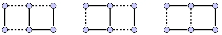
Figure 3.1Three co-path sets (dashed edges), including one of minimum size (rightmost).

k-CO-PATHSET

Input:A graphG= (V,E)and a non-negative integerk. Parameter:k

Problem:Does there existF ⊆E of size exactlyk such thatG[E\F]is a set of disjoint paths?

These problems are naturally motivated by gene mapping, where biologists determine the ordering of genetic markers in DNA using fragment data created by breaking chromosomes with gamma radiation (a technique known asradiation hybrid mapping)[Cox90; RI91; Slo97]. The success of this method depends on being able to construct a linear ordering of the markers based on their co-location on a fragment. Unfortunately, human error in distinguishing markers often means the constraints implied by markers’ co-occurrence on fragments are incompatible with all possible linear orderings, necessitating an algorithm to find the “best” ordering (one which violates the fewest constraints). CO-PATHSETsolves the special case where each DNA fragment contains exactly two genetic markers (corresponding to an edge in the graph); any linear ordering of the markers must correspond to some set of paths, and we minimize the number of unsatisfied constraints (edges in the co-path set).

Recent algorithmic results related to CO-PATHSETinclude two parameterized algorithms decid-ingk-CO-PATHSET[Fen14; Fen15], the faster of which[Fen15]has time complexityO∗(2.17k), and a(10/7)-approximation algorithm[Che11]. However, as written, both parameterized results[Fen14; Fen15]contain a flaw in their analysis which invalidates their probability of a correct solution in the given time1_{. The best known bound prior to}_[_Fen14_]_{is an}_O∗₍_2.45k₎_algorithm_[_Zha14a_]_{. In this} chapter, we prove:

Theorem 1. k-CO-PATHSETis decidable in O∗(1.588k)linear-fpt time with probability at least2/3. We note that standard amplification arguments apply, and Theorem 1 holds for any success probability less than 1. Further, iff is an increasing function with limn→∞f(n) =1, we can solve k-CO-PATHSETwith success probability at leastf(n)inO(1.588knpolylog(n)).

We describe our result in thorough detail in the remainder of this chapter, but will now describe our approach at a high-level to aid with the reader’s intuition. We begin by kernelizing using the

1_{Step 2.11 in both versions of Algorithm R-MCP checks if a candidate co-path set}_F _{has size}

≤k1(as they are sweeping over all possible sizes of candidates and want to restrict the size accordingly). IfF is too large, the algorithm discards it and continues to the next iteration. However, in order for their analysis to hold, the probability that the candidate is contained in a co-path set must be≥(1/2.17)k1_(or(₁/_2.29)k1_in[_Fen14]_{) for}_every_{iteration. Candidates which are too}

(22)

technique from[Fen15], which handles easy cases such as connected components that are cycles and paths, contracts long paths, and applies slightly more technical rules to achieve a kernel. We then make use of a branching technique which yields bounded degree instances. The restrictive structure of path forests enables efficient branching. As part of branching, we delete any instances where more thank edges were removed, and then we pass the remaining instances to our application of the Cut&Count framework. Cut&Count[Cyg11a]is a general framework used for solving decision problems where there is a global constraint. It requires bounded treewidth and uses dynamic programming over a tree decomposition. The key idea is that when building potential solutions in the natural way via dynamic programming, the framework guarantees that non-path forests are seen an even number of times. Then we can count the number of times a potential solution is seen modulto two and obtain a guaranteed “no" if no solution exists and a “yes" with high probability if one does (this is via a one-sided Monte Carlo method). This naturally leads to our result in Theorem 1.

The remainder of this chapter is organized as follows: after essential definitions and notation in Section 3.2, we start in Section 3.3 by giving a newO∗₍₄t w(G)₎_algorithm

tw-copath

_{for solving} CO-PATHSETparameterized by treewidth (tw) using the Cut&Count framework[Cyg11a]. Finally, Section 3.4 describes the linear-fpt algorithm referenced in Theorem 1, which solvesk-CO-PATHSET on general graphs inO∗₍_1.588k₎_{by applying}

tw-copath

_{to a set of “reduced instances” generated} via kernelization and a branching procedure2

deg-branch

_.

3.2

Preliminaries

3.2.1 Treewidth

Our

tw-copath

algorithm in Section 3.3 uses dynamic programming over atree decomposition, and its running time depends on the related measure oftreewidth[Rob86], which we denotetw(G). Treewidth is a measure of how “tree-like" a graph is, with having small treewidth implying being closer to a graph. In order to comprehend the notion of treewidth, an understanding of tree decom-positions is first necessary. Tree decomdecom-positions were originally associated with the graph minor theorem[Rob86].

3.2.2 Tree Decompositions

Atree decomposition[Rob84]of a graphG(V,E)is a pairing of a treeT and a set of bagsX =

{X1, ...,Xn}, where a bag is a subset ofV. The nodes ofT are exactly the bags inX. The following constraints must hold:

1. Everyv∈V must be in at least one bag

2. For everyu v∈E,uandv must be in a common bag

3. For every bagbon a path from bagato bagc inT,a∩c∈b.

(23)

Note that we assume our tree decompositions are rooted, which can be done by arbitrarily selecting a bag to be the root. Thewidthof a tree decomposition is the size of the largest bag (in terms of number of vertices in the bag) minus 1.Treewidthof a graphG is the minimum width of a tree decomposition ofG.

We utilize an enhanced version of tree decompositions,nice tree decompositions[Klo94]. In this paper, anice tree decompositionis a rooted tree decomposition where each node of the tree is one of five specific types:

• Leaf node: Has no children in the tree and contains no vertices.

• Introduce vertex node: Has one child and contains exactly the same vertices as the child plus an additional vertexv. Such a bag introducesv.

• Introduce edge node: Has one child and contains exactly the same vertices as the child. They are labeled with an edgeu v ∈E, whereuandv are contained in the bag. This node is said to introduceu v. We require each edge inE is introduced exactly once.

• Forget vertex node: Has one child and contains exactly the same vertices as the child, with the exception of one single vertexw. Such a bag forgetsw.

• Join node: Contains the exact same vertices as it’s two children,y andz, who contain the exact same vertices as each other.

Note that by the definition oftree decomposition, once a vertex is forgotten, it will not be found further up in the tree. Thus, a vertex is forgotten exactly once. Additionally, we enforce that the root node is of type “forget vertex” (and thus has an empty bag).

Transitioning from a tree decomposition to a nice tree decomposition does not increase treewidth, as we can carry out the transformation by simply adding intermediate nodes between the bags of the original tree decomposition. This transition can be done in polynomial time with respect to the size of the input graph[Cyg11a]. Using nice tree decompositions simplifies finding a dynamic programming algorithm which computes values over the tree decomposition, as there are a finite number of cases to consider.

While explaining our dynamic programming algorithm we also use Iverson’s bracket notation. That is if p is a predicate we let[p]be 1 if p is true and 0 otherwise[Cyg11a]. We view the value of[p] as a multiplicative factor when it precedes an equation or expression. We also use the shorthand

f[x→y]to denote updating a functionf so thatf(x) =y and all other values are unchanged.

3.2.3 Fast Subset Convolution

(24)

rely on uses theZpproduct, which is defined below. We writeZBp for the set of all vectorst of length

|B|assigning a valuet(b)∈Zpto each element ofb∈B.

Definition 2(Zpproduct). Let p≥2be a fixed integer and let B be a finite set. For t1,t2,t ∈ZBp we say that t₁+t₂=t if t₁(b) +t₂(b) =t(b)(inZp) for all b ∈B . For a ring R and functions f,g:ZpB→R , define theZpproduct,∗

p xas

(f ∗pxg)(t) =

P

t1+t2=t

f(t1)g(t2).

Fast subset convolution guarantees that certainZpproducts can be computed quickly.

Lemma 1(Cygan et al.[Cyg11a]). Let R=Zor R=Zqfor some constant q. TheZ4product of functions

f,g :Z4B→R can be computed in4|B||B|O(1)time and4|B||B|O(1)ring operations.

3.3

An

O

∗

(

4

t w(G)

)

Algorithm via Cut&Count

We start by giving an fpt algorithm for CO-PATH SETparameterized by treewidth. Our primary tool is the Cut&Count framework, which enablesct w_nO(1)_{one-sided Monte Carlo algorithms for}

connectivity-type problems with constant probability of a false negative. Cut&Count has previously been used to improve the best-known bounds for several well-studied problems, including CON

-NECTEDVERTEXCOVER, HAMILTONIANCYCLE, and FEEDBACKVERTEXSET[Cyg11a]. Pilipczuk showed that anO∗(ct w)algorithm for some constantc can be designed with the Cut&Count approach for CO-PATHSETbecause the problem can be expressed in the specialized graph logic known as ECML+C[Cyg11b]. However, since our end goal is to improve on existing algorithms fork-CO-PATH SETin general graphs using a bounded treewidth kernel, we need to develop a specialized dynamic programming algorithm with a small value ofc. We show:

Theorem 2. There exists a one-sided fpt Monte Carlo algorithm

tw-copath

deciding k-CO-PATHSET for all k in a graph G in O∗₍₄t w(G)₎_{time with failure probability}_≤₁_/₃_{, when a tree decomposition of} widthtwis given as input.

The Cut&Count technique has two main ingredients: (i) an algebraic approach to counting which uses arithmetic inZ2(enabling faster algorithms) alongside a guarantee that undesirable

objects are seen an even number of times (so a non-zero result implies a desired solution has been seen), and (ii) the idea of defining the problem’s connectivity requirement through consistent cuts. In this context, aconsistent cutis a partitioning(V1,V2)of the vertices of a graph into two sets such

(25)

of subgraphs with consistent cuts which adhere to specific properties pertaining to CO-PATHSET, employs dynamic programming over a nice tree decomposition. We further use weights and the Isolation Lemma to bound the probability of a false negative arising from multiple valid markings of a solution. We use fast subset convolution[Bjö07]to reduce the complexity required for handling join bags in the dynamic programming. In the remainder of this section, we present the specifics for applying these techniques to solve CO-PATHSET.

In order to provide intuition, consider the following example; a graph with two connected components which are bothC4s (cycles on four vertices). For simplicity, we ignore the fact that such

components would be handled by a kernelization step in our approach. Here, ifk=2, it is clear that a solution exists (delete one edge from each cycle), but the answer is no whenk=1. We will point back to this example throughout the following sections.

3.3.1 Cutting

We first provide formal definitions of markers and marked consistent cuts, which we use to ensure that path forests are counted exactly once during our dynamic programming.

Definition 3. A triple(V1,V2,M)is amarked consistent cutof a graph G if (V1,V2)is a consistent cut

and M⊆E(G[V₁]). We refer to the edges in M as themarkers. A marker set isproperif it contains at least one edge in each connected component of G which is not an isolate.

Note that if a marked consistent cut contains a proper marker set, all vertices are on theV1side

of the cut. This is because by the definition of a consistent cut, all isolates are on theV1side, and if

every connected component contains a marker then all connected components must fall entirely on theV1side as well. Therefore for any proper marker set there exists exactly one consistent cut,

while all marker sets which are not proper will be paired with an even number of consistent cuts because unmarked components may lie inV₁orV₂. We use proper marker sets to distinguish desired subgraphs by assigning markers in such a way that when we prune the dynamic programming table for solutions (as described later in the section), the only subgraphs we consider which may have a proper marker set are path forests. We know because the marker set is proper that the subgraph has a unique consistent cut, and thus these path forests will only be counted once in some entry of the dynamic programming table, while all other subgraphs will be counted an even number of times. Note that we are not claiming that all path forests will have proper marker sets. From our earlier example, ifk=2, there will be a setting where we assign one marker to each connected component and there is only consistent cut (both components inV1). Ifk=1, we will only assign a marker to one

component and the second could exist on either side of the cut, and thus there are two consistent cuts in this setting. This is what allows us to do our counting modulo two, as odd total counts imply the existence of a solution.

(26)

four-vertex paths, and is marked when the proper marker set has size two. While cc-solutions can be viewed as solutions due to their complementary nature, being marked is crucial in our counting algorithm and thus subgraphs which are marked-cc-solutions are what correspond to solutions in the dynamic programming table.

We now describe our use of the Isolation Lemma, which guarantees we are able to use parity to distinguish solutions. Letf(X)denoteP

x∈X f(x).

Isolation Lemma 1([Mul87]). LetF ⊆2U _{be a non-empty set family over universe U . A function}

ω:U →Zis said toisolateF if there is a unique S∈ F withω(S) =minF∈Fω(F). Assign weights

ω:U → {1, 2, ...,N}uniformly at random, where the value of N is of the reader’s choice. Then the probability thatωisolatesF is at least1− |U|/N .

Intuitively, ifF is the set of solutions (or complements of solutions) to an instance of CO-PATH SETand|F |is even, then

tw-copath

would return a false negative. This is because while each solution is counted an odd number of times in

tw-copath

, because there are an even number of solutions, the total count of solutions is even, making the combined count of solutions and non-solutions even and the algorithm would incorrectly determine a solution does not exist (a false negative). From our earlier example, there are sixteen valid solutions whenk=2 as we could remove one edge from each cycle, pairwise. Thus, while each solution would be counted once, our total count would still be even. The Isolation Lemma allows us to partitionF based on the weight of each solution (as assigned byω), and guarantees at least one of the partition’s blocks has odd size with constant probability. We letU contain two copies of every edgee ∈E: one representinge as a marker and one as an edge in the cc-solution. Then 2U denotes all pairs of edge subsets (potential marked-cc-solutions), and we setN=3|U|=6E (selected to achieve success probability in Theorem 1). Each copy of an edge is assigned a weight in[1,N]uniformly at random byωand the probability of finding an isolatingωis thus 2/3. We denote the values assigned byωto the set of marker copies byωM, and likewise to the set of edge-in-cc-solution copies byωE.

3.3.2 Counting

A marked-cc-solutionC of a graphG corresponds to a co-path set of sizek when the number of edges and markers inC match specific values which depend onk and|E(G)|. These values are easily deduced because we know the deletion of a co-path set solution of sizek will leave

|E(G)| −k edges in a cc-solution. Furthermore, because a forest hasn−mconnected components, the number of markers inC needs to be at most|V(C)| − |E(G)|+k. All isolates from a forest can be removed and the resulting graph is still a forest, and thus the actual number of markers necessary inC is|V(C)| −nI(C)− |E(G)|+k. From our earlier example, the number of edges whenk =2 is

|E(G)|−k =8−2=6 and the number of markers necessary is|V(C)|−nI(C)−|E(G)|+k=8−0−8+2=2, which we point out is the number of connected components in the aforementioned cc-solution.

(27)

a fixedk). Since no-instances have no appropriately sized marked-cc-solutions, and yes-instances have at least one, odd parity for the number of marked-cc-solutions of size corresponding tok implies a solution to thek-CO-PATHSETinstance must exist.

During the DP algorithm we actually count (for all values(m,e)) the number ofcc-candidates, which are subgraphsG0⊆G with maximum degree 2, exactlye edges, and a marked consistent cut withm markers. The following lemma justifies counting cc-candidates in place of marked-cc-solutions. Note that the weight of a marked-cc-solution or a cc-candidate is equal to the sum of its marker weights and its edge weights.

Lemma 2. The parity of the number of marked-cc-solutions in G with e edges and weight w is the same as the parity of the number of cc-candidates G0⊆G with e edges,|V(G0)| −e−nI(G0)markers, and weight w .

Proof. Consider a subgraphG0⊆G with maximum degree 2 ande edges. LetM0be a marking ofG0 such thatωE(E(G0)) +ωM(M0) =w. Assume first thatG0is a collection of paths. We know thatG0 has|V(G0)| −e−nI(G0)non-isolate connected components. IfM0is a proper marker set ofG0, then

|M0|=|V(G0)|−e−nI(G0)and(G0,M0)has exactly one consistent cut. Therefore(G0,M0)contributes one to both the number of marked-cc-solutions and the number of cc-candidates, respectively.

If otherwiseM0is not a proper marker set, then(G0,M0)contains an unmarked connected component and has an even number of consistent cuts, and therefore contributes an even number to the count of cc-candidates and zero to the number of marked-cc-solutions. Finally, ifG0_contains

at least one cycle thencc(G0)>|V(G0)| −e−nI(G0). Therefore at least one connected component does not contain a marker, and the number of consistent cuts is even, so the contribution to the count of cc-candidates is again even and the contribution to the count of marked-cc-solutions is zero. We conclude that the parity of the number of marked-cc-solutions and the parity of the number of cc-candidates is the same.

Our dynamic programming algorithm is a bottom-up approach over a nice tree decomposition. We build cc-candidates for all values ofmande (encoding the option to add/not add edges and select/not select edges as markers), and keep track of various parameters ensuring that when pruning the DP table we only consider cc-candidates which could be valid solutions to thek-CO -PATHSETinstance. We use the number of edges to ensure our solution is of the correct size, and the number of markers and non-isolate vertices to determine when a subgraph is acyclic. The weight parameter allows us to distinguish between solutions and decreases the likelihood of a false negative occurring via the Isolation Lemma.

Finally, we need a parameter that encodes the degree information required to properly combine cc-candidates as we iterate up the tree. We call this parameter adegree-functionand define it on the verticesV of a bag asf :V →Σ={0, 11, 12, 2}, wheref(v)corresponds tov’s degree in the associated

cc-candidates of the table entry — for vertices of degree 1, their value 1j denotes which side of the partition(V1,V2)they are on. Vertices with degree 0 are on theV1side of the cut by definition and

(28)

Table 3.1Dynamic programming table parameters and upper bounds.

Variable Parameter Maximum value

a # of non-isolated vertices n

e # of edges n2

m # of markers n2

w weight of edges and markers 4n4

cut. In summary, we have table entriesAx(a,e,m,w,s)counting the number of cc-candidates with anon-isolated vertices,e edges,mmarkers, weightw, and degree-functions, where all vertices which have been introduced in the subtree rooted atx are present and only edges which have been introduced in this subtree may be present.

In the following description of the dynamic programming algorithm over a nice tree decomposi-tionT, we letz1,z2denote the children of a join node; otherwise, the unique child is denotedy.

Leaf:

A_x(0, 0, 0, 0,;) =1;A_x(a,e,m,w,s) =0 for all other inputs.

Introduce vertexv:

A_x(a,e,m,w,s[v→0]) =A_y(a,e,m,w,s);A_x(a,e,m,w,s[v→i]) =0, ∀i6=0.

Introduce edgeu v:

Ax(a,e,m,w,s) =Ay(a,e,m,w,s) +

X

αt∈subs(s(t)) t∈{u,v}

¹φ2(αu,αv)ºAy(a

0_,_e₋_1,_m_,_w0_,_s0₎

+X

αt∈subs(s(t)) t∈{u,v}

¹φ1(αu,αv)º

Ay(a0,e−1,m,w0,s0) +Ay(a0,e−1,m−1,w00,s0)

,

whereφj(αu,αv) = (αu =1j ∨s(u) =1j)∧(αv =1j ∨s(v) =1j),a0=a−(|{11, 12} ∩ {s(u),s(v)}|),

w0₌_w₋_ω

E(u v),w00 =w−ωE(u v)−ωM(u v),s0=s[u →αu,v →αv], and thesubsfunction returns all the values the degree-function in child nodey could have assigned to verticesuandv based on current degree-functions (summarized below).

s(v) 0 11 12 2

subs(s(v)) ; 0 0 {11, 12}

(29)

andvhave the appropriatesubsvalues (preventing us from ever having a vertex with degree greater than 2). Note that we use theφjfunction to guarantee that ifslabelsuorvas an isolate, we do not use the introduced edge. We have a summation for both possiblejvalues in order to consideru vfalling on either side of the cut. The formulation ofa0assures that each endpoint of degree 1 is now included in the count of non-isolates (i.e. whenuand/orvhad degree 0 iny). We utilize the marker weight of u v to distinguish when we choose it as a marker (only if onV1side of cut), and incrementm

accord-ingly. In either case, we updatew appropriately (withw0if no marker,w00if marker introduced). Forget vertexh:

Ax(a,e,m,w,s) =

X

α∈{0,11,12,2}

Ay(a,e,m,w,s[h→α]).

As a forgotten vertex can have degree 0, 1 or 2 in a cc-candidate, we must consider all possible values thats assigns tohin child bagy. Note that cc-candidates in whichhis both not an isolate and not a member of a connected component that contains a marker will cancel modulo two, ash can be on either side of the cut and all parameters will be identical.

Join:

We computeA_xfromA_z₁andA_z₂via fast subset convolution[Bjö07]taking care to only combine table entries whose degree-functions arecompatible, ensuring that only joins which preserve the constraints of the degree-functions of the children nodes occur. For example, if a vertexv has been assigned to different sides of the cut inAz1 andAz2, or a total degree greater than two overAz1and Az2, then the degree-functions are incompatible becausevcannot be on both sides of the cut or have total degree greater than two. Similarly, the value it is assigned by the degree-function inAx must accurately correspond to the values inAz1andAz2.

Definition 4. At a join node x with children z1 and z2, the degree-functions s1from Az1,s2from Az2, and s from Ax arecompatibleif one of the following holds for every vertex v in x : (i) si(v) = 0and sl(v) =s(v),i6=l or (ii) s1(v) =s2(v) =1j and s(v) =2for i,j,l∈[1, 2].

In order to apply Lemma 1, we letBbe the bag atx, and transform the values assigned by the degree functions to values inZ4. Letφ:{0, 11, 12, 2} →Z4andρ:{0, 11, 12, 2} →Zbe defined as in

the table below, extending to vectors by component-wise application.

0 11 12 2

φ 0 1 3 2

ρ 0 1 1 2

We use φto apply Lemma 1, while the functionρ (which corresponds to a vertex’s degree) is used in tandem to ensure the compatibility requirements are met: ifφ(s1) +φ(s2) =φ(s), then

necessarilyρ(s1) +ρ(s2)≥ρ(s). From the above table it is easy to verify thatφ(s1) +φ(s2) =φ(s)

andρ(s1) +ρ(s2) =ρ(s)together imply thats1,s2andsare compatible. We sum over both functions

(30)

Assignt1=φ(s1),t2=φ(s2), andt =φ(s)in accordance with Lemma 1. Letρ(s) = P

v∈Bρ(s(v)); that isρ(s)is the sum of the degrees of all the vertices in the join node, as assigned by degree-function s. By defining functions f andgas follows:

f〈d,a,e,m,w〉(φ(s)) =¹ρ(s) =dºAz1(a,e,m,w,s),

g〈d,a,e,m,w〉(φ(s)) =_¹ρ(s) =d_ºAz2(a,e,m,w,s),

and writingr~ifor the vector〈di,ai,ei,mi,wi〉in order to consider all ways to split the parameter values ofx between the two children nodes, we can now compute

Ax(a,e,m,w,s) =

X

~

r1+r~2=〈ρ(s),a0,e,m,w〉 (fr~1_∗4

xg~ r2)(φ(_s))

wherea0=a+|s₁−1{11, 12} ∩s2−1{11, 12}|. We point out that

X

~

r1+r~2=〈ρ(s),a0,e,m,w〉 (fr~1_∗4

xg~

r2)(φ(_s)) =₁

only if bothφ(s1) +φ(s2) =φ(s)andρ(s1) +ρ(s2) =ρ(s); that is, exactly whens1,s2ands are

com-patible.

We conclude this section by describing how we search the DP table for marked-cc-solutions at the root noder. By Lemma 2, the parity of the number of marked-cc-solutions with|E| −k edges and weightw is the same as the parity of the number of cc-candidatesG0_with_|_E_{| −}_k _edges,

|V(G0)| −(|E| −k)−nI(G0)markers and weightw. These candidates are recorded in the table entries Ar(a,|E| −k,a− |E|+k,w,;), whereais the number of non-isolates. Therefore, if there exists some aandw so thatA_r(a,|E| −k,a− |E|+k,w,;) =1, then we have a yes-instance ofk-CO-PATHSET. Note that the degree-function is;in this entry because there are no vertices contained in the root node by definition.

By Lemma 1, the time complexity of

tw-copath

for a join nodeBisO∗₍₄|B|₎_{, which is}_O∗₍₄t w₎_. Note that for the other four types of bags, as we only consider one instance ofsper table entry, the complexity for each isO∗(4t w). We point out that the size of the table is polynomial innbecause there are a linear number of bags and a polynomial number of entries (combinations of parame-ters) for each bag. Since the nice tree decomposition has size linear inn, the bottom-up dynamic programming runs in total timeO∗(4t w). This complexity bound combined with the correctness of

tw-copath

discussed above proves Theorem 2.

3.4

Achieving

O

∗

(

1.588

k

)

in General Graphs

(31)

subgraphs of the input graphG. Specifically, we begin by constructing a kernel of size at most 6k as described in[Fen15]. Our reduced instances are bounded degree subgraphs of the kernel given by a branching technique. We prove that (1) at least one reduced instance is an equivalent instance; (2) we can bound the number of reduced instances; and (3) each reduced instance has bounded treewidth. Finally, we analyze the overall computational complexity of this process.

3.4.1 Kernelization and Branching

We start by describing our branching procedure

deg-branch

(Algorithm 1), which uses a degree-bounding technique similar to that of Zhang et al.[Zha14a]. Our implementation takes an instance (G,k)of CO-PATHSETand two non-negative integers`andD, and returns a set of reduced instances

{(Gi,k−`)}so that (1) eachGiis a subgraph ofG with exactly|E| −`edges and maximum degree at mostD; and (2) at least one(Gi,k−`)is an equivalent instance to(G,k). The size of the output (and hence the running time) of

deg-branch

depends on both input parameters`andD. We will selectD to achieve the desired complexity in

copath

in Section 3.4.3. We also make use of a budget parameterb, which keeps track of how many more edges can be removed per the constraints of` (b is initially set to`).

Our branching procedure leverages the observation that if a co-path setS exists, then every vertex has at most two incident edges not inS. Specifically, for every vertex of degree greater thanD, we branch on pairs of incident edges which could remain after removing a valid co-path set (calling each pair acandidate), creating a search tree of subgraphs.

Algorithm 1:Generating reduced instances

1 Algorithm

deg-branch(G

,k,`,D,b

)

2 Letv be a vertex of maximum degree inG 3 ifd e g(v)≥D+1 andb≥D−1then

4 Arbitrarily select verticesu₁, . . .u_D+₁fromN(v)

5 R=;,E_v={{v,u_i}|i∈[1,D+1]}

6 fore1,e2∈Ev,e16=e2do

7 E_v0=E_v\ {e₁,e₂}

8 R=R∪

deg-branch(G

\E_v0,k,`,D,b−(D−1)

)

9 returnR

10 else ifb=0 andd e g(v)≤D then return{(G,k−`)}

11 else return;

// Discard

G

(32)

Table 3.2Numerically obtained constantscd, 3≤d ≤17, used in Lemma 4; originally given in Table 6.1

of[Gas10].

d 3 4 5 6 7 8 9 10

cd 0.1667 0.3334 0.4334 0.5112 0.5699 0.6163 0.6538 0.6847

d 11 12 13 14 15 16 17

cd 0.7105 0.7325 0.7514 0.7678 0.7822 0.7949 0.8062

size of this set.

Lemma 3. Let T be a search tree formed by

deg-branch

(G,`,D,k,b). The number of leaves of T is at most D₂+1`/(D−1).

Proof of Lemma 3. The number of children of each interior node ofT is D₂+1, resulting in at most D+1

2

d e p t h(T)

leaves. The depth ofT is limited by the second condition of the

if

on line 3 of Algorithm 1. For each recursive call,bis decremented by(D−1), untilb≤D−1. Asbis initially set to`, this impliesd e p t h(T)≤`/(D−1), proving the claim.

Finally, we argue that at least one member of the set of reduced instances returned by

deg-branch

is equivalent to the original. Consider a solutionF tok-CO-PATHSETin the original instance(G,k). Every vertex has at most two incident edges inG[E\F], and since all candidates are considered at every high-degree vertex, at least one branch correctly keeps all of these edges.

3.4.2 Treewidth of Reduced Instances

Our algorithm

deg-branch

produces reduced instances with bounded degree; in order to bound their treewidth, we make use of the following result, which originated from Lemma 1 in[Fom09] and was extended in[Gas10].

Lemma 4. Forε >0, there exists n_ε∈Z+s.t. for every graph G with n>nεvertices,

tw≤ ₁₇

X

i=3

cini

+n_≥18+εn,

where niis the number of vertices of degree i in G for i∈ {3, . . . , 17}, n≥18is the number of vertices of

degree at least 18, and c_iis given in Table 3.2. Moreover, a tree decomposition of the corresponding width can be constructed in polynomial time in n .

(33)

Lemma 5. Let ni be the number of vertices of degree i in a graph G for any i∈Z+, and∆be the

maximum degree of G . If(G,k)is a yes-instance of k-CO-PATHSET, then n3≤2k−( P∆

i=4(i−2)ni). Proof. Since(G,k)is a yes-instance, removing some set of≤k edges results in a graph of maxi-mum degree 2. For a vertex of degreej ≥3, at least j−2 incident edges must be removed. Thus, n3+2n4+3n5+. . .+(∆−2)n∆≤2k(each removed edge counts twice – once for each endpoint).

Lemma 6. Let(G,k)be an instance of k-CO-PATHSETsuch that G has n vertices and max degree at most∆∈ {3, . . . , 17}. If(G,k)is a yes-instance, then the treewidth of G is upper bounded by k/3+εn+c , for anyε >0and constant c =n_εas defined in Lemma 4. A tree decomposition of the corresponding width can be constructed in polynomial time in n .

Proof. Letn_εbe defined as in Lemma 4. LetG0_{be the graph formed by adding}_N ₌_n

εisolates toG. By

Lemma 4, becauseG0has maximum degree at most∆,tw(G0)≤(1/6)n3+(1/3)n4+. . .+c∆n∆+ε(N+n). We can substitute the bound forn₃from Lemma 5, which yields:

tw(G0)≤2k−( P∆

i=4(i−2)ni)

6 +

n4

3 +. . .+c∆n∆+ε(N+n)

≤k

3+ε(n+N).

Note that the inequality holds because we can pair the negative terms of(P∆_i₌₄(i−2)ni)/6 with the corresponding terms ofn4/3+. . .+c∆n∆and the value ofcjnj−(j−2)(nj)/6 is non-positive for all j∈[4, 17]. SinceN =n_εis a constant, we havetw(G0₎_≤_k_/₃₊_ε_n₊_c_{. Since}_G _⊆_G0_{and treewidth is}

monotone under subgraph inclusion, this proves the claim.

We point out that when applying Lemma 6 to reduced instances, computing the desired tree decomposition is polynomial ink (since they are subgraphs of a 6k-kernel).

3.4.3 The Algorithm

copath

This section describes how we combine the above techniques to prove Theorem 1. As shown in Algorithm 2, we start by applying

6k-kernel

[Fen15]to findG0, a kernel of size at most 6k; this process deletesk−k0_{edges. We then guess the number of edges}_k

1 ∈ [0,k0]to remove during

branching, and use

deg-branch

to create a set of reduced instancesQk1, each of which havek

0₋_k

1

edges. Note that

deg-branch

considersallpossible reduced instances, and thus if a (cc-)solution exists, it is contained in at least one reduced instance. To ensure the complexity of finding the reduced instances does not dominate the running time, we set the degree boundDof the reduced instances to be 10 (any choice of 10≤D≤17 is valid). By considering all possible values ofk1, we

(34)

Algorithm 2:Decidingk-CO-PATHSET

1 Algorithm

copath (G

,k

)

2 (G0,k0) =

6k-kernel

(G,k)

3 fork1←0tok0do

4 Q_k

1=

deg-branch

(G

0_,_k0_,_k

1, 10,k1) 5 foreach(Gi,k2)∈Qk1do

6 if

tw-copath

(G_i,k₂)then return

true

7 return

false

Proof of Theorem 1. We now analyze the running time of

copath

, as given in Algorithm 2. By Lemma 3, the size of eachQk1 isO(1.561

k1)_{. For each reduced instance}(_G

i,k2)inQk1, we have

tw(G_i)≤k₂/3+ε(6k) +c by Lemma 6.

Applying Theorem 2,

tw-copath

runs in timeO∗(4k2/3+ε6k)_{for each reduced instance}(_G i,k2)

inQk1 (with success probability at least 2/3). Each iteration of the outer

for

loop can then be completed in time

O∗(1.561k1₄k2/3+ε6k) =_O∗(₄k/3+ε6k) =_O∗(_1.588k)_,

where we use thatk₁+k₂=k0_≤_k_{, and choose}_{ε <}₁₀−5_{. Since this loop runs at most}_k₊_{1 times, this is}

also a bound on the overall computational complexity of

copath

. Additionally

copath

is linear-fpt, as the kernelization of[Fen15]isO(n), and the kernel has sizeO(k), avoiding any additional poly(n) complexity from the

tw-copath

subroutine. Note that by Lemma 4 the tree decomposition can be found in polynomial time in the size of the reduced instance. Since reduced instances are subsets of 6k-kernels, the linearity is unaffected because the graph has size polynomial ink.

3.5

Conclusion

We give anO∗(4t w)fpt algorithm for CO-PATHSET. By coupling this with kernelization and branching, we derive anO∗(1.588k)linear-fpt algorithm for decidingk-CO-PATH, significantly improving the previous best-known result ofO∗₍_2.17k₎_{. We believe that the idea of combining a branching algorithm} which guarantees equivalent instances with bounds on the degree sequence from the problem’s constraints can be applied to other problems in order to obtain a bound on the treewidt