Bayesian Methods for Optimal Treatment Allocation and Causal Inference.

ABSTRACT

GUAN, QIAN. Bayesian Methods for Optimal Treatment Allocation and Causal Inference. (Under the direction of Brian J. Reich and Eric B. Laber).

Bayesian methods are widely used to solve practical problems with advantages of flexibility, easily

quantifying model uncertainty and accommodating unobserved variables. In this dissertation, we combine

Bayesian approaches with other statistical methods to estimate the optimal treatment regime for personalized

medicine and deal with the missing data problem in causal inference.

Personalized medicine attempts to improve healthcare while reducing cost by allocating treatment or

resources to individuals based on personalized characteristics, such as genetics, demographic information,

health status, etc. Personalized medicine, related to the idea of dynamic treatment regime (DTR), can be

for-malized as a sequence of decision rules, one per stage of intervention, for how to make treatment decisions

based on the individual’s up-to-date information. The optimal treatment regime is defined as the regime that

optimizes the population level long-term outcome, sometimes also subject to some cost constraint.

Estimat-ing optimal treatment regime can help policy-makers better allocate resources in terms of improvEstimat-ing efficacy

and controlling cost. In the first two chapters, we propose Bayesian policy search methods to address

cost-constrained treatment allocation problems with applications to periodontal recall interval recommendation

and resource allocation for malaria control.

In Chapter 1, we combine non-parametric Bayesian dynamic modeling with policy search algorithm

to estimate the optimal recall interval recommendation regime within a class of interpretable regimes for

patients with periodontal disease. Tooth loss from periodontal disease is a major public health burden in

the United States. Standard clinical practice is to recommend a dental visit every six months; however, this

practice is not evidence-based, and poor dental outcomes and increasing dental insurance premiums indicate

room for improvement. We consider a tailored approach that recommends recall time based on patient

char-acteristics and medical history to minimize disease progression without increasing resource expenditures.

The dynamics of periodontal health, visit frequency, and patient compliance are complex, yet the estimated

restrict our policy search space to a class of interpretable regimes. Both simulation experiments and

appli-cation to a rich database of electronic dental records from the HealthPartners HMO shows that our proposed

method leads to better dental health without increasing the average recommended recall time relative to

competing methods.

In Chapter 2, we develop a framework to help policy-makers decide how to allocate their limited

re-sources in realtime for malaria control. We construct an interpretable class of resource allocation policies

that can accommodate a continuous action space, and combine a hierarchical Bayesian spatiotemporal model

for the disease transmission with the policy search algorithm to estimate the optimal resource allocation

pol-icy within the pre-specified class of policies. The optimal polpol-icy estimated using the proposed framework

improves the cumulative long-term outcome compared with naive policies in both simulation experiments

and application to malaria interventions in the Democratic Republic of the Congo.

After estimating optimal treatment regimes, it is also important to develop a valid inference method to

evaluate average treatment effect. Missing data problem is very common in observational studies, which

brings difficulties in average causal effect estimation. Multiple imputation (MI) that uses a Bayesian

ap-proach to generate imputed values is widely used to handle missing data. The multiple imputation variance

estimator proposed by Rubin is easily applicable, bot not necessarily consistent. In Chapter 3, we establish a

novel martingale representation for MI estimators of the average causal effect, and propose a weighted

boot-strap procedure that can provide asymptotically valid inference regardless of which full sample estimator

is adopted in MI. A comprehensive simulation study shows that the proposed method works well in finite

© Copyright 2019 by Qian Guan

Bayesian Methods for Optimal Treatment Allocation and Causal Inference

by Qian Guan

A dissertation submitted to the Graduate Faculty of North Carolina State University

in partial fulfillment of the requirements for the Degree of

Doctor of Philosophy

Statistics

Raleigh, North Carolina

2019

APPROVED BY:

Brian J. Reich

Co-chair of Advisory Committee

Eric B. Laber

Co-chair of Advisory Committee

Shu Yang Rui Song

DEDICATION

BIOGRAPHY

The author was born in Tongling, Anhui Province, China in 1991. She obtained her bachelor’s degree in

Computational Mathematics in 2013 and another bachelor’s degree in Accounting in 2014 from Sun

Yat-sen University. After that, she continued her study at the Department of Statistics at North Carolina State

University. Under the direction of Dr. Brian Reich, Dr. Eric Laber and Dr. Shu Yang, she will earn her Ph.D.

ACKNOWLEDGEMENTS

First of all, I would like to express my sincerest gratitude to my advisors, Dr. Brian Reich, Dr. Eric Laber and

Dr. Shu Yang for their great mentoring, inspirational ideas and continued support during my Ph.D. study.

They are very smart, knowledgeable and enthusiastic. Whenever I encounter difficulties in the research,

they always patiently give me encouragement and insightful guidance to help me move forward. They do

not only provide valuable research ideas, but also instruct me how to conduct research and improve writing

and presentation skills. I am so lucky to have them as my advisors, without whom I would not come so far.

I would like to thank Dr. Rui Song and Dr. Krishna Pacifici for severing on my committee and providing

insightful comments. I also thank Dr. Wenbin Lu, who serves as current DGP of our department and my

academic advisor during my first year of study, for the valuable guidance and tremendous help he provided.

I would also like to extend my appreciation to all faculty members and staff at the Department of Statistics

for offering so many amazing courses and great services.

I am also grateful to the wonderful internship experiences I have during my Ph.D. study. At Merck,

Dr. Devan Mehrotra and Dr. Zifang Guo not only mentored me on impactful statistical research, but also

provided me with valuable suggestions on career development. At Maxpoint, Yi Chao and Saravana

Srini-vasan shared with me many practical knowledge and skills. At Eli Lilly and Company, Dr. Ran Duan and

Dr. Yongming Qu taught me interesting research ideas and helped me learn better about pharmaceutical

companies.

Last but not least, I want to express my deepest love and gratitude to my family. My parents always

stand by me for the ups and downs in my life and give me unconditional support and love. My husband,

Wenhao Hu, always gives me encouragement and helps me become a better person. We have been through

many good and bad times, and he is always there to be my strength. My lovely daughter, Mia, has brought

TABLE OF CONTENTS

LIST OF TABLES . . . vii

LIST OF FIGURES . . . viii

Chapter 1 Bayesian Nonparametric Policy Search with Application to Periodontal Recall In-tervals . . . 1

1.1 Introduction . . . 1

1.2 HealthPartners Data . . . 4

1.3 Problem Statement . . . 6

1.4 Bayesian Model for Disease Progression . . . 8

1.5 Policy Search . . . 10

1.6 Simulation Studies . . . 13

1.7 Application: HealthPartners Data . . . 19

1.7.1 Tailoring the BNP Model . . . 19

1.7.2 Summarizing the Fitted Model . . . 20

1.7.3 Summarizing the Fitted Policy . . . 20

1.8 Conclusions . . . 24

Chapter 2 A Spatiotemporal Recommendation Engine for Malaria Control. . . 26

2.1 Introduction . . . 26

2.2 Problem Statement . . . 29

2.3 Bayesian Spatiotemporal Model . . . 31

2.4 Recommendation Engine . . . 32

2.4.1 Priority Score . . . 33

2.4.2 Local Utility Function . . . 34

2.4.3 Global Utility Function . . . 35

2.5 Policy Search . . . 36

2.6 Simulation Studies . . . 37

2.6.1 Generative Model . . . 37

2.6.2 Policy Estimation . . . 38

2.7 Application to the DRC Data . . . 41

2.8 Discussion . . . 44

Chapter 3 Novel Bootstrap Inference for Causal Inference with Multiple Imputation . . . 47

3.1 Introduction . . . 47

3.2 Background and Setup . . . 50

3.2.1 Potential Outcomes Framework. . . 50

3.2.2 Common Estimators for the ACE. . . 51

3.2.3 Asymptotically Linear Estimators . . . 53

3.2.4 MI in the Presence of Missing Confounders. . . 54

3.3 Bootstrap Inference for the MI Estimators of Causal Effects . . . 56

3.3.2 Wild Bootstrap for the MI Estimators of the ACE . . . 58

3.4 Missingness not at Random . . . 59

3.5 Simulation . . . 60

3.6 Applications . . . 63

3.7 Conclusion . . . 64

3.8 Proof and Technical Details . . . 64

3.8.1 Assumptions . . . 64

3.8.2 Proof of Theorem 1 . . . 65

References . . . 69

Appendix . . . 85

Appendix A Supplementary Materials for Chapter 1 . . . 86

A.1 Priors and MCMC Details . . . 86

A.1.1 Simulation Studies . . . 86

A.1.2 HP Data Analysis . . . 88

A.2 Additional Simulations . . . 93

A.2.1 Considering Binary Covariates, Quadratic Effects, and Non-constant Variances 93 A.2.2 Comparison with the Overall Oracle Policy in a Simple Setting . . . 94

LIST OF TABLES

Table 1.1 Simulation study results comparing the baseline model with 6-month recommendation for all subjects, policy search methods based on Gaussian and Dirichlet process mixture (DPM) fits, and the oracle model which uses the true data-generating model to estimate the policy. The standard errors of the sample means are all less than 0.01. . . 16 Table 1.2 The posterior mean×100and standard deviation×100for weighted average of random effects

withlog(δit),Y_it?andΦ−1(pit)as responses, respectively. The posterior mean with “?” represents the corresponding95%credible intervals that excludes zero. . . 21 Table 2.1 The posterior mean and 95% credible interval for parameters. The posterior mean with “?”

rep-resents the corresponding95%credible intervals that excludes zero. . . 42 Table 3.1 Point estimates, true variance, relative bias of the variance estimators together with

cov-erages and mean width of interval estimates using Rubin’s method and proposed wild bootstrap method under the scenario where missing at random is assumed. . . 61 Table 3.2 Point estimates, true variance, relative bias of the variance estimators together with

cov-erages and mean width of interval estimates using Rubin’s method and proposed wild bootstrap method under the scenario where missing not at random is assumed. . . 62 Table 3.3 Point estimates, true variance, relative bias of the variance estimators together with

cov-erages and mean width of interval estimates using Rubin’s method and proposed wild bootstrap method under the scenario where the true missing mechanism is missing not at random but missing at random is assumed . . . 63 Table 3.4 Point estimates, the variance of point estimators, and 95% confidence interval estimated

using Rubin’s method and proposed wild bootstrap method. . . 64

Table A.1 Simulation study results comparing the baseline model with 6-month recommendation for all subjects, policy search methods based on Dirichlet process mixture (DPM) fits, and the oracle model which uses the true data-generating model to estimate the policy. . . 96 Table A.2 Validation results comparing six models in terms of mean square error (MSE), mean absolute

LIST OF FIGURES

Figure 1.1 The proportion of sites with unhealthy PPD (pocket depth exceeding 3mm) or missing tooth, denoted by PMU, over time, for 10 randomly chosen subjects. . . 5 Figure 1.2 Density plots of actual time between visits (δmonths) for each level of recommended recall

interval (Amonths). . . 6 Figure 1.3 Illustration of how to optimize a sequence of recall intervals under a given policy using the

proposed method. In this hypothetical example, the risk scoreRtis a linear combination of the

current disease statue (Yt) and a single covariate (X), and the two actions are to return in 3 or 9

months. . . 11 Figure 1.4 Estimated optimal feature weightsαoptfor the simulation study. The boxplots for the Gaussian

and DPM methods show the estimatedαoptover the 100 simulated datasets; the solid points

representαopt for the Oracle policy. The risk score is a linear combination the two baseline

covariates (X1andX2), non-compliance (“Non-comp”;log(|δt−1−At−1|+ 1)), and disease status (“Cur Y”;Yt−1): . . . 17

Figure 1.5 Value and average recommended recall time for the 100 datasets for the policy (viaαopt)

es-timated using the Gaussian model or DPM model for data generated from a two-component mixture model withn= 1,000subjects using reduction utility function. The value and average recommended recall time of the policy are evaluated using Monte Carlo samples under the true model used to generate the data and the estimated Gaussian model or DPM model. . . 18 Figure 1.6 Posterior distribution (5th, 25th, 50th, 75th, 95th percentiles) of optimal feature weightsαoptfor

the HP data analysis. The features are age (standardized), diabetes (with diabetes=1 and without diabetes=0) non-compliance (log(|δt−1−At−1|+ 1)), and current response (Yt−1). . . 23

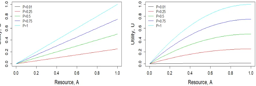
Figure 2.1 Linear (left) and quadratic (right) utility functionU(a, p)as a function of resource al-location a for different values of the priority scores,p. The linear utility function is

U(a, p) = ap and the quadratic utility function is U(a, p) = −p(a−1)2 + p for 0≤a≤1. . . 35 Figure 2.2 The improvement of the proposed policies with linear utility function or quadratic utility

func-tion compared with “Highest rate” policy (left) and “Even” policy (right) with different resource constraintsC= 0.2,0.5and0.8when the model is correctly specified. . . 39 Figure 2.3 The improvement of the proposed policies with linear utility function or quadratic utility

func-tion compared with “Highest rate” policy (left) and “Even” policy (right) with different resource constraintsC= 0.2,0.5and0.8the the model is misspecified. . . 40 Figure 2.4 Posterior distribution (5th, 25th, 50th, 75th, 90th percentiles) of the weightsαoptfor risk

factors and the spatial penalty term when using linear utility function (left) or quadratic utility function (right). The risk factors include temperature (standardized), precipitation (standardized), current disease rate (logit), current neighborhood disease rate (logit). . . 43 Figure 2.5 The resource allocation next year using the estimated optimal policies with either the linear

Figure A.1 Estimated optimal feature weightsαoptfor the simulation study with different sample sizes. The

boxplots show the estimatedαoptover the 100 simulated datasets for sample sizen= 500and

sample sizen= 1000; the solid points representαoptfor the Oracle policy. The risk score is

a linear combination the two baseline covariates (X1andX2), non-compliance (“Non-comp”;

log(|δt−1−At−1|+ 1)), and disease status (“Cur Y”;Yt−1): . . . 93

Figure A.2 Estimated optimal feature weightsαoptfor the simulation study scenario 1, 2 and 3. The

box-plots show the estimatedαoptover the 100 simulated datasets; the solid points representαopt

for the Oracle policy. The risk score is a linear combination the two baseline covariates (X1and X2), non-compliance (“Non-comp”;log(|δt−1−At−1|+ 1)), and disease status (“Cur Y”;Yt−1): 95

Chapter 1

Bayesian Nonparametric Policy Search with

Application to Periodontal Recall Intervals

1.1

Introduction

Periodontal disease (PD) contributes to eventual tooth loss and remains a major health burden. The ultimate

goal of professional periodontal maintenance plans (AAP, 2001) and personal oral care is PD prevention

and maintaining teeth in a state of comfort and function. The total dental healthcare spending in the United

States in 2013 was a staggering US$ 91.8 billion (Wall, Thomas and Guay, Albert, 2016), and is continually

increasing (CDC, 2010). Hence, there is an urgent need to reduce cost without diminishing the quality of

care. In the context of dental care, updating periodontal recall recommendations to reflect the individual

needs of each patient holds the potential to both improve oral health and reduce cost. The length of

peri-odontal recall intervals has been a topic of research and debate for decades (L¨ovdal et al., 1961; Axelsson

et al., 1991; Fardal et al., 2004; Mettes, 2005; Riley et al., 2013) with recommendations for recall intervals

ranging from two weeks (Nyman et al., 1975) to eighteen months (Ros´en et al., 1999). The current standard

of care, which was advocated as early as 1879 by the American Academy of Dental Science (Teich, 2013),

is a recall interval of six months for all patients regardless of individual demographics, oral health, family

on individual patient characteristics (NCCAC, 2004; Patel et al., 2010; see also Giannobile et al., 2013) but

offer little concrete guidance on how to map individual patient characteristics to a recall interval.

The potential effect of altering such intervals on oral health had remained the subject of international

debate for almost three decades (Mettes, 2005; Riley et al., 2013). Infrequent dental visits might impair

the ability to diagnose PD at an early stage, present fewer opportunities for providing oral-care education,

and block opportunities for effective treatments (Davenport et al., 2003). However, unnecessary visits and

treatments waste resources and increase cost. Therefore, the recall interval should be tailored to

individ-ual needs. Patients at high risk may benefit from more frequent visits while less frequent visits might be

adequate for subjects without certain risk factors of PD (Giannobile et al., 2013). This provides evidence

that a personalized (or precision) medicine approach (Kornman and Duff, 2012; Zanardi et al., 2012) might

improve resource allocation for preventive dentistry.

In this chapter, we consider adaptive recall intervals that recommend a recall time for each patient at

each visit depending on their personal characteristics, including disease history. We formalize a personalized

recall interval policy as a function that maps current patient information to a recommended recall interval,

which is an example of a dynamic treatment regime, or DTR (Murphy, 2003a; Robins, 2004; Chakraborty

and Moodie, 2013; Schulte et al., 2014; Laber et al., 2014b; Kosorok and Moodie, 2015). An optimal DTR

is a sequence of decision rules that maps an individual’s current information to a recommended treatment to

maximize long-term population-level benefit. The problem we are addressing is to establish a rule for giving

recall recommendations based on a patients’ demographic information and periodontal treatment history to

maximize the population five-year average reduction in periodontal disease, and is thus a DTR problem.

DTRs have been applied across a wide range of application domains to estimate data-driven intervention

policies (van der Laan and Petersen, 2007; Robins et al., 2008; Shortreed and Moodie, 2012; Laber et al.,

2014b; Almirall et al., 2014; Wu et al., 2015); however, estimation of an optimal recall intervention policy

presents several challenges that make existing estimation methods unsuitable without modification. These

challenges include: (i) cost constraints on recall frequency across the entire population; (ii) non-compliance

and sparse irregularly spaced clinic visits; (iii) a bounded response with a large point mass on the response

them; and (iv) the requirement that the estimated policy be clinically interpretable, despite complex disease

dynamics. Existing methods for cost-constrained DTRs include cost-constrained IQ-learning (Linn et al.,

2016) which only applies for two decision points; cost-sensitive DTRs (Luedtke and van der Laan, 2016)

which constrain the proportion of individuals who can receive treatment; set-valued DTRs (Laber et al.,

2014a; Lizotte and Laber, 2016) which allow for multivariate outcomes, e.g., cost and efficacy, but do not

permit constrained estimation. Functional and longitudinal methods for DTRs can accommodate sparse

and irregularly-spaced observation times (Ciarleglio et al., 2015; Lu et al., 2016; Laber and Staicu, 2016),

however, these methods are not designed for application with many, possibly outcome-driven, follow-up

times, nor can they deal with non-compliance.

Policy-search is a common method for estimation of a DTR, and is particularly well-suited to

con-strained problems (Chakraborty and Moodie, 2013; Wang et al., 2018; Laber et al., 2018b). Policy-search

methods postulate a model for the marginal mean outcome under each policy within a pre-specified class

of policies and choose the maximizer as the estimated optimal policy (Robins et al., 2008; Orellana et al.,

2010; Zhang et al., 012a,b; Zhao et al., 2012; Zhang et al., 2013; Zhao et al., 2015; Kosorok and Moodie,

2015; Guan et al., 2016; Zhou and Kosorok, 2017). An advantage of policy-search methods is that models

for the underlying disease progression can be decoupled from the class of policies, thereby allowing for

complex disease models with parsimonious, interpretable, or cost-constrained estimated optimal policies

(Zhang et al., 2015; Laber and Zhao, 2015; Lakkaraju and Rudin, 2016). However, existing methods for

policy-search are difficult to implement for complex data structures, like the one we consider here.

We use a Bayesian nonparametric (BNP) disease dynamics model and g-computation (Robins, 1986)

to construct an estimator of the marginal mean outcome and cost under any policy within a pre-specified

class, and then use stochastic optimization to approximate the maximizer of the mean outcome under a

constraint on cost. The marginal mean outcome is cumulative, and accounts for disease progression and

delayed effects of treatment. We estimate this marginal mean outcome using g-computation, which accounts

for these effects and other time-varying causal confounding. The proposed dynamics model is sufficiently

flexible to accommodate non-compliance, sparse and irregularly-spaced visits; however, our class of policies

estimating optimal treatment regimes (Arjas and Saarela, 2010; Xu et al., 2016; Murray et al., 2017), but

they did not consider regimes that adapt to the evolving health status of each individual patient, or cost

constraints.

The motivation for establishing this (recall) recommendation engine comes from analyzing an

obser-vational database in a dental practice-based setting, collected by the HealthPartners®(HP) Institute at

Min-neapolis, Minnesota. In Section 1.2, we review the HP data. In Section 2.3, we formalize the recall estimation

problem using a decision theoretic framework. In Section 1.4, we present a BNP formulation of the disease

dynamics and in Section 2.4, we combine this model with a stochastic optimization algorithm to construct

an estimator of the optimal intervention policy subject to constraints on cost. In Section 2.6, we evaluate

the finite sample performance of the proposed methods using a suite of simulation experiments. We analyze

the motivating HP dataset and summarize the fitted policy in Section 1.7. We conclude with a discussion in

Section 1.8.

1.2

HealthPartners Data

The motivating longitudinal HP dataset were collected from routine dental practice in the Minneapolis area.

We include only adult subjects with at least two visits, giving 24,731 subjects with as many as 8 years

of irregular longitudinal follow-up, with an average of 8.6 visits. For each subject, we use the data from

the first visit until the last visit to fit the model proposed in Section 2.3, and so the follow-up window

varies by subject. During each visit, periodontal pocket depth (PPD) is recorded at six pre-specified sites

per tooth (excluding the third molars) giving 168 measurements for a full mouth without any missing tooth.

In concordance with the proposed standards from the joint EU/USA Periodontal Working Group (Holtfreter

et al., 2015), we use the proportion of diseased/affected tooth sites (with PPD >3mm, or missing tooth)

per mouth, henceforth PMU, as our response to measure the extent (severity) of PD. Note, when the tooth

is missing, we assume the missingness is due to PD and we classify all sites associated with the missing

tooth are diseased tooth sites so each missing tooth contributes to 6 diseased tooth sites in the calculation.

Demographic information and medical history are also collected, including age (ranging from 19 to 97 years,

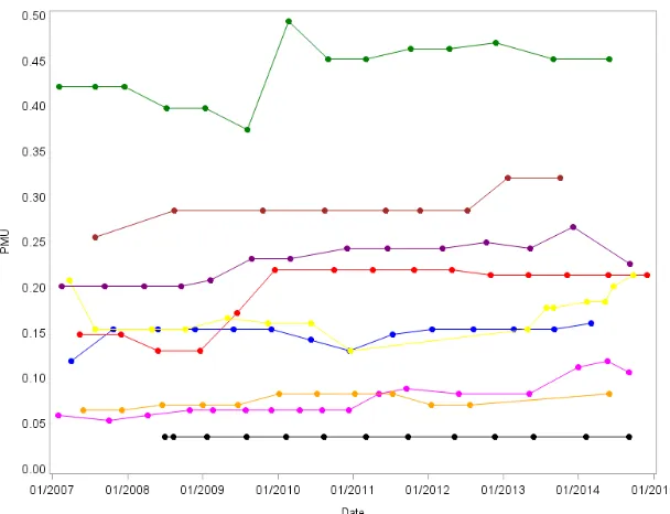
Figure 1.1: The proportion of sites with unhealthy PPD (pocket depth exceeding 3mm) or missing tooth, denoted by PMU, over time, for 10 randomly chosen subjects.

(8% with diabetes, 92% without diabetes), smoking status (9% current tobacco user, 91% not current user),

and insurance information (80% with commercial insurance, 20% without commercial insurance).

Figure 1.1 plots the longitudinal profiles for 10 subjects. Although there are some short-term decreases,

there is a clear population-level increasing trend. A high proportion of the responses are identical to the

pre-vious response, reflecting the common practice of carrying the prepre-vious values forward in the dental record

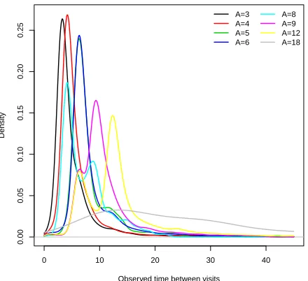
if there is no apparent change in disease status. During each visit, the recommended time until the next visit

(A) is also recorded, and the actual time between two visits (δ) is computed. HP uses an algorithm to classify

subjects as low, medium or high risk of PD and caries, and this risk score is taken into consideration when

recommending the next visit time. However, this risk score is not optimized for recall recommendations,

and dentists are not obliged to use it. The range ofA, as indicated in Figure 1.2, varies significantly from

3 months to 18 months. The figure also illustrates the partial controllability, with a strong but imperfect

0 10 20 30 40

0.00

0.05

0.10

0.15

0.20

0.25

Observed time between visits

Density

A=3 A=4 A=5 A=6

A=8 A=9 A=12 A=18

Figure 1.2: Density plots of actual time between visits (δmonths) for each level of recommended recall interval (A months).

1.3

Problem Statement

The data at baseline for subjecti= 1, . . . , ninclude thep-vector of covariates,Xiand the scalar baseline response,Yi0. At the baseline visit, a recommended number of months until the first follow-up visitAi1 >

0 is given. The subject returns for the first following visit δi1 > 0 months after the baseline visit, and

the subject’s response, Yi1, is recorded. This process is repeated forNi follow-up visits for the subjecti.

The data available after visittfor subjectiareHit = {Xi, Yi0, Ai1, δi1, Yi1, . . . , Aiti, δit, Yit}, andHi ≡

HiNi is the entire history for subjecti. The subscriptiis suppressed to denote a generic trajectoryHt =

{X, Y0, A1, δ1, Y1, . . . , At, δt, Yt}.

Our objective is to use these data to determine a policy for recommending the time between visits. A

policyπis a deterministic function that maps the available data to a recommendation, i.e., underπ,

The policy is parameterized in terms of the unknown vectorα = (α1, . . . , αq)T. For interpretability, we

assume that the policy is a function of a risk score that is a linear combination of features constructed from

Ht,f(Ht) = [f1(Ht), . . . , fq(Ht)]T. There is great flexibility in constructing the features; they can include the covariates themselves,fk(Ht) =Xj, or composites such as change from baselinefk(Ht) =Yt−Y0, or

even summaries of the posterior predictive distribution. The risk score is thenRt=f(Ht)Tα, and subjects with high risk scores are recommended to have smallAt, whereas subjects with low risk are recommended

to a largerAt. While including many features can give a rich class of policies, we consider a small value ofq

so that the subclass of policies is interpretable, and the optimization problem reduces to estimating the

low-dimensional vectorα. We useΠto denote the above pre-specified class of policies that are parameterized

byα.

We formalize the optimal recall interval recommendation policy within the classΠusing potential

out-comes. DefineY_t?(at)andδ?t(at)to be the potential PMU outcome at visittand potential time between visit

tand visitt−1, respectively, if the sequence of recall recommendationsatwould be given to a subject since

baseline visit, whereat = {a1, . . . , at}denotes the history of recall interval recommendations up to visit

t. DefineY?

t(π),δ?t(π)to be the potential outcomes at visittunder recall interval recommendation policy

π. The value associated with a policy can be defined as the expectation of a function of potential outcomes

under the policy, e.g.,V(π) = E{[1/J?(π)]PJ

?_(π)

t=1 Yt?(π)}, where J?(π)is the number of visits within a pre-specified time period under policyπ. The optimal policy within the pre-specified class of policies is

πopt = arg max π∈Π

V(π). In order to estimate the optimal recall interval recommendation policy within the

pre-specified class using the observed data, we make the following assumptions: (1) no unmeasured

con-founders (or sequential ignorability) (Robins, 2004),{(Y_k?(ak), δ_k?(ak)) : for allak ∈ Ak}k≥1 ⊥⊥ At|Ht fort= 1, . . . , N, whereAk =A1× · · · ×Akis the set of all possible recall interval recommendations up to

visitk; (2) consistency,Yt=Y?(At)andδt=δ?(At), whereAtis the sequence of observed recommended

recall intervals up to visitt, i.e., the observed outcomes are the potential outcomes under the actual given

recall interval recommendation; (3) positivity, there exists > 0so thatP(At = at|Ht = ht) ≥ for all

at∈Ψt(ht)and for allht, whereΨt(ht)is the set of possible recall interval recommendations for a subject

optimal policy is causally interpretable (Robins, 2004; Schulte et al., 2014), and we use the notation of the

generic trajectory instead of potential outcomes hereafter.

To compare policies, we use a utility functionU(H), which is considered the primary outcome to be op-timized. Based on the underlying clinical science and logistical constraints, we chose 5-year mean reduction

in the proportion of unhealthy sites as one of our primary outcomes; however, the proposed methodology

can be extended to other time horizons, or other summaries of a patient’s health trajectory. We desire a

policy that applies to all subjects, and we therefore compare the population mean utility, called the value,

V(α) =Eα[U(H)]. The expectation averages over the entire distribution ofH, including the baseline co-variates, the visit times as determined byδt, and the PMU trajectoryY0, . . . , YN. The policy vectorαalters

the value indirectly via the recommendation timesAtwhich subsequently affect the time courses ofδtand

dental health stateYt. Therefore, estimating the value of the policy requires determining compliance

rela-tionship (the distribution ofδtgivenAt), and the effect of recall on PD (the distribution ofYtgivenδt). In

addition to value, policies must be compared in terms of their cost because it is not feasible to recommend a

short time between visits for all subjects. We control cost by constraining the average recommended recall

time to beT,C(α) =Eα(At) =T.

The objective is to identify an α which maximizes the valueV(α) while maintaining cost constraint

C(α) =T. Rather than attempting to estimateαdirectly from the data, our approach is to first estimate the

distribution ofHas a function ofαusing a BNP model (Section 1.4). Given this model, we can then simulate from the process to obtain Monte Carlo estimates ofV(α)andC(α)for anyα, and use this simulation as

a basis for determining the optimalα(Section 2.4).

1.4

Bayesian Model for Disease Progression

For our application, we build a Dirichlet Process Mixture (DPM) model that is parsimonious enough to

fit large data sets and facilitate the extensive simulation required for policy evaluation, yet flexible enough

to capture the complex dynamics of the HP data. Heterogeneity across subjects is captured with subject

random effectsΘi ={θi0,θi1,θi2}that includes random effects for baseline status (θi0), compliance (θi1),

random effects, we propose a Markov outcome-dependent follow-up model (Ryu et al., 2007) forHi,

(XT_i , Yi0)T|Θi ∼ Normal(θi0,Σ0) (1.2) log(δit)|Θi,Xi, Yit−1, Ait ∼ Normal(XitTθi1, σ21)

Yit|Θi,Xi, Yit−1, δit ∼ Normal(ZitTθi2, σ22)

whereXit= [XTi , Yit−1,log(Ait),XTi log(Ait), Yit−1log(Ait)]T andZit= (XTi , Yit−1, δit,XTi δit, Yit−1δit)T. Although this first-stage model is relatively simple, the overall model is flexible when integrated over

the random effects Θi. For example, compliance δit/Ait depends on both covariates and current disease

status, and these relationships are individualized throughθi1. Similarly, the individualized treatment effect

is controlled byθi2and the induced relationship betweenδit,Yit−1, andYit. Also, prior correlation between

θi0 andθi2 can accommodate effect modification between the baseline covariates and time between visits

in the PMU model. Of course, even more flexible models can be constructed using non-linear terms inXit

andZitand higher-order lags in the Markov model.

Let gbe the random effects density, such thatΘi iid∼ g(Θ). Rather than selecting a parametric model

for g, we treat the density as an unknown quantity to be estimated from the data. The prior for g is

modeled using the Dirichlet process prior (Ferguson, 1973; Sethuraman, 1994), which can be written as

g(Θ) = PL

l=1ωl1∆l(Θ), whereL = ∞, the mixture probabilities ωl > 0 satisfy

P∞

l=1ωl = 1, ∆l =

(θ?T_0l ,θ₁?T_l ,θ?T_2l )T ∼Normal(mb,Σb), and1∆l(·)is the indicator function with a point mass at∆l. The

mix-ture probabilities can be generated from the stick-breaking process:ωl=VlQh<l(1−Vh),Vl∼Beta(1, α0).

The covariance matrixΣb is taken to be block diagonal with Cov(θ?jl) = Σbj and Cov(θ?jl,θ?kl) = 0. For

priors, we selectmb∼Normal(0, I)andΣbj ∼InvWishart(pj+ 1,(pj+ 1)Ipj), wherepjis the dimension

ofθ?_jl. With these priors and truncation at a finiteL, all full conditional distributions are conjugate and so

1.5

Policy Search

Although other classes of policies are possible, such as trees (Laber and Zhao, 2015) and lists (Zhang

et al., 2015), we consider policies defined by a linear risk score. Let the risk score be Rt = f(Ht)Tα, wheref(Ht)is aq-vector of features andα = (α1, . . . , αq)T are their weights. Our general framework can easily accommodate non-linear relationships between patient characteristics and the risk score by including

non-linear summaries of the characteristics as features. As an extreme example, we could include B-spline

basis or tree expansion of a variable as features to give an arbitrarily flexible risk score. We could also

include an interaction between a characteristic and disease status to account for different importance of the

characteristic as the disease progresses. However, our goal is to develop a policy that is interpretable to

domain experts so that it can be integrated to the clinical practice. Hence, we decided to keep the risk score

simple. We describe the method assuming two possible recommendations,a1 anda2. The policy takes the

form

At=π(Ht;α) =



  

  

a1 Rt> κ(α)

a2 Rt≤κ(α)

(1.3)

where κ(α) is the risk threshold that depends on α; more than two treatments could be accommodated

using multiple thresholds. With only a single threshold, the scale ofαis irrelevant, and so we impose the

restriction ||α|| = (Pq

j=1α2j)1/2 = 1. Figure 1.3 illustrates how the proposed method is used when a sequence of recall intervals needs to be optimized under a given policy in terms ofα.

We select the policy parametersαso that when the population of patients follows this rule over time, the

long-term average reward is high. Given the posterior of the random effects distribution gand covariance

parametersS ={Σ, σ1, σ2}, the optimal feature weightαis given by

αopt= arg max

α V(α) such that C(α) =T. (1.4)

However, this is a challenging optimization problem, because bothV(α)andC(α) are expectations with

𝑅𝑡 = 𝛼1𝑌𝑡+ 𝛼2𝑋

𝐴𝑡=

3 𝑅𝑡> 0

9 𝑅𝑡< 0 𝑅1>0

Baseline

Recommendation Policy

𝐴1= 3

𝑅1<0

𝐴1= 9

𝑅3>0 𝐴3= 3

𝑅3<0 𝐴3= 9

𝑅3>0 𝐴3= 3

𝑅3<0 𝐴3= 9

𝑅3>0 𝐴3= 3

𝑅3<0 𝐴3= 9

𝑅3>0 𝐴3= 3

𝑅3<0 𝐴3= 9 𝑅2>0

𝐴2= 3

𝑅2<0 _{𝐴2= 9}

𝑅2>0

𝐴2= 3

𝑅2<0 _𝐴 2= 9

Figure 1.3: Illustration of how to optimize a sequence of recall intervals under a given policy using the proposed method. In this hypothetical example, the risk scoreRtis a linear combination of the current disease statue (Yt) and a

single covariate (X), and the two actions are to return in 3 or 9 months.

{g(j),S(j)_{;j = 1, . . . , J}. For each candidateα and κ(α), we simulate subject i = 1, . . . , n}

0 by first

samplingj randomly from{1, . . . , J}, thenΘi ∼ g(j), and finallyHi from (1.2) givenΘi andS(j), with recommendations given by π(Hit;α). Note that in these simulations, the actions taken affect the future outcomes and thus future recommendations, and in this way the method can allow for delayed effects.

For each candidate α, we first identify the thresholdκ(α) that satisfies the cost constraintC(α) ≈

T, and then estimate the valueV(α) given this threshold. We estimate C(α)separately for a grid of 10

thresholds spanning the range ofRtin the training data, smooth the estimates using LOESS (Cleveland and

Devlin, 1988), and then compute theκ that givesC(α) ≈T. For each of the 10 candidate thresholds, we

draw n1 = 2,000 independent subjects’Hi and use the sample mean of then1 averaged recommended

recall time as the estimate ofC(α). Given the thresholdκ(α), the valueV(α)is approximated by another

round of Monte Carlo simulation ofn2 = 20,000subjects.

We utilize response-surface sequential optimization methodology (Mason et al., 2003) to identify the

Carlo estimate of the value is available. In the first stage, we evaluate the value using a central composite

design forα(Montgomery, 2008), scaled to||α||= 1. That is, we consider theM1= 5q−1unconstrained

valuesα˜ ∈ {−2,−1,0,1,2}q _{(excluding the zero vector), and then the corresponding constrained vectors}

αl = (αl1, . . . , αlq)T formed by setting αlj = ˜αlj/

q

Pq

h=1α˜2lh, such that||αl|| = 1. A Monte Carlo estimate of the valueVˆlis computed for eachαl, givingM1 pairs{αl,Vˆl}.

For a given α, the value can be estimated using extensive simulation from the DPM model. However,

when searching for the nextαto consider, we need a quick approximation to the value to avoid spending

too much time simulating the value for poor policies. Using these training data, we fit a Gaussian process

regression model to quickly predict the value of a new policy (viaα), and guide the remaining

optimiza-tion steps. The value is modeled as a Gaussian process with E( ˆVl) = µV, Var( ˆVl) = σV2, and correlation

Cor( ˆVl,Vˆk) = (1−r)I(l=k) +rexp[−

Pq

j=1φj(αlj−αkj)2]. We setµV andσV2 to the sample mean and variance ofVˆl, respectively. The correlation parameterr is set to 0.99; the maximum likelihood estimates

ofr were near one which led to computational issues with singular covariance matrices, that where

alle-viated by settingr = 0.99(Gramacy and Lee, 2012). With these parameters fixed, we compute maximum

likelihood estimatesφ1, . . . , φq.

We simulate the valuesVˆM1+1,. . . ,VˆM1+M2 corresponding to an additionalM2 = 200feature weights

αM1+1,. . . ,αM1+M2 using the sequential optimization criteria of Jones et al. (1998). The policy weights at

stepl > M1 are selected to optimize the expected gain in the optimal value. LetV˜l = max{Vˆ1, . . . ,V˜l−1}

be the maximum value observed prior to stepl, and define the expected increase in the maximum value if

we take an additional sample atαas

G(α) = Φ

"

m(α)−V˜l

s(α)

# h

m(α)−V˜l

i

+s(α)φ

"

m(α)−V˜l

s(α)

#

,

wherem(α)ands(α)are the predictive mean and standard deviation ofVˆ atαfrom the Gaussian process

regression model using the first l−1 observations, andΦandφare the standard normal distribution and

density functions. To approximate the maximizer ofG(α), we randomly generate 1,000 α, scale them so

αthat maximizesm(α), the predictive mean from Gaussian process regression given theM1+M2training

points. This optimization is approximated by samplingM3 = 20,000weightsα1, . . . ,αM3, scaling them

so that||α||= 1, and computing

αopt ≈ arg max

α∈{α0 1,...,α

0

M₃}

m(α). (1.5)

With these specifications, the optimization requires approximately 75 minutes on a standard desktop

computer for the simulated cases described in Section 2.6. However, this rudimentary R code does not exploit the obvious opportunities to parallelize over the subjects within the Monte Carlo simulations for a

givenαor across simulations for differentα. Therefore, it should be possible to scale this approach up to

larger problems than those considered here. TheRpackageDiceOptim(Roustant et al., 2012) performs

stochastic optimization using similar steps as our algorithm, so users may be able to use this package to

avoid extensive coding for some of the proposed optimization steps.

MCMC produces posterior draws of the random effects distribution and covariance parameters,f(s)and

S(s)_{, fors = 1, . . . , S MCMC samples. Each posterior sample corresponds to a differentα}

opt. Applying this optimization for each posterior draws produces a posterior distribution for αopt, which is used for

uncertainty quantification.

1.6

Simulation Studies

Each dataset consists ofnsubjects generated independently from (1.2). There arep= 2baseline covariates,

the variance parameters areσ1 = 0.1andσ2 = 0.5, andΣ0 is the correlation matrix with 0.5 for all

off-diagonal elements. Subjects are generated from two groups, with the group identifier for subjectidenoted

Gi∈ {1,2}. Subjects from the first group are generated as

(XT_i , Yi0)T|Gi = 1 ∼ Normal(0,Σ0) (1.6)

log(δit)|Yit−1, Ait, Gi = 1 ∼ Normal

log(Ait)(0.9 + 0.1Xi1), σ12

Yit|Yit−1, δit, Gi = 1 ∼ Normal

0.1 + 0.2Xi2+ 0.2(δit−6) + 0.9Yit−1+ 0.02(δit−6)Yit−1, σ22

Subjects from the second group are generated as

(XT_i , Yi0)T|Gi = 2 ∼ Normal

(1,0,0)T,Σ0 (1.7)

log(δit)|Yit−1, Ait, Gi = 2 ∼ Normal

log(5.3), σ₁2

Yit|Yit−1,(δit−6), Gi = 2 ∼ Normal

0.1 + 0.3Xi1−0.2(δit−6) + 0.9Yit−1, σ22

.

Unlike the first group, the second group of subjects are non-compliers in that the recommendationAitdoes

not affect the distribution of the time until next visit. For simulated training data, recommendations are

eitherAit∈ {3,9}with logit[Prob(Ait= 3)] =Yit−1. For each subject, we simulate observations until the

subject has been in the study for five years. We consider two scenarios by varying the cluster assignment

probability. The cluster assignment is either “Single group” with Prob(Gi = 1) = 1or “Mixture model”

with Prob(Gi = 1) = 0.8. The sample size isn = 1,000. We simulate 100 datasets from each scenario.

The supplemental materials include additional simulations with binary covariates and misspecified models.

We consider two different utility functions: U(H) = −1/NPN

t=1Yt (“average”), which focuses the

policy to reduce large values ofYt;U(H) =Y0−YT60(“reduction”), which aims to maximize the reduction

of PMU in 5 years from baseline, whereYT60 is the response for a subject in 5 years (60 months) since

baseline visit (if no visit occurs at the exact time point, interpolation is used to estimate the response value).

We compare four methods. The “baseline” policy recommendsAt= 6months between visits for all subjects

andt. The remaining three methods use the policy in (1.3) witha1 = 3anda2= 9. The risk score is a linear

combination ofq = 4features representing the two baseline covariates (X1 andX2), non-compliance (via

log(|δt−1−At−1|+ 1)), and disease status (viaYt−1):

Rt=X1α1+X2α2+ log(|δt−1−At−1|+ 1)α3+Yt−1α4

withA0 =δ0 = 6. We compare two methods that estimateαandκ(α)by fitting thentraining observations

with either a “Gaussian” model or “DPM” model, and then approximating the value using the posteriors of

gandS as described in Section 2.4. For the DPM model, we useL = 5mixture components, and for the

αandκ(α)by simulation assuming the true values of the model parameters in (1.6) and (1.7). Of course,

in a real data analysis, this would be impossible, but we include this in the simulation study as a reference.

The hyperparameter values and MCMC details are described in the supplemental material.

The Gaussian and DPM models are fitted to the data using MCMC sampling withJ = 5000iterations.

For these methods, the policy viaα andκ(α)is computed using Monte Carlo simulation given posterior

samples, using the fit to the training data. After estimating the policy, the averaged recommended recall

time and value of these methods are approximated using sample means over 1,000,000 Monte Carlo draws,

assuming the true parameter values in (1.6) and (1.7). For each of the 100 simulated datasets, we estimate

one optimal policy and the value corresponding to the estimated optimal policy for each utility function.

Table A.1 reports the mean of the 100 values and average recommended recall time over the 100 simulated

datasets for each scenario and each utility function. Since the standard error is bounded by 0.01, we present

the sample means by rounding them to two decimal places. For the baseline policy, there are no policy

parameters to be estimated, hence the value is simply approximated using sample means over 1,000,000

Monte Carlo draws given the true parameter values. The oracle model requires estimatingαandκ(α), but

the estimatesαandκ(α)do not depend on the training data.

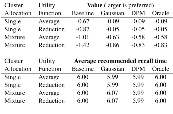
All three adaptive policies have larger (better) value than the static baseline policy in all cases. For

data generated from a single group, the Gaussian model is correct and produces value nearly identical to

the oracle policy. The DPM approach is also nearly identical to the oracle model in this case, showing that

little is lost in fitting a complex model in this simple case. When data are generated from the two-component

mixture model that includes non-compliers, the misspecified Gaussian model gives a policy with suboptimal

value and averaged recommended recall time that exceeds the six-month threshold. For the mixture model,

the DPM approach provides a substantial improvement over the Gaussian model.

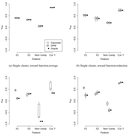
To gain further insight about the effects of model misspecification, Figure 1.4 plots the sampling

dis-tribution of the estimated policy weights αopt for each method, scenario and utility function. Both the

Gaussian and DPM methods giveαoptnear the oracle model for the single-group scenario. In this case, the

previous value ofY is the most important feature and thus the policy is to recommend shorter recall times

Table 1.1: Simulation study results comparing the baseline model with 6-month recommendation for all subjects, policy search methods based on Gaussian and Dirichlet process mixture (DPM) fits, and the oracle model which uses the true data-generating model to estimate the policy. The standard errors of the sample means are all less than 0.01.

Cluster Utility Value(larger is preferred) Allocation Function Baseline Gaussian DPM Oracle

Single Average -0.67 -0.09 -0.09 -0.09

Single Reduction -0.87 -0.05 -0.05 -0.05

Mixture Average -1.01 -0.63 -0.58 -0.58

Mixture Reduction -1.42 -0.86 -0.83 -0.83

Cluster Utility Average recommended recall time Allocation Function Baseline Gaussian DPM Oracle

Single Average 6.00 5.99 5.99 6.00

Single Reduction 6.00 5.99 5.99 6.00

Mixture Average 6.00 6.07 5.99 6.00

Mixture Reduction 6.00 6.07 5.99 6.00

data generated under the mixture model. For example, the importance of non-compliance is underestimated.

In contrast, the oracle model in Figure 1.4 (c) gives considerable weight to non-compliance to account for

non-compliers.

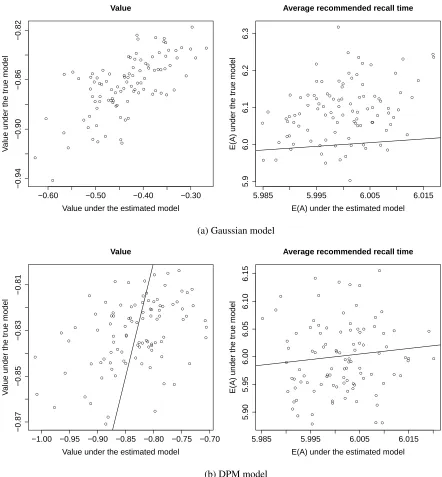
Model misspecification for the Gaussian case also affects the estimated value and average recommended

recall time of the policy. Figure 1.5 shows that the value is generally larger, thus overly optimistic when

evaluated using Monte Carlo simulations under the incorrectly fitted model than the true mixture model. In

practice, value must be estimated under the fitted model, which can be misleading if the model is incorrect.

The optimalαin (1.4) is a deterministic function of the model parametersgandS. Thus far, we have

been averaging over uncertainty ingandSto obtain an optimal policy. However, to quantify uncertainty in

the policy, we can inspect the posterior distribution ofαopt induced by the posterior distribution ofgand

S. To illustrate, we simulate 100 datasets generated from the two-component mixture model. We randomly

select posterior samples{g(j),S(j)_{;j = 1, . . . ,20}from allJ posterior draws produced by fitting the DPM}

model to the data. Given each selected posterior sample of model parameters, a posteriorαoptis estimated

using reduction utility function. We estimate 90% credible intervals ofαopt for each of the 100 simulated

Feature

αop

t −1.0 −0.5 0.0 0.5 1.0

X1 X2 Non−comp Cur Y

● ● ● ● ● Gaussian DPM Oracle

(a) Single cluster, reward function:average

Feature

αop

t −1.0 −0.5 0.0 0.5 1.0

X1 X2 Non−comp Cur Y

●

●

●

●

(b) Single cluster, reward function:reduction

Feature

αop

t −1.0 −0.5 0.0 0.5 1.0

X1 X2 Non−comp Cur Y

●

●

●

●

(c) Mixture clusters, reward function:average

Feature

αop

t −1.0 −0.5 0.0 0.5 1.0

X1 X2 Non−comp Cur Y

●

●

●

●

(d) Mixture clusters, reward function:reduction Figure 1.4: Estimated optimal feature weightsαopt for the simulation study. The boxplots for the Gaussian and

DPM methods show the estimatedαoptover the 100 simulated datasets; the solid points representαoptfor the Oracle

policy. The risk score is a linear combination the two baseline covariates (X1andX2), non-compliance (“Non-comp”;

● ● ● ● ● ● ● ● ● ● ● ● ● ● ● ● ● ● ● ● ● ● ● ● ● ● ● ● ● ● ● ● ● ● ● ● ● ● ● ● ● ● ● ● ● ● ● ● ● ● ● ● ● ● ● ● ● ● ● ● ● ● ● ● ● ● ● ● ● ● ● ● ● ● ● ● ● ● ● ● ● ● ● ● ● ● ● ● ● ● ● ● ● ● ● ● ● ● ● ●

−0.60 −0.50 −0.40 −0.30

−0.94

−0.90

−0.86

−0.82

Value

Value under the estimated model

V

alue under the tr

ue model ● ● ● ● ● ● ● ● ● ● ● ● ● ● ● ● ● ● ● ● ● ● ● ● ● ● ● ● ● ● ● ● ● ● ● ● ● ● ● ● ● ● ● ● ● ● ● ● ● ● ● ● ● ● ● ● ● ● ● ● ● ● ● ● ● ● ● ● ● ● ● ● ● ● ● ● ● ● ● ● ● ● ● ● ● ● ● ● ● ● ● ● ● ● ● ● ● ● ● ●

5.985 5.995 6.005 6.015

5.9

6.0

6.1

6.2

6.3

Average recommended recall time

E(A) under the estimated model

E(A) under the tr

ue model

(a) Gaussian model

● ● ● ● ● ● ● ● ● ● ● ● ● ● ● ● ● ● ● ● ● ● ● ● ● ● ● ● ● ● ● ● ● ● ● ● ● ● ● ● ● ● ● ● ● ● ● ● ● ● ● ● ● ● ● ● ● ● ● ● ● ● ● ● ● ● ● ● ● ● ● ● ● ● ● ● ● ● ● ● ● ● ● ● ● ● ● ● ● ● ● ● ● ● ● ● ● ● ●

−1.00 −0.95 −0.90 −0.85 −0.80 −0.75 −0.70

−0.87

−0.85

−0.83

−0.81

Value

Value under the estimated model

V

alue under the tr

ue model ● ● ● ● ● ● ● ● ● ● ● ● ● ● ● ● ● ● ● ● ● ● ● ● ● ● ● ● ● ● ● ● ● ● ● ● ● ● ● ● ● ● ● ● ● ● ● ● ● ● ● ● ● ● ● ● ● ● ● ● ● ● ● ● ● ● ● ● ● ● ● ● ● ● ● ● ● ● ● ● ● ● ● ● ● ● ● ● ● ● ● ● ● ● ● ● ● ● ●

5.985 5.995 6.005 6.015

5.90 5.95 6.00 6.05 6.10 6.15

Average recommended recall time

E(A) under the estimated model

E(A) under the tr

ue model

(b) DPM model

Figure 1.5: Value and average recommended recall time for the 100 datasets for the policy (via αopt) estimated

using the Gaussian model or DPM model for data generated from a two-component mixture model withn = 1,000

of the posterior draw ofgandSto obtain the posterior distribution of the optimal weightαopt. The coverage

rates of credible intervals for optimalα1,α2,α3,α4are 96%, 95%, 98%, 100% respectively, which indicates

that our estimated credible intervals are conservative and reliable.

1.7

Application: HealthPartners Data

1.7.1 Tailoring the BNP Model

The DPM model in (1.2) must be generalized to incorporate the complexities of the HP data. In the HP data,

the baseline covariate vectorXiincludes gender(Xi1), race(Xi2), standardized age(Xi3), diabetes status (Xi4), smoking status(Xi5)and commercial insurance indicator(Xi6). In the final model, we include

co-variates, such thatXit = [XTi , Yit−1,log(Ait),XTi log(Ait), Yit−1log(Ait)]T andZit= [XTi , Yit−1,log(δit), XT_i log(δit), Yit−1log(δit)]T. BecauseXi1,Xi2,Xi4,Xi5andXi6are binary, we introduce latent

continu-ous variablesX?_i to link the binary covariates to the DPM model,Xij =I(Xij? >0)forj= 1,2,4,5,6. For identification, we restrict the variance ofX_i?₁,X_i?₂,X_i?₄,X_i?₅,X_i?₆to be1. Also, with responses taking values

only in[0,1], we use the Tobit model (Tobin, 1958) to link the response to a continuous latent variableY?

whose support is(−∞,∞), and the observed variable is related to the continuous variable asY˜it = Y_it? if

0≤Y_it? ≤1,Y˜it= 0ifYit? <0and,Y˜it = 1ifYit? >1.

Then(X?T_i , Y_i?₀)T ∼Normal(θi0,Σ0)andYit?∼Normal(ZitTθi2, σ22).

After fitting the model to the HP data, diagnostic checks revealed evidence against the normality

assump-tion. Therefore, we use scale mixtures of normals to accommodate the heavier-tailed residual distributions,

such that

log(δit)|Θi,Xi, Yit−1, Ait ∼ Normal(XitTθi1, λit1σ21)

Y_it?|Θ_i,Xi, Yit−1, δit ∼ Normal(ZitTθi2, λit2σ22)

whereλit1 ∼Inv-Gamma(ν1/2, ν1/2),λit2∼Inv-Gamma(ν2/2, ν2/2). Also, as shown in Figure 1.1, there

such thatYitcan have excess probabilitypitonyit−1,

f(y|Yit−1 =yit−1) =pit1yit−1(y) + (1−pit)φ

?_(y|ZT

itθi2, λit2σ22)

wherepit = Φ(ZitTθi3),1yit−1(·)is the indicator function with a point mass atyit−1, andφ

?_(y|ZT

itθi2, λit2σ22)

is the density of the response variableY˜itin the Tobit model with meanZ_itTθi2and varianceλit2σ22, which

corresponds to a normal distribution for the latent response variable Y_it?. We assign the Dirichlet process

prior for the distribution of Θi = {θi0,θi1,θi2,θi3}. The hyperparameter values and MCMC details are

described in the supplemental material. The supplemental materials also include model comparisons and

goodness of fit diagnostics. We find that the DPM model described in this section with L = 10 mixture

components fits well and outperforms simpler methods. Therefore we use this model for the remainder of

the analysis.

1.7.2 Summarizing the Fitted Model

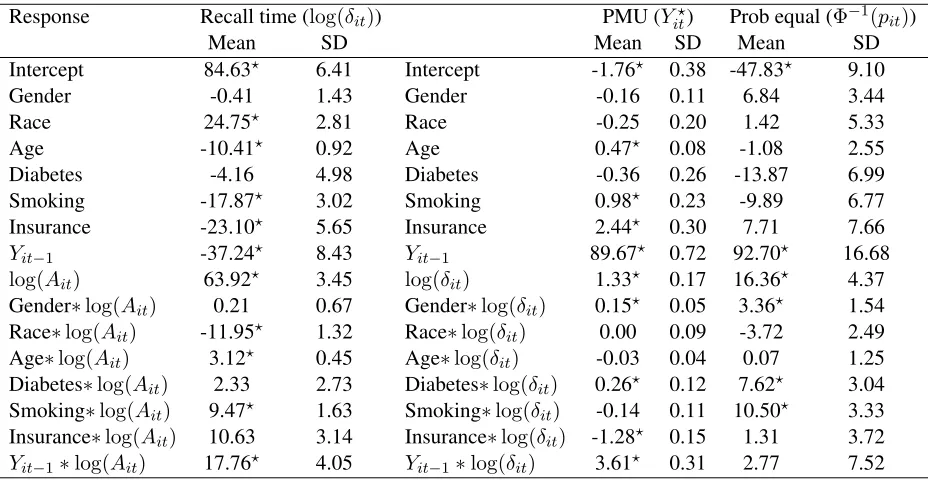
The posterior mean and standard deviation for average of(θ?T_1l ,θ₂?T_l,θ?T_3l )T weighted by the mixture

prob-abilitieswlforl = 1,2, . . . ,10are listed in Table 2.1. As expected, the recommended recall interval (Ait)

is the most important factor to determine the actual recall time (δit), and current disease status (Yit−1) is

the most important predictor to predict the disease status during next visit (Yit). The disease progression

between two visits is associated with the actual time between two visits, and the significantly positive

inter-action effect between current disease status and actual recall time onY_it? indicates that time effect is larger

for subjects with worse disease status. Also, most of the baseline covariates have significant effect on either

the actual recall time or disease progression.

1.7.3 Summarizing the Fitted Policy

While analyzing HP data, we use the policy in (1.3) witha1 = 3anda2 = 9, and a linear combination of

q = 4features representing standardized age (X3), diabetes status (X4 = 0for subjects without diabetes,

Table 1.2: The posterior mean×100 and standard deviation ×100for weighted average of random effects with

log(δit),Y_it?andΦ−1(pit)as responses, respectively. The posterior mean with “?” represents the corresponding95%

credible intervals that excludes zero.

Response Recall time (log(δit)) PMU (Yit?) Prob equal (Φ−1(pit))

Mean SD Mean SD Mean SD

Intercept 84.63? 6.41 Intercept -1.76? 0.38 -47.83? 9.10

Gender -0.41 1.43 Gender -0.16 0.11 6.84 3.44

Race 24.75? 2.81 Race -0.25 0.20 1.42 5.33

Age -10.41? 0.92 Age 0.47? 0.08 -1.08 2.55

Diabetes -4.16 4.98 Diabetes -0.36 0.26 -13.87 6.99 Smoking -17.87? 3.02 Smoking 0.98? 0.23 -9.89 6.77 Insurance -23.10? 5.65 Insurance 2.44? 0.30 7.71 7.66 Yit−1 -37.24? 8.43 Yit−1 89.67? 0.72 92.70? 16.68 log(Ait) 63.92? 3.45 log(δit) 1.33? 0.17 16.36? 4.37 Gender∗log(Ait) 0.21 0.67 Gender∗log(δit) 0.15? 0.05 3.36? 1.54 Race∗log(Ait) -11.95? 1.32 Race∗log(δit) 0.00 0.09 -3.72 2.49 Age∗log(Ait) 3.12? 0.45 Age∗log(δit) -0.03 0.04 0.07 1.25 Diabetes∗log(Ait) 2.33 2.73 Diabetes∗log(δit) 0.26? 0.12 7.62? 3.04 Smoking∗log(Ait) 9.47? 1.63 Smoking∗log(δit) -0.14 0.11 10.50? 3.33 Insurance∗log(Ait) 10.63 3.14 Insurance∗log(δit) -1.28? 0.15 1.31 3.72 Yit−1∗log(Ait) 17.76? 4.05 Yit−1∗log(δit) 3.61? 0.31 2.77 7.52

Yt−1). As the scale ofYt−1is much smaller than the other three features, we use10Yt−1in the risk score to

get more stable estimates of the feature weights:

Rt=X3α1+X4α2+ log(|δt−1−At−1|+ 1)α3+ 10Yt−1α4.

We have also tried replacing diabetes status (X4) with gender (X1) or smoking status (X5) in the construction

of the risk score, and this does not improve the valueV. We define the utility function as the reduction in

proportion of unhealthy sites in 5 years from baselineU(H) =Y0−YT60, whereYT60 is the response for a

subject in 5 years (60 months) since baseline visit (if no visit occurs at the exact time point, interpolation is

used to estimate the response value), and control the cost by constraining average recommended recall time

to beC(α) = 6months. We use5,000iterations in Gibbs sampling, and discard first3,000burn-in samples

to obtain2,000posterior samples by fitting the DPM model. We randomly draw 100 posterior samples ofg

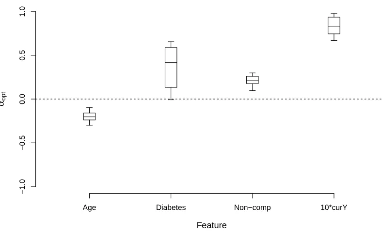
Figure 1.6 plots the posterior of αopt. The posterior mean weights for diabetes and non-compliance

are positive. This suggests that subjects with diabetes and non-compliers should be recommended to come

back to the dental clinic in a shorter time, reconfirming earlier findings on the link between diabetes and

PD (Mealey and Oates, 2006), and between recall compliance and medium to long-term PD therapy (Fenol

and Mathew, 2010). However, the posterior distribution of the weight for diabetes has a large variance.

The weight for the current disease status is significantly positive with high value, which indicates that the

current disease status is an important feature in determining recommendation decision, and the subject with

a higher proportion of diseased sites has a higher risk score and should be assigned shorter recall time. The

negative estimated weight for age indicates that younger subjects should have more frequent visits. It may

be that younger subjects are less stable, and so providing more visit opportunities to younger subjects might

improve population-level benefits.

We also estimate one final optimal policyαoptaveraging over uncertainty ingandS, which gives the

risk score functionRt=−0.17X3+ 0.50X4+ 0.22 log(|δt−1−At−1|+ 1) + 8.2Yt−1with a threshold1.06.

This risk score function suggests that subjects with diabetes tend to have higher risk than subjects without

diabetes, and the disease status is the most important feature that decides the recommended recall time. For

example, a subject with diabetes, average age (X3 = 0) and perfect compliance (δt−1 =At−1) should come

back in 3 months if his/her proportion of unhealthy sites is higher than6.8%. A subject without diabetes and

with average age and perfect compliance should come back in 3 months if his/her proportion of unhealthy

sites is higher than12.9%.

The value corresponding to the estimated optimal policy is V(αopt) = −0.0102with standard error

0.0002, which is estimated by Monte Carlo Simulation with100,000simulated subjects. Compared to the

‘baseline’ policy which recommendsAt= 6months between visits for all subjects andtand with estimated

V = −0.0170 with standard error 0.00018, the utility value averaging over the entire distribution of H increases by about40%. This is a substantial improvement, especially when the improvement of expected

value is multiplied by the number of people in the population.

Furthermore, to explore the effects of choosing a linear function of the subject characteristics and current

Feature αop

t

Age Diabetes Non−comp 10*curY

−1.0

−0.5

0.0

0.5

1.0

Figure 1.6: Posterior distribution (5th, 25th, 50th, 75th, 95th percentiles) of optimal feature weightsαoptfor the HP

most important feature) in constructing the risk score. The estimated risk score isRt=−0.38X3+0.55X4+

0.25 log(|δt−1−At−1|+ 1) + 3.2Yt−1+ 63Yt2−1, with the value−0.0101, which is very close to the value

−0.0102 corresponding to the optimal policy under the class of policies with only linear function of the

features. Hence, we advocate using only linear features for this dataset.

1.8

Conclusions

Motivated to address the shortcomings of the classic 6-month recall interval in periodontal treatment

alloca-tions, we present a policy-optimized recommendation engine using BNP that exhibits superior performance

compared to alternatives. We show using simulation studies that the proposed method provides a valid

poste-rior inference, and can reliably identify the optimal policy. Applying the method to the HP data, we find that

the optimal policy recommends more frequent visits for young, unhealthy non-compliers, and that following

this policy could lead to a substantial reduction in PD.

A number of computerized periodontal risk assessment tools are currently available (Page et al., 2003;

Persson et al., 2003). For example, the Cigna PD self-assessment tool available at https://www.

cigna.com/individuals-families/health-wellness/gum-disease-assessment

considers subject-specific inputs through a questionnaire, and combines information from the PD fact

sheet of the American Academy of Periodontology to calculate a simple ordinal risk score (low, low to moderate, moderate, or high), without any guidance towards recall intervals. There exists a number of

popular chairside software in practice-based dentistry (such as Patterson’s Eaglesoft®) that record and

display data. Supplementing these tools with an evidence-based recommendation system for periodontal

recalls would aid practitioners.

A limitation of our analysis is that we use periodontal pocket depth (PPD) rather than the most reliable

endpoint (AAP, 2005) clinical attachment level (CAL). Site-level full mouth CAL assessment in a

practice-based observational data setting like ours is time-consuming and technically demanding (Michalowicz et al.,

2013). For example, in the HP dataset, CAL is computed only for the mid-buccal and mid-lingual sites,

whereas, the PPD is calculated for all 6 sites on each tooth (if that tooth is present). Also, since CAL is

1992; Hill et al., 2006). Hence, we considered thresholded site-level PPD in addition to missing tooth to

compute the proportion subject-level endpoints. The missing tooth in our analysis is assumed missing due to

past incidence of PD, and the error generated from the apparent misclassification of the missingness source

(such as, tooth falling out due to mechanical injury) is usually negligible while analyzing large observational

databases. Should CAL and PPD measures become available for all sites (in other databases), our framework

can readily incorporate this information. In addition, to reduce computational burden, our present policy

only considers recall intervals of 3 and 9 months. Our method can be easily extended to more than two

possible actions by adding thresholds to the risk score. Computationally, estimating an optimal threshold

parameter should be similar to estimating a feature weight. Therefore, the proposed decision framework is

quite general, and can be adapted to the specific needs of the practitioner.

To the best of our knowledge, this is thefirst studyto cast the century-old debate on periodontal recall intervals into a DTR stochastic framework. Our recommendation tool is derived from a specific US

mid-western population, and its generalizability is not evaluated here. Longitudinal PD databases from other

practice-based settings (such as Kaiser Permanente®) may be combined with the current HP database to

refine findings. Furthermore, our present recall engine is geared exclusively towards PD assessment and

do not include (dental) caries risk, although evidence suggest that they may occur simultaneously (Mattila

Chapter 2

A Spatiotemporal Recommendation Engine

for Malaria Control

2.1

Introduction

Malaria is a vector-borne infectious disease affecting a large population worldwide, especially in tropical

and subtropical regions (Guerra et al., 2008). It is estimated that there were 216 million cases of malaria

re-sulting in 445,000 deaths globally in 2016 (WHO, 2017), and thus it remains a major public health problem.

Effective malaria interventions have been developed, including insecticide-treated mosquito nets (ITNs)

(Lengeler, 1998), indoor residual spraying (IRS) (Pluess et al., 2010), and Artemisinin-based combination

therapy (ACT) (Eastman and Fidock, 2009). However, these interventions are too costly to be given to

every-one in need. The malaria research community has made great strides in mapping disease prevalence (Bhatt

et al., 2015, 2017; Kang et al., 2018; Hay et al., 2009), modeling its transmission (Griffin et al., 2010, 2014,

2016; Bhadra et al., 2011), developing and testing effective interventions (Okell et al., 2014; Stuckey et al.,

2014; Parham and Hughes, 2015; Walker et al., 2016), and implementing these interventions in practice. We

propose to build on this work to develop a real-time recommendation engine (RE) for precision interventions

to help policy-makers decide how to best allocate limited resources.