Biomimicry of Learning Complex Movements by Coordination of Simple Least-Effort Parts.

(1)

ABSTRACT

REININGER, TAYLOR JACOB. Biomimicry of Learning Complex Movements by Coordination of Simple Least-Effort Parts. (Under the direction of Dr. Larry Silverberg).

This thesis explores the introduction of a biomimicry technique in which simple, least effort

movements are coordinated together to create highly complex and useful movements

mimicking those found in nature. The method described in this paper provides an intuitive

approach for creating high efficiency movements while achieving complex goals, thus

mimicking the learning process.

The approach breaks down the movements of a physical system into the most elementary

components and parameterizes the movements to allow for manipulation. By optimizing the

movements, least effort solutions can be obtained. Higher levels of complexity can be created

by coordinating multiple movements of lower complexity levels.

To demonstrate the suggested approach, a specific example is used. A two linkage simulation

is created in MATLAB® to mimic a human arm. The human arm is taught to produce

movements of increasing complexity, while striving for least effort solutions. Four levels of

complexity are observed to illustrate the method for constructing movements of increasing

complexity. To further analyze the results of this experiment, a comparison of gaits is created

to observe the methodology of path selection and further verify the accuracy of the obtained

results.

It is found that this method provides a solution for creating a variety of movements of

varying complexity. It is also discovered that the movements created by this method appear

life-like and are aesthetically pleasing, and tend to behave similarly to the systems they are

intended to mimic. Furthermore, it is observed that gait selection through this method is

(2)

(3)

Biomimicry of Learning Complex Movements by Coordination of Simple Least-Effort Parts

by

Taylor Jacob Reininger

A Thesis submitted to the Graduate Faculty of North Carolina State University

in partial fulfillment of the requirements for the degree of

Master of Science

Mechanical Engineering

Raleigh, North Carolina

2016

APPROVED BY:

_______________________________ _______________________________

Dr. Larry Silverberg Dr. Chih-Hao Chang

Committee Chair

_______________________________ _______________________________

(4)

ii DEDICATION

This thesis is dedicated to my two loving parents, Ken and Jacquie, whose love, support, and

(5)

iii BIOGRAPHY

Taylor was born in Syracuse, New York to parents Ken and Jacquie Reininger. At age 3,

Taylor’s family moved to Asheboro, North Carolina where his parents began home schooling

him, and continued to do so until he graduated high school. Taylor has always had a passion

for sports, science, and the NC State Wolfpack! During his time at NC State, Taylor rushed

the court multiple times at rivalry basketball games, was voted Faculty Senior Scholar by the

(6)

iv ACKNOWLEDGMENTS

First, I would like to thank my incredible parents for giving me so many opportunities to

succeed and supporting me every step of the way. It is to their emphasis on personal

excellence and taking pride in one’s work that I attribute my successes.

I would like to thank Dr. Larry Silverberg for encouraging me to attend graduate school and

for being my mentor for so many years, and agreeing to serve as my committee chair. I

would also like to thank Dr. Chau Tran, Dr. Chih-Hao Chang, and Dr. Edgar Lobaton for

helping me find my path over the last 6 years and for serving as committee members for this

thesis.

I would also like to thank Thomas Powers, Chris Yoder and Dr. James Kribs, without whom

I would not have made it through grad school, and for the many brainstorming sessions over

the years.

I also want to thank my girlfriend, Beth May, who was always there for me through all the

ups and downs of one of the hardest, and most rewarding, times of my life.

(7)

v TABLE OF CONTENTS

LIST OF TABLES ... vii

LIST OF FIGURES ... viii

DEFINITIONS ... ix

1. Introduction ...1

1.1. Overview ...1

1.2. Topic ...1

1.3. Literature ...1

2. Method ...2

2.1. Overview ...2

2.2. Elementary Movements ...2

2.3. Parameterization...3

2.4. Optimization ...3

2.5. Control Theory ...3

2.6. Coordination ...5

2.6.1. Level 1 ...5

2.6.2. Level 2 ...6

2.6.3. Higher Levels ...8

2.7. Defining Success ...8

3. Results ...9

3.1. Overview ...9

3.2. Incremental Learning ... 10

3.2.1. Level 1 ... 10

3.2.2. Level 2 ... 10

3.2.3. Level 3 ... 10

3.2.4. Level 4 ... 13

3.2.5. Comparison ... 14

4. Conclusion... 17

4.1. Incremental Learning ... 17

4.2. Gaits ... 17

4.3. Future Work ... 18

4.3.1. New Limbs ... 18

4.3.2. Increased Degrees-of-Freedom ... 18

4.3.3. Three Dimensions ... 18

4.3.4. Higher Motion Complexity ... 19

REFERENCES... 20

APPENDICES ... 21

Appendix A : Parameterization ... 22

Gauss Error Function ... 22

Appendix B : Optimization ... 24

Cost Function ... 24

Steepest Descent ... 26

Appendix C : Control ... 27

(8)

(9)

vii LIST OF TABLES

Table 1: Path 1 & 2 Cost Comparison, Five Second Completion Time ... 15

Table 2: Path 1 & 2 Cost Comparison, Ten Second Completion Time ... 15

Table 3: Path 1 & 2 Comparison, Many Completion Times ... 16

Table 4: Level 1, Modes ... 23

Table 5: Level 2, Movements ... 24

Table 6: Cost Function ... 26

Table 7: Controller Terminology ... 27

Table 8: Tracking and Regulation ... 27

Table 9: Shifting and Scaling Design Variables ... 29

Table 10: State Variables ... 31

Table 11: Linkage Positions at Ends ... 31

Table 12: Linkage Velocities at Ends... 32

Table 13: Joint Constraints ... 32

Table 14: Linkage Joint Relative Position and Velocity ... 32

Table 15: Reaction Forces on Linkages ... 33

Table 16: Reaction Moments ... 33

Table 17: State Equations ... 33

(10)

viii LIST OF FIGURES

Figure 1: Two-Linkage Arm ...2

Figure 2: Loose Controller Gains ...4

Figure 3: Tight Controller Gains ...4

Figure 4: Increasing Complexity ...5

Figure 5: Gaussian Error Function Plot ...6

Figure 6: Mode 1 Movement, Rotation ...7

Figure 7: Mode 2 Movement, Extension ...7

Figure 8: Mode 1 Theta vs. Time ...7

Figure 9: Mode 2 Theta vs. Time ...7

Figure 10: Free Body Diagram of Linkages ...9

Figure 11: Goal Level 3, Movement 1 ... 11

Figure 12: Time Lapse Level 3, Movement 1 ... 11

Figure 19: Level 4 Start Position and Goal ... 13

Figure 20: Time Lapse Level 4 Path 1 ... 14

Figure 21: Time Lapse Level 4 Path 2 ... 14

Figure 22: Time Lapse of Path 1 at Ten Seconds ... 15

Figure 23: Time Lapse of Path 2 at Ten Seconds ... 15

Figure 24: Path 1 & 2 at Various Times ... 16

Figure 25: Gauss Error Function with Varying Magnitude ... 22

Figure 26: Gauss Error Function with Varying Smoothness ... 22

Figure 27: Gauss Error Function with Varying Time ... 23

Figure 28: Error Function Scaled and Shifted ... 24

Figure 29: Level 3 Movement 1 ... 30

Figure 30: Level 3 Movement 2 ... 30

(11)

ix DEFINITIONS

Name Definition

𝑘 Motion Sharpness

𝑇 Motion Time

𝑀 Motion Magnitude

Linkages The members that make up the simulation

End Point The location of the free end of the second linkage

Initial Position The position of the linkages at the beginning of a movement Final Position The position of the linkages at the completion of a movement Completion Time The amount of time a simulation is given to complete a movement End Goal The assignment for the end point to reach by the completion time Level A hierarchy used to designate the complexity of movements during

the learning process

Path The total prescribed motion regardless of which level it falls in Simple Movement A relative term denoting parts to be coordinated into complex

movements, the lower of two Levels

Complex Movement A relative term for the result of coordinating two simple movements, the higher of two Levels

(12)

1

1. Introduction

1.1. Overview

Biomimicry has long been a source of innovation for engineering applications. Many

engineering challenges have been solved by drawing from the nearly four billion years of

evolution and problem solving of biology. Applications include mimicking materials,

motions (biomechanics), and even natural selection itself [1,2]. This paper studies the

concept of motion learning as a biomimicry technique for creating complex movements by

coordinating a number of simple movements together.

1.2. Topic

The natural movement of articulating members can be complex, as well as beautiful. The

necessity for complex motion is evident in daily life, though the creation of such motion is

difficult to construct. As humans, these motions are learned from a young age, starting with

simple motions, like extending a leg away from the body or grabbing an object. As simple

motions are mastered, more complex movements are developed, like crawling or waving.

Each movement is learned by recalling past movements and is iteratively improved upon for

future uses. The concept of using simple parts to construct more complex parts is a common

theme in biology and society. This topic builds upon research by Passino which outlines

cascaded path planning with increasing complexity and other methods for reducing effort [3].

1.3. Literature

There are many current uses for this type of technology that span a wide range of

applications. Boston Dynamics has created a number of robots that mimic biology. Boston

Dynamics’ Cheetah robot mimics the running motion of a four legged animal and the Atlas

robot mimics a human with bipedal walking, lifting objects, and manipulating the

environment around it [4]. Johns Hopkins Applied Physics Laboratory is currently

developing human arm prosthetics that closely emulate natural movement with intent to

enhanced user compatibility in their Revolutionizing Prosthetics program [5]. ABB

Automation makes robotic arms for manufacturing that are capable of highly complex

motion [6]. All of these industries draw from biomechanics and could benefit from the

(13)

2

2. Method

2.1. Overview

This paper explores the method of training robotic motion through the use of coordination.

The concept is to construct any number of complex movements with a combination of simple

movements that have already been learned. It is theorized that this will provide intuitive,

efficient, and aesthetically pleasing results, much like those found in nature. This method

may prove to allow for highly sophisticated movements, such as those that require both range

and precision, since simple motions are optimized individually and cascaded together to

create the required complex motions. It is also theorized that many levels of complexity will

exist, ranging from elementary to highly complex.

2.2. Elementary Movements

To begin this process, it is first necessary to identify the most elementary of movements. The

most elementary movements a system is capable of will vary in quantity and nature

depending on the system at hand. To illustrate this concept, it is helpful to use an example.

Take the case of a two linkage system, representing the upper and lower components of a

human arm with gravity acting in the negative y-direction, as is customary. The first linkage

is pinned to the origin at one end and to the second linkage at the other end, thus creating a

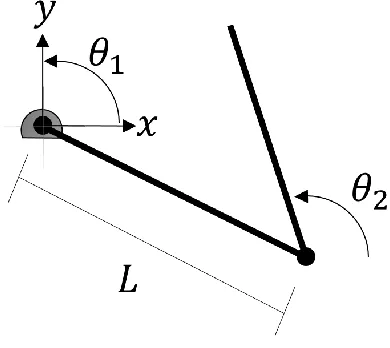
chain of length two. Figure 1 shows the components of the two linkage arm example.

Figure 1: Two-Linkage Arm

The system should be controllable in order to produce motion, so consider the case in which

(14)

3 at each joint to produce rotation in the linkages. Thus by the method outlined in this topic,

there are two elementary movements the system is capable of. The first involves only the

motor at the origin, or the “shoulder joint”. The second elementary movement involves only

the motor where the linkages are connected, or the elbow joint. Both elementary movements

can move only once and in only one direction.

2.3. Parameterization

Once the most elementary movements of the system are identified, they must be

parameterized. Values must be defined which will influence the movement so that it can

easily be modified. It is necessary to identify parameters in both time and space, though it is

possible to decouple the two, thus reducing the complexity of the movement. For the

example with the two-linkage arm, three parameters are identified for each elementary

movement. The three parameters are: how much the linkage moves, when the movement

occurs, and how long the movement takes. These parameters allow for simple manipulation

of the elementary movement, and are crucial building blocks for subsequent steps. More

information on the parameterization process for this research can be found in Appendix A.

2.4. Optimization

From previous research, it is clear that biological processes strive to minimize effort

[3][7][8]. Everything from crowd patterns to communication methods include some level of

least-effort solutions. It is, therefore, beneficial to attempt to minimize effort in the desired

movements to further mimic the methods of biological learning. This can easily be done

through the use of optimization techniques. Optimization of any movement requires a

balance between achieving the end goal while exerting the least amount of effort possible.

The optimization function adjusts the variables used to parameterize the elementary

movements to create a desirable solution. The manipulation of the movement through

optimization serves to automate the process of finding the least effort solutions. More

information on the optimization process for this research can be found in Appendix B.

2.5. Control Theory

In order to create motion in the system, a path is prescribed to each linkage as a function of

time. The controller manipulates the motors in an attempt to follow the prescribed path. For

this simulation, a Linear Quadratic Regulator is selected as the control method for the

(15)

4 [9]. The Linear Quadratic Regulator used during this experiment implemented tracking and

regulation control to manipulate the linkages [10]. This method divides the control into two

distinct tasks. The tracking portion of the controller uses the moment of inertia of the

linkages and the required angular acceleration to calculate the moment necessary to induce

the desired motion. This portion of the controller requires previous knowledge of the system

parameters in order to calculate the moment of inertia. The tracking component does not

account for disturbances resulting from gravity or other external forces and moments, such as

those imposed by the other linkage. The regulation portion of the controller is tasked with

maintaining the desired path despite external disturbances to the system. This functions much

like a classic Proportional-Derivative controller in that it regulates the angular position and

angular velocity to match the desired position and velocity, respectively. This task also

requires sensors to determine the actual position of the linkages, something that is simplified

by a simulation. The regulation control also requires gains for the sensitivity to position and

velocity error, and tuning of these gains is necessary to create a stable and functional

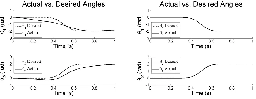
controller. Figure 2 and Figure 3 show a comparison of controller behavior with different

gains.

Figure 2: Loose Controller Gains Figure 3: Tight Controller Gains

Notice that in Figure 3, the desired path and actual path are nearly indistinguishable. For the

remainder of the paper, the desired paths will not be shown, as the controller is tuned to

follow the prescribed path. The effort of the motion is determined from the power consumed

by the motors during the movement. Therefore, the effort of the movement is directly

affected by the prescribed path. More information on the control process for this research can

(16)

5

2.6. Coordination

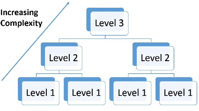
After optimizing the elementary movements, it is possible to construct movements of higher

complexity. To construct a movement of higher complexity, two simpler movements are

combined. At the lowest level of complexity, the simple movements are the elementary

movements. The process of combining two elementary movements to create a complex

movement is called coordination. For the two linkage example, one elementary movement is

bending the arm at the elbow and the other is rotating the arm at the shoulder. By

coordinating these two simple movements, a complex movement is created which involves

both rotating the shoulder and bending the elbow. The resultant movement is then

parameterized, and the process can continue to create increasingly complex movements.

Figure 4 shows simple movements being coordinated to create more complex movements at

two consecutive levels.

Figure 4: Increasing Complexity

It is possible to continue this approach indefinitely, though it becomes clear that highly

sophisticated and lifelike movements are achievable after only three or four levels of

coordination.

2.6.1. Level 1

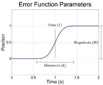
In order to create motion, a path must be prescribed. The Gaussian Error Function (erf) is

ideal for creating a path that both starts and ends at rest [11]. For the sake of simplifying the

simulation, all motions in this study have been limited to those that meet this criteria, and do

(17)

6 denoted as the completion time. Another benefit of the Gaussian Error Function is that it can

be easily manipulated in three ways by modifying the variables in the function. A sample

Gaussian Error Function (erf) equation can be seen in Equation (1).

𝐺𝐸𝐹(𝑡) = M

2erf⁡(𝑘(𝑡 − T)) (1)

Where 𝑡 is time, 𝑀 is the magnitude of the motion, 𝑘 is the sharpness of the transition, and 𝑇

is the moment in time that the motion is centered about. 𝐺𝐸𝐹 is a path as a function of time

that both starts and ends at rest. A sample Gaussian Error Function plot is shown below in

Figure 5.

Figure 5: Gaussian Error Function Plot

With control over the magnitude of the motion, sharpness of the motion, and time at which

the motion occurs, the linkage can be made to perform a variety of elementary movements.

2.6.2. Level 2

Level 2 movements are created by coordinating two Level 1 movements. For this

coordination, Level 1 movements are considered simple and Level 2 movements are

considered complex. When selecting the Level 2 movements, it is important to plan ahead

(18)

7 the Level 2 movements created. To achieve this, orthogonal movements can be created to

encompass the largest range of motion with the least number of coordinations. For the

example of the two linkage arm, the selected Level 2 movements are extension or retraction

of the end point in the radial direction (r) and rotation of the arm in the angular direction (𝜃),

thus creating polar coordinates for the end point. For the duration of this paper, these Level 2

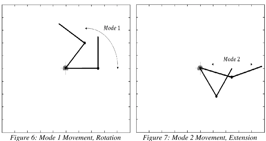
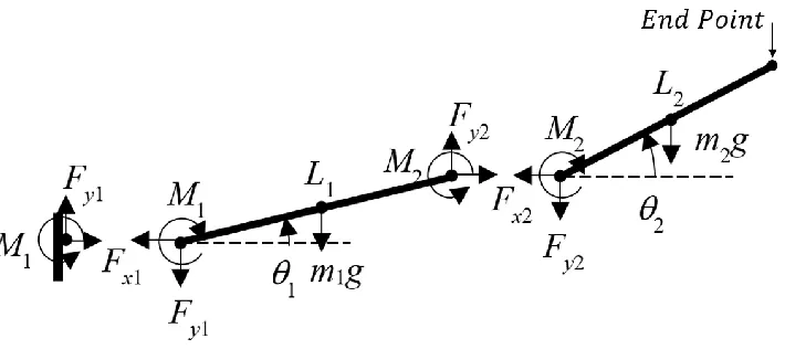
movements are called modes since they correlate to orthogonal movements. In the

simulation, prescribing the first mode will create the motion in Figure 6, and prescribing the

second mode will create the motion in Figure 7.

Figure 6: Mode 1 Movement, Rotation Figure 7: Mode 2 Movement, Extension

Figure 8 shows a path prescribed by the first mode and Figure 9 shows a path prescribed by

the second mode.

(19)

8 These movements are complex relative to the elementary movements in Level 1, but are still

quite basic.

2.6.3. Higher Levels

The method for coordinating higher levels is similar to that used in creating Level 2

movements in that the two simple movements are combined to create one complex

movement. The biggest difference higher levels have from lower levels is that there are a

much greater number of possible movements. For example, in the two linkage arm case,

Level 2 movements can be characterized into Mode 1 and Mode 2, thus covering the entire

capability of the system at Level 2. It is much more difficult to use the same approach on

Level 3, because the capability of the system is much greater. Attempting to categorize all

possible movements becomes increasingly more difficult as the levels progress, thus making

the approach undesirable. Therefore, it is decided that movements at Level 3 and higher

should be selected based on the specific needs of the user, and with the end goal in mind,

rather than attempting to encompass the entire realm of possible movements. More

information on the coordination process for this research can be found in Appendix D.

2.7. Defining Success

In order to create the desired movements, it is first important to define the characteristics of

success. As defined by the researcher, the ultimate goal of any motion is to touch the end

point to a desired position in Cartesian coordinates. This goal serves many purposes since it

is relatively precise and pertains to many industrial applications. It is interesting to note that a

large portion of the motions carried out by living organisms can be considered a combination

of simple end point assignments. Another key element to a successful motion is to consume

the least amount of effort possible. By conserving effort, the motion becomes less costly on

the system in terms of wear and fuel usage [12]. In addition to achieving the desired end goal

and conserving effort, other markers of success include completing the motion in a timely

manner and re-establishing rest at the final position. For this reason, every simulation has a

completion time in which the motion is required to be completed, and the linkages are to

return to rest.

It is important to note that in a two link system, any end point assignment will produce, at

(20)

9 the final configuration contains an infinite number of possibilities. Thus, it is the goal of this

research to study the path with which success is achieved rather than the final position.

3. Results

3.1. Overview

The results of this research are based on the two linkage arm example. The two linkage case

is simple to model and intuitive to observe, yet elaborate enough to construct highly complex

movements. A two linkage arm is simulated to mimic the mass and dimensions of the arm of

a human arm. For this experiment, the free end of the second linkage is considered the point

of interest, as this would be the location of a hand. All tasks involving an end goal will

impose position requirements on the free end of the second linkage, which from now on will

be referred to as the end point. A free-body diagram of the two linkage arm is shown in

Figure 10.

Figure 10: Free Body Diagram of Linkages

In order to make the system controllable, a motor is simulated at each pin and is used to

modify the angle of the respective linkage. The angle at 𝜃₁ is controlled by applying a

shoulder-like point moment at the origin. The angle at 𝜃₂ is controlled by applying an

elbow-like point moment at the joint between linkage one and linkage two. To simplify the

simulation, no limitation in the range of motion of the two joints is applied. More

(21)

10

3.2. Incremental Learning

3.2.1. Level 1

Level 1 movements are constructed with the same method outlined in Section 2.6.1. Gaussian

Error Functions are used to change the position of a single member. For the example of the

two linkage arm simulation, these paths correlate to the angle of each linkage in radians, as a

function of time.

3.2.2. Level 2

Level 2 movements are constructed with the same method outlined in Section 2.6.2. For the

example of the two linkage arm simulation, the two modes consist of moving the end point in

and out from the shoulder radially, and rotating the entire system as one about the shoulder.

These two modes provide a strong foundation for creating movements of higher complexity.

3.2.3. Level 3

The third level of complexity involves coordinating two Level 2 movements together to

create a Level 3 movement. This is the same process as creating Level 2 movements from

Level 1 movements, except there are no longer obvious choices for which movements to

create. Level 3 movements are more sophisticated, thus allowing more useful motions to be

created, so it is more important to create useful Level 3 movements than to create every

conceivable movement at this level. For this research, several tasks are constructed that

humans use every day, including bringing the end point in close to the body or raising it

above the shoulder. A library of the movements achievable at Level 3 can be created; four

distinct Level 3 movements are created for this example.

The first movement starts from an initial position which holds the arm out straight at -45

degrees from the positive x-axis. The movement then brings the end point up and in towards

the shoulder by using both Mode 1 and Mode 2. Figure 11 shows the initial position and the

end goal of this movement, denoted by a red “x”, and Figure 12 shows the time lapse of the

(22)

11

Figure 11: Goal Level 3, Movement 1 Figure 12: Time Lapse Level 3, Movement 1

The second movement starts at a similar position to the one that movement 1 ended at. The

end point begins near the shoulder before lifting out and above the origin to hold the arm

straight out at +45 degrees from the positive x-axis. Figure 13 shows the initial position and

end goal of this movement, and Figure 14 shows the time lapse of the least effort motion

prescribed by this movement.

The third movement starts with the initial position straight out from the shoulder at -45

degrees from the positive x-axis, just like the first movement. The movement then places the

end point level with the shoulder with the arm straight out on the positive x-axis. Figure 15

shows the initial position and end goal of this movement and Figure 16 shows the time lapse

(23)

12

It is interesting to note that the chosen path for the third movement almost completely

neglects to utilize Mode 2, since the end point begins at the desired radius from the shoulder.

The forth movement initial position consists of the arm held straight out on the positive

x-axis, similar to where the third movement ended. The movement then places the end point

out and away from the origin to hold the arm straight out at +45 degrees from the positive

x-axis. This is the same end point as prescribed in the second movement. Figure 17 shows the

initial position and end goal of this movement and Figure 18 shows the time lapse of the least

effort motion prescribed by this movement.

It is, again, interesting to note that this movement neglects to utilize much of Mode 2, since

the initial radius begins near the desired radius of the end point.

These movements have been chosen to create a specific set of tasks in Level 4 as described in

(24)

13 3.2.4. Level 4

Level 4 movements continue the trend by combining two Level 3 movements to create an

even higher level of complexity. At this point, there is very little the arm is incapable of

doing, so it is possible to construct very intuitive movements. For this reason, this level

allows for the comparison of gaits which seek to identify the advantages and disadvantages

of a particular path, even if the same end goal is achieved [13]. The study of gaits explores

the manner in which the goal is achieved, making it a useful topic of exploration. The use of

gaits to compare movements provides further insight into why biomimicry is such a useful

method for creating complex movements.

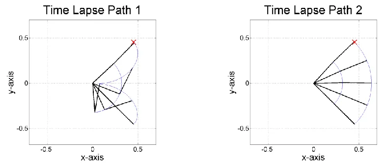
To do this, two identical goals are achieved through two different means. The goal is to lift

the arm from a straight out position at -45 degrees to a straight out position at +45 degrees

from the positive x-axis with a five second completion time. Path 1 brings the end point in

towards the shoulder to reduce gravitational forces before moving it out and upward to the

end goal. Path 2 rotates the end point out horizontally, without bringing the end point in

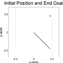
towards the shoulder, before continuing upward to the end goal. Figure 19 shows the initial

position and end goal for both cases.

(25)

14 The movement for Path 1 combines the movements created at Level 3 shown in Figure 12

and Figure 14. The initial position of the movement is straight out, at -45 degrees from the

positive x-axis. The movement then brings the end point in towards the shoulder as done in

Level 3, movement 1. The movement then continues to place the end point out and above the

origin to straight out, at +45 degrees from the positive x-axis.

The path taken for Path 2 combines the movements created at Level 3 shown in Figure 16

and Figure 18. The initial position of the movement is straight out, at -45 degrees from the

positive x-axis. The movement then places the end point level to the shoulder with the arm

straight out on the positive x-axis, as done in Level 3, movement 3. The movement then

continues to place the end point out and away from the origin to hold the arm straight out, at

+45 degrees from the positive x-axis. This is the same end point as prescribed by the Path 1

movement.

Figure 20 shows the time lapse of the motion prescribed by Path 1, and Figure 21 shows the

time lapse of the motion prescribed by Path 2.

Figure 20: Time Lapse Level 4 Path 1 Figure 21: Time Lapse Level 4 Path 2

It is interesting to note that Path 2 is considerably more direct than Path 1, while both achieve

the same outcome.

3.2.5. Comparison

By observing the two gaits, a comparison of the paths can be made. In this comparison, all

Level 3 movements have one second completion times and all Level 4 movements have five

(26)

15

Table 1: Path 1 & 2 Cost Comparison, Five Second Completion Time

Path 1 Path 2

Level 3 Movement 1 1352.41 323.08

Level 3 Movement 2 892.34 246.59

Level 4 Movement 931.76 381.97

It is clear that both the Level 3 and Level 4 movements are less costly in Path 2. This is not

surprising because the path is quite direct. Through observation of the human body, however,

it is evident that sometimes Path 1 is chosen over Path 2. Intuition suggests that the choice of

paths may be dependent on how fast the movement is to be executed. To investigate the

effect that completion time has on path selection, the same Level 3 movements are used to

create similar Level 4 movements, but with ten second completion times instead of five. The

time lapse for Path 1 can be seen in Figure 22, and the time lapse for Path 2 can be seen in

Figure 23.

Figure 22: Time Lapse of Path 1 at Ten Seconds

Figure 23: Time Lapse of Path 2 at Ten Seconds

Table 2 shows the design variables and costs of the two paths at ten seconds.

Table 2: Path 1 & 2 Cost Comparison, Ten Second Completion Time

Path 1 Path 2 456.15 829.28

It is seen that with a ten second completion time, Path 1 proves to be the least costly solution.

This finding makes it clear that the chosen path depends greatly on the total time of the

(27)

16 performed ranging from 1-15 seconds. The results from the comparisons are summarized in

Table 3.

Table 3: Path 1 & 2 Cost Comparison, Many Completion Times

Time Path 1 Path 2

1.00 5530.36 1223.44 2.00 2366.81 471.76 3.00 1464.72 326.25

5.00 931.76 381.97

7.75 572.27 575.61

10.00 456.15 829.28

15.00 698.78 1312.35

The data from Table 3 is plotted in Figure 24.

Figure 24: Path 1 & 2 at Various Times

It can be seen that Path 2 has a distinct advantage over Path 1 when the time of the

movement is relatively short. This is due to the fact that the movement is direct, thus

reducing the amount of acceleration required to complete the task within the completion

time. It can also be seen that Path 1 has a distinct advantage over Path 2 when the completion

(28)

17 closer to the shoulder, thus reducing the moment applied to the arm by gravitational

acceleration.

It is also interesting to note that the cost increases rapidly for both paths as the completion

time approaches zero. This can be attributed to the acceleration required to produce the

desired results in a very short time span. It is also interesting to note that the cost of both

paths increases steadily as the completion time increases beyond ten seconds. This can be

attributed to the greater time over which the motors must overcome gravity to keep the arm

up.

4. Conclusion

4.1. Incremental Learning

This study provides an in-depth analysis of a method for training advanced locomotive skills

through incremental learning. It is concluded that the method outlined in this paper can be a

useful technique for methodically creating complex movements. By providing least effort

solutions through the method of optimized coordination, biomimicry is achieved. It is also

clear from the results that predictable and intuitive solutions can be obtained. These results

closely mimic the behavior of natural movement by humans and other animals, thus

providing possible uses in prosthetics or other industries in which human interaction with the

device may be required. It can be concluded that part based learning with increasing

complexity can create efficient, reliable solutions in various applications of path planning.

Furthermore, incremental learning may provide advantages over other methods of path

planning with respect to computational power and memory storage requirements. It should

also be noted that this concept could be extrapolated to other applications that involve motion

planning such as walking, running, or throwing.

4.2. Gaits

The study of gaits in this topic serves to provide insight into decision making in motion

planning based on the given constraints in time and space. The example results confirm that

reducing the effect of gravitational acceleration is superior over long periods of time while

increasing the directness of the movement is superior over short periods of time. The results

found that both paths examined produce similar costs at the completion time of 7.75 seconds.

(29)

18 and greater than 10 seconds, begin penalizing the motion for power consumption

requirements. This serves to provide further insight into completion time selections for real

human motion, and builds confidence in the results.

It is useful to compare the results of the simulation with those of humans, since the

specifications of the simulation closely resemble those of a real arm. It is intuitive to observe

how closely the upper level movements mimic the preferences of highly trained human

motion. It can be seen that mimicking the learning behavior of natural beings unlocks one of

the many benefits of biomimicry in motion planning.

4.3. Future Work

Several areas of research are suggested to further expand upon this topic. While the method

itself is broad and may pertain to a large number of applications, the specific examples used

to demonstrate this method have, thus far, been limited.

4.3.1. New Limbs

The example used in this research is limited to the simulation of a human arm. It may be

interesting to observe the usefulness of the outlined approach with applications to legs,

hands, or other limbs, such as the tail of a fish. It is predicted that effort conservation will be

a main driving force for the path planning of any system and may provide insight into many

motions of higher complexity, thus allowing for greater engineering opportunities.

4.3.2. Increased Degrees-of-Freedom

The system modeled in this research topic includes only two degrees-of-freedom. This

proved sufficient for demonstrating the method of incremental learning and for the

observation of gaits. With two linkage systems, there are only two final positions that will

touch the end point to the desired location. But by using a three or more degrees-of-freedom

system, the final positions of the linkages will not be obvious. This will allow for greater

freedom on behalf of the simulation and could mimic biomechanics even more closely.

4.3.3. Three Dimensions

The system modeled in this research topic is two-dimensional. Two dimensions are sufficient

for demonstrating path planning and incremental learning, but this limitation severely

restricts the kinds of paths that can be created. By adding the third dimension, the range of

(30)

19 4.3.4. Higher Motion Complexity

In this research topic, the highest level of movement complexity observed is Level 4. While

the complexity of these movements are relatively high, there is no limit to the level of

complexity that the method can obtain. Level 5 movements would provide even greater

opportunities to the system, and the process can continue until the desired complexity is

(31)

20 REFERENCES

[1] Lurie-Luke, E., 2014, “Product and technology innovation: What can biomimicry inspire?,” Biotechnol. Adv., 32(8), pp. 1494–1505.

[2] Qin, Q., Cheng, S., Zhang, Q., Li, L., and Shi, Y., 2015, “Biomimicry of parasitic behavior in a coevolutionary particle swarm optimization algorithm for global optimization,” Appl. Soft Comput., 32, pp. 224–240.

[3] Passino, K. M., 2006, Biomimicry for Optimization, Control and Automation.

[4] Boston Dynamics, 2016, “Robots” [Online]. Available:

http://www.bostondynamics.com/index.html. [Accessed: 03-Jan-2016].

[5] Johns Hopkins Applied Physics Laboratory, 2016, “Prosthetics” [Online]. Available: http://www.jhuapl.edu/prosthetics/. [Accessed: 03-Jan-2016].

[6] ABB, 2016, “ABB Robotics” [Online]. Available:

http://new.abb.com/products/robotics. [Accessed: 03-Jan-2016].

[7] Guy, S. J., Curtis, S., Lin, M. C., and Manocha, D., 2012, “Least-effort trajectories lead to emergent crowd behaviors,” Phys. Rev. E - Stat. Nonlinear, Soft Matter Phys., 85(1), pp. 1–7.

[8] Prokopenko, M., Ay, N., Obst, O., and Polani, D., 2010, “Phase transitions in least-effort communications,” J. Stat. Mech. Theory Exp., 2010(11), p. P11025.

[9] Capron, B. D. O., and Odloak, D., 2015, “An extended Linear Quadratic Regulator with zone control and input targets,” J. Process Control, 29, pp. 33–44.

[10] Mackunis, W., Gans, N., Parikh, A., and Dixon, W. E., 2014, “UNIFIED TRACKING AND REGULATION VISUAL SERVO CONTROL FOR WHEELED MOBILE ROBOTS,” 16(3), pp. 669–678.

[11] Chaudhuri, S., and Solar-Lezama, A., 2010, “Smooth interpretation,” ACM SIGPLAN Not., 45(6), p. 279.

[12] Donelan, J. M., Kram, R., and Kuo, A. D., 2001, “Mechanical and metabolic determinants of the preferred step width in human walking.,” Proc. Biol. Sci., 268(1480), pp. 1985–92.

[13] Römer, U., Fidlin, A., and Seemann, W., 2015, “Investigation of optimal bipedal walking gaits subject to different energy-based objective functions,” Pamm, 15(1), pp. 69–70.

[14] De Leva, P., 1996, “Adjustments to zatsiorsky-seluyanov’s segment inertia parameters,” J. Biomech., 29(9), pp. 1223–1230.

[15] National Aeronautics and Space Administration, 1995, “HUMAN PERFORMANCE CAPABILITIES,” Man-Systems Integr. Stand., 1 [Online]. Available:

(32)

(33)

22

Appendix A: Parameterization

Gauss Error Function

With control over the magnitude and sharpness of the motion, and the time at which the

motion occurs, the linkage can be made to perform a variety of movements. Figure 25 shows

the effect of varying the magnitude of the Gauss Error Function.

Figure 25: Gauss Error Function with Varying Magnitude

Figure 26 shows the effect of varying the sharpness of the Gauss Error Function.

(34)

23 Figure 27 shows the effect of varying the time at which the Gauss Error Function occurs.

Figure 27: Gauss Error Function with Varying Time

Equations for the two modes of movement can be found in Table 4.

Table 4: Level 1, Modes

Function Equation Mode 1 𝑞₁(𝑡) = 𝑀1

2 erf⁡(𝑘1(𝑡 − 𝑇1))

Mode 2 𝑞₂(𝑡) =𝑀2

(35)

24

Figure 28: Error Function Scaled and Shifted

To ensure the prescribed path of the movement starts where the simulation begins at 𝑡 = 0,

the Gauss Error Function is shifted upward to start at zero, the magnitude is scaled down by a

factor of two, and the initial angles of each linkage (𝛽) are added to the equation.

Table 5: Level 2, Movements

Function Equation Shift 1 (𝑞₁(0)) 𝑠ℎ𝑖𝑓𝑡1 = ⁡𝑀1

2 erf⁡(−𝑘1𝑇1)

Shift 2 (𝑞₂(0)) 𝑠ℎ𝑖𝑓𝑡2 = ⁡𝑀2

2 erf⁡(−𝑘2𝑇2)

Shifted Mode 1 𝑄₁(𝑡) = 𝑞₁(𝑡) − 𝑠ℎ𝑖𝑓𝑡1 Shifted Mode 2 𝑄₁(𝑡) = 𝑞₂(𝑡) − 𝑠ℎ𝑖𝑓𝑡2 Motion 1 𝜃_𝑑1(𝑡) = 𝑄₁(𝑡) + 𝑄₂(𝑡) + 𝛽₁ Motion 2 𝜃_𝑑2(𝑡) = 𝑄₁(𝑡) − 𝑄₂(𝑡) + 𝛽₂

Appendix B: Optimization

Cost Function

A cost function is a unit-less measure of the quality of a particular solution. By

mathematically representing the requirements for success, a cost function is used to assign a

numerical value to the quality of a particular solution. Each simulation results in a cost value,

and can be compared to other results in order to mathematically determine the relative

successfulness of each solution. Smaller cost values denote higher quality solutions. Any

undesirable behavior of the solution will incur a penalty proportional to the level of deviation

(36)

25 The cost function is the most subjective component of any optimization problem. The user

determines which characteristics denote success and how heavily they should be valued.

These markers of success and their respective weights greatly alter the behavior of the

optimization tools being utilized, and are subjective to personal preference. For this research

project, the cost function is designed to mimic the markers for success and respective

priorities of human motion.

It is deemed that the end point location should be the most highly weighted component since

failure to complete this marker produces meaningless data. Any end point value within a

small radius around the desired end point is considered a complete success and incurs no

penalty. This ensures success is achievable and very small errors will not distort the

measurement of success. Any end point value outside the radius incurs a penalty proportional

to the distance from the desired end point [3].

Second, the simulation must re-establish stillness at the completion time. Any velocity

present at the completion time indicates that the motion is not finished and the solution is

penalized accordingly.

The third priority is to minimize the effort of the motion. The effort is represented by the

power fraction and is proportional to the moments applied by the motors. The power fraction

is the most indicative marker of the quality of the motion path since the heavy weighting on

the end point and velocity constraints quickly eliminate all solutions that don’t achieve the

end goal. Once the end goal is achieved, the simulation can begin to optimize the path. By

optimizing the path to conserve effort, elegant solutions begin to appear. This phenomenon is

one of the most important concepts in this research topic.

Finally, a fourth variable is added to the cost function, called a proximity penalty, which

penalizes the solution for being very far from the desired end point. While poor solutions

would already be penalized in other ways, the proximity penalty quickly eliminates solutions

that are very far from the desired end point, such as those in other quadrants. This drastically

speeds up the time required by the optimization code to begin producing feasible solutions.

(37)

26

Table 6: Cost Function

Cost Function 𝐹𝑖𝑡𝑛𝑒𝑠𝑠 = 𝑊𝑡(𝑊𝑝𝑃 + 𝑊𝑒𝑝𝐸 + 𝑊𝑒𝑣𝐸̇ + 𝑊𝑥X)

Where: 𝑊_𝑡 = 𝑇𝑜𝑡𝑎𝑙⁡𝑊𝑒𝑖𝑔ℎ𝑡

𝑊_𝑒𝑝 = 𝐸𝑟𝑟𝑜𝑟⁡𝑖𝑛⁡𝑃𝑜𝑠𝑖𝑡𝑖𝑜𝑛⁡𝑊𝑒𝑖𝑔ℎ𝑡

𝑊_𝑒𝑣 = 𝐸𝑟𝑟𝑜𝑟⁡𝑖𝑛⁡𝑉𝑒𝑙𝑜𝑐𝑖𝑡𝑦⁡𝑊𝑒𝑖𝑔ℎ𝑡

𝑊𝑥 = 𝑃𝑟𝑜𝑥𝑖𝑚𝑖𝑡𝑦⁡𝑃𝑒𝑛𝑎𝑙𝑡𝑦⁡𝑊𝑒𝑖𝑔ℎ𝑡

𝑃 = 𝐸𝑓𝑓𝑜𝑟𝑡

𝐸 = 𝐸𝑟𝑟𝑜𝑟⁡𝑖𝑛⁡𝐹𝑖𝑛𝑎𝑙⁡𝑃𝑜𝑠𝑖𝑡𝑖𝑜𝑛

𝐸̇ = 𝐸𝑟𝑟𝑜𝑟⁡𝑖𝑛⁡𝐹𝑖𝑛𝑎𝑙⁡𝑉𝑒𝑙𝑜𝑐𝑖𝑡𝑦

X = 𝐼𝑛𝑓𝑖𝑛𝑖𝑡𝑒⁡𝐵𝑎𝑟𝑟𝑖𝑒𝑟⁡𝑃𝑒𝑛𝑎𝑙𝑡𝑦⁡𝑎𝑡⁡𝑟𝑎𝑑𝑖𝑖⁡𝑔𝑟𝑒𝑎𝑡𝑒𝑟⁡𝑡ℎ𝑎𝑛⁡𝐿

Steepest Descent

A steepest descent optimization function is used to create motions autonomously. Steepest

descent optimization is a gradient based optimization approach in which initial conditions are

assigned to the design variables which are then adjusted iteratively to reduce the value of the

cost function. For this experiment, the six design variables are the magnitude, sharpness, and

time of each of the two linkage paths. The steepest descent function runs the simulation with

the initial conditions and records the cost of the solution. It then makes small changes to each

of the design variables, one at a time, and records the resulting costs. These values are used

to determine a gradient of the design variables and steps are taken along the gradient, or

steepest descent, until the cost is no longer improving. At this point, a new gradient will be

determined and the procedure will continue. The process will continue until either no more

improvements can be made or the program has reached a previously assigned iteration limit.

Steepest descent optimization has many advantages. Since it is a gradient based optimization

tool, there are no randomization effects, thus the results are repeatable. This is very important

when comparing solutions of many different motions because a randomization effect may

cause unpredictable and even misleading results. Another benefit to using steepest descent

over a heuristic method is the speed at which solutions are achieved. In a practical scenario,

the system should not be asked to perform thousands of tasks to find a feasible solution. With

steepest descent, reasonable solutions can begin appearing after only one or two gradients, or

about 10-20 iterations for this case. In addition to repeatability and speed of convergence,

steepest descent optimization is incredibly robust. Steepest descent will always converge to a

local minimum, making it ideal for situations that include multiple solutions, as a solution is

(38)

27 There are also disadvantages of using steepest descent compared to using other optimization

techniques. The largest disadvantage is the weakness the process has to local minima. Local

minima are areas of the design space in which the cost is the lowest point within a small

radius. Any small change in design variables in any direction will produce more costly

results, thus the optimization is finished. This local minimum may not be the best solution

but there is no way for the optimization process to find a better one. This phenomenon is

entirely dependent on the initial conditions of the design variable. For this reason, it may be

necessary to adapt the initial conditions of the design variables if the steepest descent

solution is undesirable in any way. The concept of choosing appropriate initial conditions

could be an entire research topic of its own.

Appendix C: Control

To more accurately mimic a human arm, the motors are limited in the maximum moment that

can be applied. The maximum moment values are similar to those found in shoulder and

elbow muscles [15]. Terminology for the controller can be seen in Table 7, below.

Table 7: Controller Terminology

Controller Terminology Variable

Desired angle of link 1 𝜃𝑑1

Desired angle of link 2 𝜃_𝑑2

Actual angle of link 1 𝜃_𝑎1

Actual angle of link 2 𝜃_𝑎2

Regulation gain for position of link 1 𝑔₁

Regulation gain for position of link 2 𝑔₂

Regulation gain for velocity of link 1 ℎ₁

Regulation gain for velocity of link 2 ℎ2

The maximum torque allowed by motor 1 𝑐𝑙𝑖𝑝1

The maximum torque allowed by motor 2 𝑐𝑙𝑖𝑝2

Equations for the moments applied by the controller can be seen in Table 8, below.

Table 8: Tracking and Regulation

Function Equation

Moment of Inertia for link 1 𝐼1 = 1 12𝑚1𝐿

2

Moment of Inertia for link 2 𝐼₂ = 1

12𝑚2𝐿 2

Tracking Moment for link 1 𝑀𝑡1 = 𝐼1𝜃̈𝑑1

(39)

28 Regulation Moment for link 1 𝑀_𝑟1 = ⁡𝑔₁(𝜃_𝑑1 − 𝜃_𝑎1) + ℎ₁(𝜃̇_𝑑1− ⁡ 𝜃_𝑎1̇ )

Regulation Moment for link 2 𝑀𝑟2 = ⁡𝑔2(𝜃𝑑2− 𝜃𝑎2) + ℎ2(𝜃̇𝑑2 −⁡ 𝜃𝑎2̇ )

Moment applied by controller at joint 1 𝑀_{𝑎𝑝𝑝𝑙𝑖𝑒𝑑1} = 𝑀_𝑡1+ 𝑀_𝑟1

Moment applied by controller at joint 2 𝑀_{𝑎𝑝𝑝𝑙𝑖𝑒𝑑2} = 𝑀_𝑡2+ 𝑀_𝑟2

Power Fraction of controller (squared) 𝑃 = (𝑀𝑎𝑝𝑝𝑙𝑖𝑒𝑑1

𝑐𝑙𝑖𝑝1 ) 2

+ (𝑀𝑎𝑝𝑝𝑙𝑖𝑒𝑑2

𝑐𝑙𝑖𝑝2 ) 2

Appendix D: Coordination

For coordinating movements at Level 4, it is necessary to be able to stretch and shift the

Level 3 movements to preserve the general shape while adjusting the movement for the

coordination process. Three parameters are created to serve as the high level equivalents of

the 𝑇, 𝑘, and 𝑀 variables from the Gauss Error Function (see Appendix A). These new

variables consist of: 𝑠𝑐𝑎𝑙𝑒_𝑡 which shifts the time of the entire simple movement, 𝑠𝑐𝑎𝑙𝑒_𝑠

which scales the sharpness of the simple movement, and 𝑠𝑐𝑎𝑙𝑒𝑚 which scales the magnitude

of the simple movement. Manipulating the three new variables will modify the shape of the

simple movement by producing new values for 𝑇, 𝑘, and 𝑀. Table 9 shows the governing

(40)

29

Table 9: Shifting and Scaling Design Variables

Variable Definition

𝑡𝑖𝑚𝑒_{𝑠𝑖𝑚𝑝} The time of the simple movement

𝑠ℎ𝑎𝑟𝑝𝑠𝑖𝑚𝑝 The sharpness of the simple movement

𝑚𝑎𝑔_{𝑠𝑖𝑚𝑝} The magnitude of the simple movement

𝑠𝑐𝑎𝑙𝑒_𝑡 The amount that the time is scaled

𝑠𝑐𝑎𝑙𝑒_𝑠 The amount that the sharpness is scaled

𝑠𝑐𝑎𝑙𝑒_𝑚 The amount that the magnitude is scaled

𝑔𝑎𝑝 𝑔𝑎𝑝 = ⁡ {

𝑡𝑖𝑚𝑒2𝑠𝑖𝑚𝑝−𝑡𝑖𝑚𝑒1𝑠𝑖𝑚𝑝

𝑠𝑐𝑎𝑙𝑒𝑠1 ⁡ 𝑖𝑓⁡𝑡𝑖𝑚𝑒1𝑠𝑖𝑚𝑝 < 𝑡𝑖𝑚𝑒2𝑠𝑖𝑚𝑝

𝑡𝑖𝑚𝑒1𝑠𝑖𝑚𝑝−𝑡𝑖𝑚𝑒2𝑠𝑖𝑚𝑝

𝑠𝑐𝑎𝑙𝑒𝑠1 𝑖𝑓⁡𝑡𝑖𝑚𝑒1𝑠𝑖𝑚𝑝 > 𝑡𝑖𝑚𝑒2𝑠𝑖𝑚𝑝

𝑐𝑒𝑛𝑡𝑒𝑟 𝑐𝑒𝑛𝑡𝑒𝑟 =𝑡𝑖𝑚𝑒1𝑠𝑖𝑚𝑝+𝑡𝑖𝑚𝑒2𝑠𝑖𝑚𝑝

2

𝑡𝑖𝑚𝑒_{𝑠ℎ𝑖𝑓𝑡1} 𝑡𝑖𝑚𝑒_{𝑠ℎ𝑖𝑓𝑡1} = ⁡ {

𝑐𝑒𝑛𝑡𝑒𝑟

2 −

𝑔𝑎𝑝

2 𝑖𝑓⁡𝑡𝑖𝑚𝑒1𝑠𝑖𝑚𝑝 < 𝑡𝑖𝑚𝑒2𝑠𝑖𝑚𝑝 𝑐𝑒𝑛𝑡𝑒𝑟

2 +

𝑔𝑎𝑝

2 𝑖𝑓⁡𝑡𝑖𝑚𝑒1𝑠𝑖𝑚𝑝 > 𝑡𝑖𝑚𝑒2𝑠𝑖𝑚𝑝

𝑡𝑖𝑚𝑒_{𝑠ℎ𝑖𝑓𝑡2} 𝑡𝑖𝑚𝑒_{𝑠ℎ𝑖𝑓𝑡2} = ⁡ {

𝑐𝑒𝑛𝑡𝑒𝑟

2 +

𝑔𝑎𝑝

2 𝑖𝑓⁡𝑡𝑖𝑚𝑒1𝑠𝑖𝑚𝑝 < 𝑡𝑖𝑚𝑒2𝑠𝑖𝑚𝑝 𝑐𝑒𝑛𝑡𝑒𝑟

2 −

𝑔𝑎𝑝

2 𝑖𝑓⁡𝑡𝑖𝑚𝑒1𝑠𝑖𝑚𝑝 > 𝑡𝑖𝑚𝑒2𝑠𝑖𝑚𝑝

𝑡𝑖𝑚𝑒1_{𝑐𝑜𝑚𝑝} 𝑡𝑖𝑚𝑒1_{𝑐𝑜𝑚𝑝} = 𝑡𝑖𝑚𝑒_{𝑠ℎ𝑖𝑓𝑡1}+ 𝑠𝑐𝑎𝑙𝑒_𝑡1

𝑡𝑖𝑚𝑒2_{𝑐𝑜𝑚𝑝} 𝑡𝑖𝑚𝑒2_{𝑐𝑜𝑚𝑝} = 𝑡𝑖𝑚𝑒_{𝑠ℎ𝑖𝑓𝑡2}+ 𝑠𝑐𝑎𝑙𝑒_𝑡2

𝑠ℎ𝑎𝑟𝑝1_{𝑐𝑜𝑚𝑝} 𝑠ℎ𝑎𝑟𝑝1_{𝑐𝑜𝑚𝑝} = 𝑠ℎ𝑎𝑟𝑝1_{𝑠𝑖𝑚𝑝} ∙ 𝑠𝑐𝑎𝑙𝑒_𝑠1

𝑠ℎ𝑎𝑟𝑝2_{𝑐𝑜𝑚𝑝} 𝑠ℎ𝑎𝑟𝑝2_{𝑐𝑜𝑚𝑝} = 𝑠ℎ𝑎𝑟𝑝2_{𝑠𝑖𝑚𝑝} ∙ 𝑠𝑐𝑎𝑙𝑒_𝑠2

𝑚𝑎𝑔1_{𝑐𝑜𝑚𝑝} 𝑚𝑎𝑔1_{𝑐𝑜𝑚𝑝} = 𝑚𝑎𝑔1_{𝑠𝑖𝑚𝑝}∙ 𝑠𝑐𝑎𝑙𝑒_𝑚1

𝑚𝑎𝑔2_{𝑐𝑜𝑚𝑝} 𝑚𝑎𝑔2_{𝑐𝑜𝑚𝑝} = 𝑚𝑎𝑔2_{𝑠𝑖𝑚𝑝}∙ 𝑠𝑐𝑎𝑙𝑒_𝑚2

An example of scaling and shifting the simple movements can be seen in Figure 29 through

(41)

30

Figure 29: Level 3 Movement 1 Figure 30: Level 3 Movement 2

Figure 31: Level 4 Movement Shifted and Scaled

Observe how the Level 4 movement contains the shapes of both Level 3 movements, yet

(42)

31

Appendix E: Modeling

The modeling of the example used in this research is based on the free-body-diagram found

in Figure 10.

Numerical Integration

To simulate the system in MATLAB®, a numerical solution to the system is required. A

Runge-Kutta numerical integrator is used to create the position and velocity of the linkages

as a function of time over a series of very small time steps. This is done by converting the

equations of motion to the state space. Each linkage is represented by the parameters at the

center of mass of the linkage. Table 10 shows the state variables and their definitions.

Table 10: State Variables

Definition State Variable Parameter

𝑥-coordinate of Linkage 1 𝑧₁ 𝑥₁

𝑦-coordinate of Linkage 1 𝑧2 𝑦1

Angle of Linkage 1 𝑧₃ 𝜃₁

𝑥-velocity of Linkage 1 𝑧₄ 𝑥̇₁

𝑦-velocity of Linkage 1 𝑧₅ 𝑦̇₁

Angular velocity of Linkage 1 𝑧₆ 𝜃̇₁

𝑥-coordinate of Linkage 2 𝑧7 𝑥2

𝑦-coordinate of Linkage 2 𝑧₈ 𝑦₂

Angle of Linkage 2 𝑧₉ 𝜃₂

𝑥-velocity of Linkage 2 𝑧₁₀ 𝑥̇₂

𝑦-velocity of Linkage 2 𝑧₁₁ 𝑦̇₂

Angular velocity of Linkage 2 𝑧₁₂ 𝜃̇2

To calculate the effects of the linkages on each other, the end point parameters of each

linkage must be found. Table 11 and Table 12 show the equations for finding the parameters

at the ends of the linkages based on the state variables.

Table 11: Linkage Positions at Ends

x-positions of End Points y-positions of End Points

𝑥₁₁ = 𝑧₁−𝐿

2cos⁡(𝑧3) 𝑦11 = 𝑧2− 𝐿

2𝑠𝑖𝑛⁡(𝑧3)

𝑥₁₂ = 𝑧₁+𝐿

2cos⁡(𝑧3) 𝑦12 = 𝑧2+ 𝐿

𝑥₂₁ = 𝑧₇ −𝐿

2cos⁡(𝑧9) 𝑦21 = 𝑧8− 𝐿

𝑥22 = 𝑧7 + 𝐿

2cos⁡(𝑧9) 𝑦22 = 𝑧8+ 𝐿

(43)

32

Table 12: Linkage Velocities at Ends

x-velocity of End Points y-velocity of End Points

𝑥̇₁₁ = 𝑧₄+𝐿

2sin(𝑧3) 𝑧6 𝑦̇11 = 𝑧5− 𝐿

2𝑐𝑜 𝑠(𝑧3) 𝑧6

𝑥̇12 = 𝑧4− 𝐿

2sin(𝑧3) 𝑧6 𝑦̇12 = 𝑧5+ 𝐿

2𝑐𝑜 𝑠(𝑧3) 𝑧6

𝑥̇₂₁ = 𝑧₁₀+𝐿

2sin(𝑧9) 𝑧12 𝑦̇21 = 𝑧11 − 𝐿

2𝑐𝑜 𝑠(𝑧9) 𝑧12

𝑥̇₂₂ = 𝑧₁₀−𝐿

2sin(𝑧9) 𝑧12 𝑦̇22 = 𝑧11 + 𝐿

2𝑐𝑜 𝑠(𝑧9) 𝑧12

Joint Constraints

The joints of the system are modeled with translational and rotational springs and dampers.

This allows the system to more accurately model real life joints and also increases the

stability of the simulation. The values for the constants in the simulation can be found in

Table 13.

Table 13: Joint Constraints

Property Variable Value

Translational Springs 𝐾_𝑡 37,000⁡𝑁/𝑚 Rotational Springs 𝐾_𝑟 0.1⁡𝑁 ∙ 𝑚/𝑟𝑎𝑑 Translational Damper 1 𝐶_𝑡1 200⁡𝑁 ∙ 𝑠/𝑚 Translational Damper 2 𝐶_𝑡2 100⁡𝑁 ∙ 𝑠/𝑚 Rotational Dampers 𝐶_𝑟 0.5⁡𝑁 ∙ 𝑚 ∙ 𝑠/𝑟𝑎𝑑

It is important to note that no range-of-motion limits are present in the example simulation.

At one point during the experiment, the range-of-motion of the human elbow was included,

but served little benefit for demonstrating the method of incremental learning. The joints

serve to create spring and damper forces on the limbs depending on the relative position and

velocity of the linkages, called Stretch. Table 14 shows the relative position (𝑆) and velocity

(𝑆̇) of the linkage joints.

Table 14: Linkage Joint Relative Position and Velocity

Stretch Position & Velocity 1 Stretch Position & Velocity 2

𝑆₁ = √(𝑥₁₁− 0)2_{+ (𝑦}

11 − 0)2 𝑆2 = √(𝑥21− 𝑥12)2+ (𝑦21− 𝑦12)2

𝑆̇₁ =𝑥11𝑥̇11+𝑦11𝑦̇11

𝑆1 𝑆̇2 =

(𝑥21−𝑥12)(𝑥̇21−𝑥̇12)+(𝑦21−𝑦12)(𝑦̇21−𝑦̇12)

𝑆2

(44)

33

Table 15: Reaction Forces on Linkages

Stretch Components in x-direction Stretch Components in y-direction

𝑒_1𝑥 = −(𝑥11−0)

𝑆1 𝑒1𝑦 = −

(𝑦11−0)

𝑆1

𝑒_2𝑥 =(𝑥21−𝑥12)

𝑆2 𝑒2𝑦 =

(𝑦21−𝑦12)

𝑆2

Forces Due to Joints Damped Moments at Joints

𝐹₁ = 𝐾_𝑡1𝑆₁ + 𝐶_𝑡1𝑆̇₁ 𝑀1 = 𝐶𝑟1𝑧6

𝐹₂ = 𝐾_𝑡2𝑆₂+ 𝐶_𝑡2𝑆̇₂ 𝑀2 = 𝐶𝑟2(𝑧12 − 𝑧6)

Vector Components at Joint 1 Vector Components at Joint 2

𝐹_𝑥1 = 𝐹₁𝑒_1𝑥 𝐹_𝑥2= 𝐹₂𝑒_2𝑥

𝐹_𝑦1 = 𝐹₁𝑒_1𝑦 𝑅_𝑦2 = 𝐹₂𝑒_2𝑦

Reaction Forces and Moments at Joint 1 Reaction Forces and Moments at Joint 2

𝑅_𝑥1 = 𝐹_𝑥1+ 𝐹_𝑥2 𝑅_𝑥2= −𝐹_𝑥2

𝑅_𝑦1 = 𝐹_𝑦1+ 𝐹_𝑦2 𝑅_𝑦2 = −𝐹_𝑦2

Reaction moments are also applied to the linkages according to the equations in Table 16.

Table 16: Reaction Moments

Total Moment at Joint 1 (Including Controller) 𝑅𝑡1 = ⁡

𝐿

2[−cos(𝑧3) 𝐹𝑦1+ sin(𝑧3) 𝐹𝑥1+ cos(𝑧3) 𝐹𝑦2− sin(𝑧3) 𝐹𝑥2] − 𝑀1+ 𝑀2+ 𝑀𝑎𝑝𝑝𝑙𝑖𝑒𝑑1

Total Moment at Joint 2 (Including Controller) 𝑅𝑡2 =

𝐿

2[cos(𝑧9) 𝐹𝑦2− sin(𝑧9) 𝐹𝑥2] − 𝑀2+ 𝑀𝑎𝑝𝑝𝑙𝑖𝑒𝑑2

From the reaction forces and moments, the state equations can be created in Table 17.

Table 17: State Equations

State Function Equation

Velocity of link1 in x 𝑓₁ = 𝑧₄ Velocity of link1 in y 𝑓2 = 𝑧5

Angular Velocity of link1 𝑓3 = 𝑧6

Acceleration of link1 in x 𝑓4 = 1 𝑚1𝑅𝑥1 Acceleration of link1 in y 𝑓5 =

1

𝑚1𝑅𝑦1 − 𝑔 Angular Acceleration of link1 𝑓6 =

1 𝐼1𝑅𝑡1 Velocity of link2 in x 𝑓₇ = 𝑧₁₀ Velocity of link2 in y 𝑓₈ = 𝑧₁₁ Angular Velocity of link2 𝑓9 = 𝑧12

Acceleration of link2 in x 𝑓10 = 1 𝑚2𝑅𝑥2 Acceleration of link2 in y 𝑓11 =

1

𝑚2𝑅𝑦2− 𝑔 Angular Acceleration of link2 𝑓12 =

(45)

34 All the parameters of the simulation are based on values typically found in a real human arm.

Table 18 shows the values for length, mass, and maximum moments applied by the motors

on the linkages [14], [15].

Table 18: Simulation Mass and Length Values

Property Variable Value

Length of Linkages 𝐿 0.32 m Mass of Linkage 1 𝑚₁ 2.3602 kg Mass of Linkage 2 𝑚2 1.9421 kg