ROSDIANA SHAHRIL
ROSDIANA SHAHRIL
A thesis submitted in fulfilment of the requirements for the award of the degree of
Masters of Science (Mathematics)
Faculty of Science Universiti Teknologi Malaysia
ACKNOWLEDGEMENT
First and foremost, I would like to thank Allah The Almighty for His guidance and help in giving me the strength to complete this thesis.
I want to express my deepest gratitude to my supervisor, Prof. Madya Dr. Norma binti Alias for her constructive advice throughout the research.
I would like to thank my family for their continuous support to this day. I am forever indebted for their sacrifies.
ABSTRACT
ABSTRAK
TABLE OF CONTENTS
CHAPTER TITLE PAGE
DECLARATION ii
DEDICATION iii
ACKNOWLEDGEMENT iv
ABSTRACT v
ABSTRAK vi
TABLE OF CONTENTS vii
LIST OF TABLES x
LIST OF FIGURES xii
LIST OF APPENDICES xiv
LIST OF SYMBOLS xv
LIST OF SYMBOLS xvi
1 INTRODUCTION 1
1.1 Introduction 1
1.2 Theory of Edge Detection 2
1.3 Snake Active Contour Models(ACM) 3
1.4 Fast ACM Algorithm 6
1.4.1 Geometric ACM 7
1.4.2 Geodesic ACM 8
1.5 ACM for MRI Application 9
1.6 Direct Method and Iterative Method 11
1.7 Multigrid Method (MG) 12
1.8 Performance Analysis 14
1.8.1 Convergence Criterion 14
1.8.2 Root Mean Square Error (rmse) 16
1.9 Background of the problem 16
1.10 Research Questions 17
1.11 Objectives of the study 17
AOS SCHEME 19 2.1 Semi-implicit addictive operator splitting (AOS) 19
2.2 Geodesic ACM 24
2.3 Level Set Method 28
2.4 Stopping Function Based on Perona−Malik Model 31
3 Numerical Implementation 33
3.1 Linear System of Equations 33
3.2 Direct Elimination Method 35
3.2.1 Thomas algorithm 35
3.2.2 Gauss Elimination 36
3.3 Iterative Method 37
3.3.1 Jacobi 38
3.3.2 Gauss Seidel 39
3.3.3 Successive-over-relaxation 40
4 MULTIGRID 41
4.1 Equations and discretizations. 41
4.1.1 Smoothing and Approximation 46
4.1.2 The multigrid iteration matrix 47
4.1.3 Rate of convergence 48
4.1.4 Coarse Grid Approximation 51
4.2 Multigrid For Geodesic Active Models 52
5 ANALYSIS AND DISCUSSION 54
5.1 Results of Edge Detection Methods 54
5.1.1 Direct method 54
5.1.1.1 Thomas method 54
5.1.1.2 Gauss-elimination 57
5.1.2 Iterative method 59
5.1.2.1 Jacobi 59
5.1.2.2 Gauss-seidel 62
5.1.2.3 Successive-over-relaxation (SOR) 64
5.1.3 Multigrid 67
5.2.1 Analysis results of direct methods 77 5.2.2 Analysis results of iterative methods 78 5.2.3 Analysis results of multigrid method 80
5.3 Computational Cost 81
5.4 Accuracy of the Solution 83
6 SUMMARY AND RECOMMENDATIONS 86
6.1 Summary 86
6.2 Conclusion 88
6.3 Recommendations 88
A File main.m 94
APPENDICES 94
B File Thomas.m 95
C File Gauss Elimination.m 96
D File Jacobi.m 97
E File Gauss-seidel.m 98
F File SOR.m 99
LIST OF TABLES
TABLE NO. TITLE PAGE
5.1 Analysis of Gauss-elimination(GE) and Thomas Method(TH) for
MRI image 1 and image 2 78
5.2 Analysis of Gauss-elimination(GE) and Thomas Method(TH) for
MRI image 3 and image 4 78
5.3 Analysis of Jacobi(JC), Gauss-seidel(GS) and SOR method for
MRI image 1 and image 2 79
5.4 Analysis of Jacobi(JC), Gauss-seidel(GS) and SOR method for
MRI image 3 and image 4 79
5.5 Analysis of MG-Jacobi(MG-JC), MG-Gauss-seidel(MG-GS) and MG-SOR(MG-SOR) method for MRI image 1 and image 2 80 5.6 Analysis of MG-Jacobi(MG-JC), MG-Gauss-seidel(MG-GS) and
MG-SOR(MG-SOR) method for MRI image 3 and image 4 80
5.7 Computational cost of Direct method 81
5.8 Computational cost of Iterative method 81
5.9 Computational cost of Multigrid method 82
5.10 Comparison of computational cost for image 1. 82 5.11 Comparison of computational cost for image 2. 82 5.12 Comparison of computational cost for image 3. 83 5.13 Coordinate of the contour to the exact coordinate of the object
using direct method for image 1.The pixels have size 1 in each
direction 84
5.14 Coordinate of the contour to the exact coordinate of the object using iterative method for image 2. The pixels have size 1 in each
direction 84
5.15 Coordinate of the contour to the exact coordinate of the object using multigrid method for image 3. The pixels have size 1 in
5.16 Coordinate of the contour to the exact coordinate of the object using multigrid method for image 4. The pixels have size 1 in
LIST OF FIGURES
FIGURE NO. TITLE PAGE
1.1 Edge detection using snakes active contour model (Kass et al.,
1988) 4
1.2 Parametric snake curve v(s) 6
1.3 MRI application using ACM 10
2.1 Flowchart of Research Works 21
2.2 Finite difference discretization in 2D 25
3.1 System of Linear Algebraic Equations 34
3.2 Initial partitioning of matrix A 38
4.1 Different Grid 42
4.2 Flowchart ofisteps of the multigrid iterations 43
4.3 Grid schedule for a V-cycle with four levels 44
4.4 Grid schedule for a W-cycle with four levels 44
4.5 Grid schedule for an FMG cycle on four levels with v0-l
applications of the basic V-cycle 44
4.6 Coarse-grid correction 52
5.1 Final contour of the MRI image 1 based on Thomas method 55 5.2 Final contour of the MRI image 2 based on Thomas method 55 5.3 Final contour of the MRI image 3 based on Thomas method 56 5.4 Final contour of the MRI image 4 based on Thomas method 56 5.5 Final contour of the MRI image 1 based on Gauss-Elimination
method 57
5.6 Final contour of the MRI image 2 based on Gauss-Elimination
method 58
5.7 Final contour of the MRI image 3 based on Gauss-Elimination
5.8 Final contour of the MRI image 4 based on Gauss-Elimination
method 59
5.9 Final contour of the MRI image 1 based on Jacobi method 60 5.10 Final contour of the MRI image 2 based on Jacobi method 60 5.11 Final contour of the MRI image 3 based on Jacobi method 61 5.12 Final contour of the MRI image 4 based on Jacobi method 61 5.13 Final contour of the MRI image 1 based on GS method 62 5.14 Final contour of the MRI image 2 based on GS method 63 5.15 Final contour of the MRI image 3 based on GS method 63 5.16 Final contour of the MRI image 4 based on GS method 64 5.17 Final contour of the MRI image 1 based on SOR method 65 5.18 Final contour of the MRI image 2 based on SOR method 65 5.19 Final contour of the MRI image 3 based on SOR method 66 5.20 Final contour of the MRI image 4 based on SOR method 66 5.21 Final contour of the MRI image 1 based on Multigrid Jacobi Method 67 5.22 Final contour of the MRI image 2 based on Multigrid Jacobi Method 68 5.23 Final contour of the MRI image 3 based on Multigrid Jacobi Method 68 5.24 Final contour of the MRI image 4 based on Multigrid Jacobi Method 69 5.25 Final contour of the MRI image 1 based on Multigrid GS Method 69 5.26 Final contour of the MRI image 2 based on Multigrid GS Method 70 5.27 Final contour of the MRI image 3 based on Multigrid GS Method 70 5.28 Final contour of the MRI image 4 based on Multigrid GS Method 71 5.29 Final contour of the MRI image 1 based on Multigrid SOR Method 71 5.30 Final contour of the MRI image 2 based on Multigrid SOR Method 72 5.31 Final contour of the MRI image 3 based on Multigrid SOR Method 72 5.32 Final contour of the MRI image 4 based on Multigrid SOR Method 73 5.33 Comparison of numerical method for tumor detection
in image 2,(a)jacobi,(b)gauss-seidel,(c)SOR,(d)multigrid-jacobi,(e)multigrid-gauss-seidel,(f)multigrid-sor 74 5.34 Comparison of numerical method for tumor detection in
image 3, (a)jacobi, (b)gauss-seidel,(c)SOR,(d)multigrid-jacobi,(e)multigrid-gauss-seidel,(f)multigrid-sor 75 5.35 Comparison of numerical method for tumor detection in
image 1, (a)jacobi, (b)gauss-seidel,(c)SOR,(d)multigrid-jacobi,(e)multigrid-gauss-seidel,(f)multigrid-sor 76
5.36 Number of iterations numerical method 77
5.37 To find the accuracy between (a) coordinate of the original image,
LIST OF APPENDICES
APPENDIX NO. TITLE PAGE
A File main.m 94
B File Thomas.m 95
C File Gauss Elimination.m 96
D File Jacobi.m 97
E File Gauss-seidel.m 98
F File SOR.m 99
LIST OF SYMBOLS
f - Reduced stream function
f0 - Reduced stream function forn= 12
x - Coordinate along the plate
y - Coordinate normal to the plate
e0 - Initial error vector
G - Gaussian
ω - Frequency domain
D2 - Second directional derivative operator s - Normalized index of the control points. Esnake∗ - Energy functional of snake
Eint - Internal spline energy Eimage - Image forces
Econ - External constraint forces
u0 - Initial of level set
u - Level set
Rr - Relative residual convergence criterion Ri - Relative error-norm criterion
ε - Convergence criterion
5+ - Forward approximations of the spatial derivatives 5− - Backward approximations of the spatial derivatives
Σ∆ - Average of the accuracy
k - Constant forces
τ - Speed of convergence
INTRODUCTION
1.1 Introduction
Over the last few decades, it has been predicted that the research of computer vision is not likely to be harvested practically in the foreseeable future. Preliminary works have been completed as a part of the Artificial Intelligence that has been released in the 1970s. Researchers sought to use computer to reproduce human ability to see objects, recognize them and make sense of their movements.
It is proven to be very much difficult than anyone had anticipated. New technology in Computer Vision applications are evolving into many practical applications, especially in the field of robotics, medical imaging and video technology. This approach on active contour is a prime candidate for practical exploitation (Blake & Isard, 1997).
In computational vision research, the process of autonomous bottom-up has been widely used for low-level tasks such as line or edge detection, motion tracking and stereo matching. Image processing has one problem where the edge detection has difficulty in finding lines separating homogeneous regions.
intensity changes were detected separately at different scales which occurred over a wide range of scales in natural images. Secondly, intensity changes which are spatially localized in images arise from surface discontinuities or from reflectance or illumination of boundaries.
Changes that occur over a wide range of scales is a major difficulty with natural images. A method of dealing separately with the changes occurring at different scales is greatly needed. A basic idea is to capture local images at various resolutions and then detects the changes in intensity that occur in each one (Marr & Hildreth, 1980). Therefore two issues have to be determined, (a) the nature of the optimal smoothing filter, and (b) how to detect intensity changes at a given scale.
There are two combined physical considerations in order to determine the suitable smoothing filter. The first is to filter an image, which is to reduce the range of scales where intensity changes occur. Therefore, the spectrum of filter should be smooth and roughly band- limited in the frequency domain. The second consideration is the constraint of spatial localization or constraint in the spatial domain.
There are three properties that could give rise to intensity changes in an image. The first property is illumination changes such as shadows, visible light sources and illumination gradients. The second is changes in the orientation or distance from the visible surfaces and the third is changes in surface reflectance.
Only one distribution could optimize the localization requirements (Leipnik, 1960) that is a Gaussian. A Gaussian provides an optimal trade-off between the conflicting requirements, which is the spatial and the frequency domain.
G(x) = [ 1 σ(2π)12
]exp(−x
2
2σ2), (1.1)
with Fourier Transform whereσ is the standard deviation derivationqthe distribution, G(ω) =exp(−1
2σ
. In two dimensions,
G(r) = (1 2πσ
2
)exp(−r
2
2σ2). (1.3)
.
When intensity occurs, intensity change needs to be defined to reduce the task of detecting these changes to that of finding the zero-crossings of the second derivative D2. The representation at this point consists of zero-crossing segments and their slopes. The intensity variation near and parallel to the line of zero-crossings should locally be linear so zero-crossing has a maximum slope. This condition will be approximately true in smoothed images (Marr & Hildreth, 1980).
There are three main steps in the detection of zero-crossings. They are: (1) a convolution with D2G, where D2 stands for a second directional derivative operator; (2) the localization of zero-crossings; and (3) checking of the alignment and orientation of a local segment of zero-crossings.
1.3 Snake Active Contour Models(ACM)
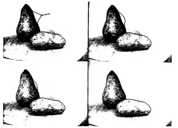
There are various tasks in image processing such as image segmentation, object tracking or object edge detection using snakes active contour model. An active contour was proposed which represents a new approach to visual analysis of shape (Kass et al., 1988).
Active contours implement image processing selectively to regions of the image, instead of processing the entire image. The basic snake model is controlled continuity spline. It is operated under external constraint forces and influence of image forces.
An initial contour in ACM solves the image plane towards the problem of object boundaries. Suitable energy terms are added so the contour corresponds to a local minimum of the functional coincides.
Figure 1.1: Edge detection using snakes active contour model (Kass et al., 1988)
the desired local minimum of the functional which coincides at the edge of the object as desired. These forces come from automatic attentional mechanisms such as a user interface or interpretation of high-level.
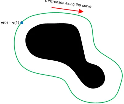
The contour is defined in the(x,y)plane parametrically asv(s) = (x(s),y(s)), wherex(s)andy(s)arex,ycoordinates of the contour andsis the normalized index of the control points. The function of energy consists of two components, internal energy and external energy. The energy functional is:
Esnake∗ =
Z 1
0
Esnake(v(s))ds =
Z 1
0
Eint(v(s)) +Eext(v(s)) =
Z 1
0
Eint(v(s)) +Eimage(v(s)) +Econ(v(s)). (1.4) .
The internal energy is defined as:
Eint= (α(s)|vs(s)|2+β(s)|vss(s)|2)/2 (1.5)
The spline energy is composed in first-order and second-order term where the first-order term is controlled by the coefficients α(s) and the second-order term is controlled by β(s). Both terms are combined to make the snake act as a membrane and a thin plate.
The weightα(s)andβ(s)should be adjusted to control the relative importance in terms of membrane and thin-plate. α(s) should be set to zero at a point to allow a snake to be a second-order discontinuous and develop a corner.
Each iteration takes implicit Euler steps to calculate the internal energy and explicit Euler steps to determine the image and external constraint energy. Three different energy functionals which attract the snake to the desired features in the image are present. The total image energy is as follows:
Eimage=wlineEline+wedgeEedge+wtermEterm. (1.6)
If set
Eline=I(x,y) (1.7)
Then, the snake will be attracted if there is either a light or dark lines depending on the sign ofwline. Based on a very simple energy functional, it can search the edges in an image. IfEedge=−| 5I(x,y)|2is set then the snake is attracted to contours with large image gradients.
(Kass et al., 1988) experimented with a slightly different edge functional to demonstrate the continuity of the relationship of scale-space to the edge detection theory. The edge energy functional is:
level lines is used to seek line segments and corners termination and can be defined by:
Eterm= ∂ θ
∂n⊥ (1.9)
where n= (cosθ,sinθ), n⊥ = (−sinθ,cosθ) and θ =tan−1(Cy
Cx) be the gradient
angle. LetC(x,y=Gσ(x,y)∗I(x,y)be a slightly smoothed version of the image.
Snake is attracted to edges or terminations created by combining Eedge and Eterm.
Figure 1.2: Parametric snake curve v(s)
A formulations of the image energy has also been proposed to improve the original model, including the Balloon force field, together with the potential forces comprising the external forces. The external forces on the original model are modified to give more stable results to push the the curve to the edges (Cohen,1991).
1.4 Fast ACM Algorithm
handle topology of the evolving contour changes because of situations where no prior knowledge of the number of objects to be detected is available.
Geometric ACM has addressed some weaknesses of the standard active contours. Geometric ACM was introduced based on the mean curvature motion equation (Caselles et al.,1993). The implicit geometric ACM, that can be associated with the explicit snake model is represented by function, is embedded into an energy functional.
(Weickert & Kuhne,2002) considered, which combined geometric and geodesic model and introduced two additional functions,aandb:
∂u
∂t =a(x)| 5u|div(
b(x)5u
| 5u| +| 5u|kg(x), (1.10)
• | 5u|div(|55uu|), is the mean curvature term of ACM which smoothes level sets, • k| 5u|describes motion in normal direction, i.e. dilation or erosion depending
on the sign ofk. Also called as balloon force for pushing a level set into concave regions or to create convex regions.
• gis a stopping function such as the PeronaMalik diffusivity.
a:=g,b:=1 are set for the results in the geometric model, ora:=1, b:=g for the results in the geodesic model. Discretizations of space and time have to be considered to provide a numerical algorithm.
1.4.1 Geometric ACM
Based on the curve evolution theory and geometric flows, the level sets are used in geometric ACM implementation to allow automatic changes in the topology(Caselles et al.,1993).
The geometric ACM equation is expressed by (Weickert & Kuhne,2002): ∂u
∂t =g(x)| 5u|div( 5u
where
g(x) = 1
1+ (5Gσ∗go)2
(1.13)
Gσ ∗go is the convolution of the image where the contour of an object O is searched with the GaussianGσ(x)andu0is the initial data.
Unlike the method of snakes that depends on many adjustment parameters, geometric ACM is stable and allows a rigorous mathematical analysis. The model allows simultaneous extraction of smooth shapes and detects several contours. As a result of the stability, it can be engineered as a method of zero parameter in the applications.
A novel algorithm using multigrid for the rapid evolution of geometric ACM implementation was proposed in order to retain accuracy and demonstrate excellent stability and rotational invariance properties even with big time steps. Internal forces are treated with implicit schemes while external forces with explicit schemes to keep the curve smooth (Papandreou & Maragos(2004).
1.4.2 Geodesic ACM
Based on energy minimization, geodesic ACM permits connections of snakes for object segmentation. The energy of the snakes model is equivalent to finding geodesic curves in a Riemannian space, which is defined by the content of image (Caselles et al.,1997).
In the implicit geodesic ACM (Weickert & Kuhne,2002) ∂u
∂t =| 5u|(div(g(x) 5u
| 5u|) +kg(x), Ω×(0,∞), (1.14)
wherekis a positive real constant.
This scheme is derived from the classical energy-based active contours and geometry curve evolution. Formulation of geodesic is to detect the edge to find a minimum weighted length of curves, improving the edges detection with large differences in their gradient. Then, this geodesic ACM is assumed to represent the zero level- set of a 3D function, and the computation of geodesic curve is reduced to a geometric flow.
To improve those models, this geodesic flow includes a new velocity curves component. The new velocity component allow accurate tracking of boundaries of the high variation in their gradient, including small gaps, a task that is difficult to achieve with the previous curve evolution models. In (Caselles et al.,1997), the level sets approach is used in order to find the geodesic curve (Osher & Sethian,1988).
The purpose ofg(x)is to stop the evolving curve when it arrives at the object boundaries. (Caselles et al.,1993) & (Malladi,R., Sethian & Vemuri,1995) chose
g(x) = 1
1+ (5Gσ∗go)2
, (1.16)
where x is a smoothed version of x and x was computed using Gaussian filtering. Gσ∗go is the convolution of the image go where we are looking for the contour of an objectOwith the GaussianGσ(x) =Cσ−1/2exp(−|x|2/4σ).
Geodesic ACM are widely used in many applications, including object segmentation and tracking in movie sequence (Goldenberg et al.,2001). The AOS scheme has been adapted to the geodesic ACM, motivated by level set approach and fast marching for re-initialization.
1.5 ACM for MRI Application
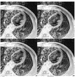
Figure 1.3: MRI application using ACM
A novel technique that combines MRI of hyper-polarized helium gas and conventional MRI facilitates high resolution imaging of lung function (Ray & Acton (2002). This application which computes the total volume of the lung cavity and the cavity volume from the proton imagery were used to calculate ventilation percentage.
Parametric snake is used in the segmentation method to measure the amount of lung air space and a classification approach to calculate the functional air space. It has a lower association with computational complexity compared to the geometric counterpart. The main weakness associated with parametric snakes is it is difficult to merge or split.
ACM is developed to find and map the outer cortex of the brain images (Davatzikos & Prince, 1995) and then to determine the spine of such ribbons. ACM has an external force derived from an integration of the data and internal elasticity forces.
(Yezzi et al., A.,1997) used a new geometric ACM, based on Riemannian metrics depending on the image and related to gradient flows for ACM. This is done by combining curve evolutionary approach to active contours and classical snake methods.
numerical methods from evolutionary level set techniques were developed by (Osher Sethian, 1982, 1984,1986, 1989), and (Malladi et al.,1995).
In (Derraz et al.,2007), coupling of geometrical ACM for image segmentation using homogenization of edge stopping map function based on the anisotropic diffusion PDE was carried out. This homogenization provides a regular velocity propagation, unique viscous solution and unique segmentation for low contrasted images. However, geometrical ACM is based on gradient information.
1.6 Direct Method and Iterative Method
Much research has focused on the development algorithms, both direct and iterative. Direct and iterative methods was used to solve a linear system of equations, in the form of Au = f with A an n by n nonsingular matrix, that form a subspace. The convergence of Krylov subspace methods depends strongly on the eigenvalue distribution ofA, and on the angles between eigenvectors ofA.
Classical direct search methods was developed during the period 1960-1971. The direct method used here is a Gaussian elimination and Thomas method applied to sparse symmetric matrices. Gaussian elimination is an algorithm for solving systems of linear equations. It can also be used to find the rank of a matrix, to calculate the determinant of a matrix, and to calculate the inverse of an invertible square matrix.
Comparison between direct and iterative methods show that the computation rate and the number of iterations are both important factors influencing the CPU time required for each solver. The computation rate was influenced by the algorithm and the data structure used for each method. While the number of iterations was influenced by the structure of the matrices and convergence rate.
The iterative methods require much less memory than direct methods and show the most promising for very large finite element models, especially if the element aspect ratios are near unity. Rapid convergence of the iterative methods makes them faster than the direct solvers (Poole,1991).
In 1975, a 3-block SOR method was proposed for solving least-squares problems based on a partitioning scheme for the observation matrix A. Preliminary works have been completed for correcting and extending the SOR convergence interval. Problem of the 3-block formulation, leading other alternative formulation to a 2-block SOR method and it is shown that the method always converges for sufficiently small SOR parameterω (Markham et al.,1985).
The successive over-relaxation (SOR) method is a variant of the Gauss-Seidel method to solve a linear system of equations and have more faster convergence than the Gauss-Seidel method. The idea is to choose a value forω that will accelerate the rate of convergence of the iterations to the solution(David & Frankel, 1950).
1.7 Multigrid Method (MG)
The boundary value problems in numerical solution are absolutely necessary in almost all development fields of physics and engineering sciences. Numerical solution is crucial to solve dimensional huge system where the system has become larger and possesses larger number of equations although the computers have become faster and vector computers are available.
Brandt, McCormick and Ruge introduced Multigrid in 1982. In 1983, it was further explored by (Stuben,1983), and then popularized by Ruge and Stuben in 1987. The basic idea of multi-level adaptive technique (MLAT) is not to work with a single grid, but with order grids of rising fineness. Brandt has shown the actual efficiency of the multigrid methods (Brandt,1997).
The basic idea is to recursively take coarser and coarser grids. Finally, combination with nested idea of iteration for a suitable algorithmization in which the computational work required to achieve the accuracy of the discretisation is proportional to the number of discrete unknowns (Trottenberg et al., 1984).
The basic idea for convergence acceleration is to get error smoothing effect of relaxation methods. This idea can be found in the early literature by Southwell (1935,1946 & 1952). Scroder has then introduced the recursive application of coarser grids for an efficient solution of specific discrete elliptic boundary value problems. But, explicit error smoothing has not yet been performed. Finally, the self-suggesting idea of nested iterations has been known for a long time.
A theory of multigrid methods to find considerations of the problem in analysis of model type is presented. For smoothing, rectangular domains and non-linear problems treatment, red black and four colour relaxation methods are used (Hackbusch, 1985).
Since 1977, multigrid methods have grown. In recent years, the field of finite elements which has first been of a more theoretical interest to multigrid methods becomes attractive for practical investigations. Apart from linear and non-linear boundary value problems, eigenvalue problems and bifurcation problems, parabolic and other time-dependent and non-elliptic problems occur in numerical fluid dynamics.
Multigrid methods also can be solved by integral equations efficiently. Furthermore, multigrid methods are suitable to solve special systems of equations without continuous background. Extension of the field of applications of multigrid methods is the combination of the multigrid idea with other numerical and more general mathematical principles such as combination with extrapolation and defect method. Finally, multigrid methods are used on vector and parallel computers for optimal use as well as to approach within the computer architecture.
as good as multigrid. The multigrid algorithm involves a new parameter (cycle index) which is the number of times the MG procedure is applied to the coarse level problem. According to Borzi(1999), the choiceN = 1 in a multigrid cycle is suitable to solve the problem to second-order accuracy.
1.8 Performance Analysis
1.8.1 Convergence Criterion
Convergence criterion is usually sought in converged solution. The concept of the convergence rates has been developed for analyzing iterative methods for solving systems of simultaneous linear algebraic equations. Its rate of convergence sequence as well as the convergence, uniqueness of the solution and error in the approximate solution are obtained after a finite number of computations(Hamilton,1984).
Many convergence rates have been proposed and some are based on the residual-norm, while others are based on the error-norm. Consider a large sparse linear system of equationsAu= f, whereAis an×nmatrix.
(1)Relative residual convergence criterion. It is defined as
Rr =
krkk2
kr0k2
= kb−Axkk2 kb−Ax0k2
≤tol, k=1,2, ...,maxit (1.17)
wheremaxitrefers to maximum number of iteration.
Based on the relationek=A−1rk , it is know that the criterion has the following error bound,
(2) Relative error-norm criterion. The relative error-norm criterion is defined based on the approximate solution as
Ri= k
xk−xk−1k∞ kxkk∞ ≤,
k=1,2, ...,maxit (1.19)
in which k.k∞. The relative error-norm criterion is closely related to the relative residual convergence criterion, but this relation also depends on the properties of matrixA.
Iterative methods for solving this problem are
u(n+1)=MU(0)+N f, (1.20)
where M and N have to be constructed in such a way that given an arbitrary initial vector u(0), the sequence u(v),v=0,1, ...,converges to the solutionu=A−1f. M is
called the iteration matrix. The following convergence criterion based on the spectral radiusρ(M)of the matrixM. The following theorem is proved by Varga (1962).
Theorem 1.8.1. If A is an(m×m), then A converges if and only if p(A)<1.
kM(k)k<ε (1.21)
Iteration process is determined by number of k iteration which satisfy the inequality below,
−logε −kA(k)k
1
k
≤k (1.22)
An optimum value of iteration, k0at convergence criterion can be approximate
by the following equation,
k0'
−logε
ρ(A) =
logε
τ(A), (1.23)
Practically, an iterative method will converge at k0 iteration, if the convergence
criterionε =10−a,α∈Z+is satisfied such that
e(k)=max|uk+1−uk|<ε, (1.25)
with u(k) and u(k+1)are previous iteration and latest iteration respectively. The best convergence rate for a comparison of iterative method is the one which gives the smallest maximum error e(k).
1.8.2 Root Mean Square Error (rmse)
The convergence rate for iterative methods is determined by computing root mean square error,(RMSE)formula. The formula is given as the following,
RMSE = s
ℵ
∑
i
(u(jk+1)−u(jk))2/ℵ, (1.26)
where ui and ui are approximation solution and exact solution respectively. For one dimensional problem ℵ=m, two dimensional ℵ=m×m, and three dimensional
ℵ=m×m×m,i=x,i= (x,y), andi= (x,y,z)respectively.
If thermse is within the error,ε, then the procedure will stop. Otherwise, the procedure will continue until this condition is reached.
1.9 Background of the problem
Firstly, it depends on its parameterization, in which the model is non-geometrically and intrinsic properties of the contour. Secondly, there is no prior knowledge of some of the detected object, so it cannot handle the topological changes in contour naturally.
In image analysis and computer vision, geometric ACM is a very popular PDE-based tool. Most of the geometric ACMs are built PDE-based on the level-set method. Computation cost can be high, which makes its utilization in time-critical applications problematic despite the advantages of the level-set method.
The Geodesic ACM’s weakness is in its stability constraints on the time step size related to explicit numerical schemes.
1.10 Research Questions
The research will explore the following questions.
1. What is active contour and how does it work?
2. How to implement the active contour using direct, iterative and multigrid method?
3. Under which condition is each active contour method satisfactory?
4. How is the performance of the active contour methods for each numerical methods?
5. Which numerical methods is the best approaches to detect edge of object ?
1.11 Objectives of the study
The objectives of this research are:
1. To implement a Semi-implicit additional operator scheme (AOS) on geodesic ACM.
computational complexity, accuracy and number of iterations.
1.12 Scope of the problem
The scope of this research revolves around detecting edges of the object using geodesic ACM based on semi-implicit additional operator scheme (AOS). This approach will be implemented with numerical methods such as direct, iterative and multigrid method to solve the tridiagonal linear system efficiently.
The methods under consideration are Gauss-elimination, Thomas, Jacobi, Gauss-Seidel and Successive-over-relaxation (SOR) and will be applied for medical image segmentation such as medical resonance image(MRI).
The experiment were run on Intel Core Duo Processor 2.0GHz and RAM 2GB. Matlab 7.6.0 (R2008a) were used as a tool to implement the algorithm. The analysis of the results are conducted in terms of numerical performance.
1.13 Originality of the research works
REFERENCES
Acton, S. T. (1998). Multigrid anisotropic diffusion. IEEE Trans. Image Process. 7(3): 280—291.
Babaud, J., Witkin, A., Baudin, M. and Duda, R. (1986). Uniqueness of the gaussian kernel for scale-space filtering.IEEE Trans. Pattern Anal. Machine Intell. PAMI-8.
Blake, A. and Isard, M. (1997).Active Contours.Springer.
Borzi, A. Introduction to Multigrid Methods, Institut furMthematik und Wissenschaftliches Rechnen, 1999. http://www.kfunigraz.ac.at/imawww/borzi/mgintro.pdf
Brandt, A. (1997). Multilevel adaptive solution to boundary value problems.Math. Of Computation. 31:333-390
Carolyn, L. P. (1999). The Level-Set Method.Journal of Mathematics155—164.
Caselles, V., Catt , F., Coll, T. and Dibois F. (1993). A geometric model for active contours. Numerische Mathematik66: 1—31.
Caselles, V., and Coll, B. (1996). Snakes in movement. SIAM J. Numer. Anal. 33: 2445—2456.
Caselles, V.,Kimmel, R. and Sapiro, G. (1997). Geodesic active contours. Int. J. Comput. Vision. 22: 61—79.
Chan, T. F. and Vese, L. A. (2001). Active contours without edges. IEEE Trans. Image Process. 10(2).
Davatzikos,C.A. and Prince,J.L. (1995). An Active Contour Model for Mapping the CortexIEEE Transactions on Medical Imaging.14(1):65-80.
Derraz, F., Taleb-Ahmed, A., Chikh, A. and Bereksi-Reguig, F. (2007). MR Images Segmentation Based on Coupled Geometrical Active Contour Model to Anisotropic Diffusion Filtering, inProceedings of Int. Conf. Bioinformatics and Biomedical Engineering. pp. 721-724.
El-Zehiry, N.(2009). MRI brain extraction using a graph cut based active contour model. Comput. Eng. & Comput. Sci. Dept., Univ. of Louisville, Louisville, KY .
Goldenberg, R.,Kimmel, R., Rivlin, E. and Rudzsky, M. (2001). Fast geodesic active contours. IEEE IP10: 1467—1475.
Hackbusch, W. (1985). Multigrid methods and applications.Berlin: Springer-Verlag.
Hoffman, J. D. (2001). Numerical Methods for Engineers and Scientists, Second Edition. Clinton: Washington.
Hackbusch, W. and Trottenberg, U. (1986). Multigrid Methods Ii, Lecture Notes in Mathematics 1228.Springer, Berlin.
Hackbusch, W.(1977). On the convergence of a multi-grid iteration applied to finite element equations. Institute for Applied Mathematics, University of Cologne, West Germany. Rep. 77-8.
Hamilton A. C. (1984). Alternative convergence criteria for iterative methods of solving nonlinear equations. Journal of the Franklin Institute, Volume 317, Issue 2, February 1984, Pages 89-103. 317(2):89-103.
Kass, M., Witkin, A. and Terzopoulos, D. (1988). Snakes: Active contour models.Int. J. Comput. Vision1: 321—331.
Kenigsberg, A. (2001). A multigrid approach for fast geodesic active contours, inCop. Mnt. Conf. on Multigrid Methods.
Leipnik, R. (1960). The extended entropy uncertainty principle.Inf. Control3, 18-25.
Malladi,R., Sethian, J. A. and Vemuri,B. C. (1995). Shape modeling with front propagation: A level set approach. IEEE Trans. Pattern Anal. Machine Intell 17: 158175.
Marr, D. and Hildreth, E. (1980). Theory of Edge Detection, in Proceedings of the Royal Society of London. Series B, Biological Sciences. 207(1167): 187—217.
Markham, T. L. , Neumann,M. , Plemmons,R. J. (1985). Linear Algebra and its Applications, Volume 69, August 1985, Pages 69:155-167.
McCormick, S.(Ed.) (1987). Multigrid Methods. Frontiers in Applied Mathematics, SIAM.Philadelphia, PA.
Milaszewicz, J. P. (1987).Linear Algebra and its Applications.93:161-170.
Mumford, D. and Shah, J. (1985). Boundary detection by minimizing functionals, in Proc. IEEE Comp. Soc. Conf. Computer Vision and Pattern Recognition (CVPR 85).IEEE Computer Society Press, Washington. 22—26.
Nilanjan, R., Acton, S. T., Altes, T. A. and De Lange, E. E. (2001). MRI ventilation analysis by merging parametric active contours, in Proceedings of International Conference on Image Processing (ICIP 2001). pp. 861—864.
Paragios, N. and Deriche, R. (1998). Geodesic Active Regions for Texture Segmentation.INRIA RR-3440.
Paragios, N. (1999). Geodesic Active Regions and Level Sets: Contributions and Applications in Artificial Vision. PhD Thesis.
Paragios, N. and Deriche, R. (2000). Geodesic active contours and level sets for the detection and tracking of moving objects. IEEE Transactions on Pattern Analysis and Machine Intelligence22(3): 266—280.
Perona, P. and Malik, J. (1987). Scale space and edge detection using anisotropic diffusion, in Proc. IEEE Comp. Soc. Workshop on Computer Vision. IEEE Computer Society Press, Washington. 16—22.
Perona, P. and Malik, J. (1990). Scale space and edge detection using anisotropic diffusion. IEEE Trans. Pattern Anal. Mach. Intell.12: 629—639.
Poole, E.L.(1991) Comparing direct and iterative equation solvers in a large structural analysis software systemComputing Systems in Engineering. 2(4): 397-408
Ray, N. and Acton, S. (2002). Active Contours for Cell Tracking, inProceedings of Fifth IEEE Southwest Symp. on Image Analysis and Interpretation.
Sethian, J. A. (1996).Level set methods.Cambridge: Cambridge University Press.
Sethian, J. A. (1996). A fast marching level set method for monotonically advancing fronts, inProc. Nat. Acad. Sci. 93: 1591—1595.
Sethian, J. A. (1999). Level set methods and fast marching methods. Cambridge: Cambridge University Press.
Stuben, K.(1983). Algebraic multigrid (AMG): Experiences and comparisons. Appl. Math. Comp. (13)419452.
Trottenberg, U., Stuben, K., Witsch, K. (1984). Software development based on multigrid method.North-Holland: Elservier Science Publishers.
Weickert, J. (1996). Anisotropic diffusion in image processing.PhD Thesis.
Weickert, J. and Kuhne, G. (2002). Fast methods for implicit active contour models In S. Osher and N. Paragios, editors, Geometric Level Set Methods in Imaging, Vision and Graphics. Springer.
Weickert, J. (2001). Application of nonlinear diffusion in image processing and computer vision.Acta Mathematica Universitatis Comenianae70(1): 33—50.
Weickert, J., ter Haar Romeny, B. M. and Viergever, M. A. (1998). Efficient and reliable schemes for nonlinear diffusion filtering. IEEE Transactions on Image Processing 7(3): 398—410.
Wesseling, P. (1992).An Introduction to Multigrid Methods. John Wiley.
Yezzi, A. Jr., Kichenassamy, S., Kumar, A., Olver, P. and Tannenbaum, A. (1997). A Geometric Snake Model for Segmentation of Medical Imagery. IEEE Trans. Medical Imaging.16( 2):199-209.