A Research
Program
for and the Process
of Building
and Testing
Grassland
Ecosystem
Models
G. M. VAN DYNE AND J. C. ANWAY
Highlight: This paper reports on the organization and operation of the U.S. International Biological Program ‘s Grassland Biome study. The study has involved in the past 8 years a large number of scientists from many disciplines
working in an integrated and data-sharing mode. Field studies have been conducted on 11 western grassland sites to obtain data to drive and to validate mathematical simulation models and to provide cross-site comparative information. The models are based upon data from field studies, the literature, and rate process studies, often conducted in the laboratory. A multiple-flow, ecosystem level model called “‘ELM” which can be adapted to various sites by changing parameters is described. The types and sources of scien tific outputs from the program are described.
Historical Aspects
The work on which we are reporting has been part of the International Biological Program (IBP) of which the United States component was organized through the National Academy of Sciences (U.S. National Committee, 1974). The part of the IBP of main interest to us here was originally called the Analysis of Ecosystems (AOE) study. There are also several other large integrated research programs in the US/IBP. The pertinent global objectives and the specific objectives of the US/IBP and the AOE study are:
@to examine the biological basis of productivity in human welfare
*to study organic matter production on a world-wide basis
eta acquire information to develop and test ecological theory
@to develop a theory of usefulness to man
*to develop a theory of energy flow, nutrient cycling, trophic structure, spatial patterns, interspecies relations, and species diversity
.to further examine the ecosystem processes by which the abo ve observed characteristics are achieved and maintained.
Authors are professor of biology and research associate, College @f Forestry and Natural Resource, Colorado State University, Fort Collins. At present, Anway is with the School of Applied Science, Canberra College of Advanced Education, Canberra, A.C.T., 2601, Australia.
This paper is based on two invited papers presented at the annual meeting of the Society for Range Management, Tucson! Arizona, February 5, 1974. This paper reports on work supported m part by National Science Foundation Grant GB-41233X to the Grassland Biome, U.S. International Biological Program, for “Analysis of Structure, Function, and Utilization of Grassland Ecosystems.”
Comments on the manuscript by Ron Sauer and BilI Hunt are appreciated.
114
Analysis of Ecosystems Studies
The original plans in this part of the US/IBP were to develop several large-scale, integrated, interdisciplinary research programs called “biome studies.” These biomes were to include grasslands, deciduous forests, coniferous forests, tundra, desert, and tropical rain forests. Programs were developed in the first of these five areas. General discussions of examples of the aims, organization, and management of these large-scale programs in the U.S. and Canada are provided by Auerbach (1971), Coupland et al., (1969), Gessel (1972), Goodall (1972), and Van Dyne (1972,1975).
Support for and Participants in the Grassland Biome Study
Our research has been supported primarily by the National Science Foundation with some inputs from the Atomic Energy Commission. We have also had cooperation from many state and federal experiment stations. The study has been an interdisciplinary, interinstitutional, integrated, basic ecosystem-oriented research program. Scientists from organizations in some 24 states have participated in the Grassland Biome field studies in 10 western states. We also have been cooperating with some 30 nations having IBP grassland projects. This paper is a general overview of progress and results, and we do not present detailed results of the work of the some 200 scientists (see Wright, 197 1, and Hendricks,
1973) who have participated in the Grassland Biome study at various times in the last 6 years.
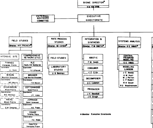
The general organizational structure during the main phases of the program divided the program into main experimental portions of (i) field validation studies, (ii) field and laboratory rate process studies, (iii) synthesis and integration efforts, and (iv) systems analysis and modelling (Fig. 1).
Grassland Biome Focus
Our original objectives included a series of broad questions which called for total-system research. No matter how narrow or detailed a single given subproject was, the relationship to the whole system was our dominant theme. A main mechanism for synthesizing our information into a whole was the use of mathematical models.
Our overall plans aimed at answering broad ecological questions. Analyses of these questions dictated early the need for detailed total system research. At the outset in 1968 it was clear that we would not be able to study all things about all
EXTERNAL AOVISORS
EXECUTIVE
CWMITTEE
FELD STUDIES
I
co “*rr[ FIELD STUMES ]
I
INTEGRATION BSYNTttEStS SYSTEMS ANUYSlS
I
SERVICES B
ADMINISTRATION
Olrector: J Ii GIBSON.
MANAGEMENT
L G Nell C B Johnson
B J Hendricks
CHEMICAL ANALYSI s W S Ferguron
D S Blgelor
STATISTICAL
DESIGN AN0
Fig. 1. Organization char; for the USIIBP Grassland Biome study during its main operational phase. The program had two major data-generation
areas (field validation studies and rate process studies) and two major areas of synthesis and analysis (integration and synthesis and systems analysis). There were s& types of centralized research supportgroups under a services and administration area.
grasslands. Our major effort was to study intraseasonal rather than interseasonal dynamics of grasslands. We put priorities, in order of decreasing importance, on biomass (carbon), energy, nitrogen, phosphorus, sulfur, and eventually other elements that move through the system. Our design has one intensive site (Pawnee) and a network of comprehensive sites (see Fig. 2).
To obtain simultaneous data sets on a comparable basis, we established a number of grassland study sites (Fig. 2). In addition, field data were obtained from other sites in rate process studies. On all sites except Dickinson, Bison, and Hays, we have collected at least 3 years of data. Several scientists have been involved in data collection on each of these sites. Table 1 places the sites into perspective by providing an overview of the grassland type, location, and coordinator.
A Systems View of Grasslands
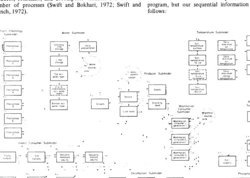
We use a systems approach as a framework for integrating our knowledge about grasslands into dynamic simulation
JOURNAL OF RANGE MANAGEMENT 29(2), March 1976
models of the ecosystem.
To characterize the systems we partitioned them into variables and constants. The variables were further divided into internal or external variables. The external or driving variables were variables “outside” the system which affect performance “inside” the system. Important external or driving variables included precipitation, solar energy input, wind, and temperature above the plant canopy, etc. Driving variables were considered “independent variables,” that is independent of the central system under study.
Next we considered a series of internal or system state variables. These are the variables inside the system which change from time to time as a response to alterations in the driving variables or the condition of other internal variables. Examples include soil water levels, herbage biomass, and animal numbers. These are the dependent variables. In a flow diagram of the system the internal or system state variables are denoted as boxes. The boxes are connected with arrows, which represent the flows of matter or energy from part to part
Fig. 2. Locations of US/IBP Grassland Biome study sites: ALE, shrub-steppe; Bison and Bridger, mountain grasslands; Cottonwood, Dickinson, and Hays, mixed prairie; Jornada, desert grassland; Osage, tallgrass prairie; Pawnee and Pantex, shortgrass prairie; and San Joaquin, annual grassland.
within the system. Each flow represents one or more rate processes within the natural system.
The items flowing in a flow diagram may be different things. They may be energy or matter; the matter may be water, carbon, nitrogen, numbers, dollars, etc.
The rate processes, i.e., the flows from one state variable to another, may be physically controlled or physiologically controlled. Examples of physical rate processes include infiltration and weathering. Examples of physiological rate processes include photosynthesis and metabolism. The rate processes causing input into a given state variable such as “live aboveground plant biomass,” for example, would include photosynthesis and translocation up from the roots. The rate processes causing outputs from this compartment would include herbivory, weathering, trampling, translocation, and
death. Each rate process can be affected by several variables. For example, photosynthesis is at various levels of resolution influenced by state variables such as leaf area, soil water, and others, and by driving variables such as solar radiation, temperature, and others.
In a mathematical description of a flow function for a given rate process, we need to use some constants or parameters. These are properties of the system that do not change during the time interval of simulation. One such constant might be the depth of the soil and the texture of the soil which we can measure in the field. Constants may also be applied to those processes whose mechanisms are unknown (e.g., nominal mortality rate) or whose level of resolution is more detailed than a system level model can reasonably encompass (e.g., a single activity factor for mammalian activity).
We also consider man to be a driving variable, or external force, in controlling certain flows to and from the system.
The system model is composed of a series of differential or difference equations which will show the change in the state variables as the functions of flows into and out of each compartment. In general, the equations in this system must each be a function directly or indirectly of the state variables, the driving variables, and time.
The Systems Process
Ecosystem simulation models are constructed largely from the results of process and literature studies and from accumulated experience. Experimental rate process studies provide data for the description of the physiological, physical, and ecological phenomena that account for transferring matter and energy within the ecosystem. These process studies may be conducted in the field or in the laboratory in a growth chamber, greenhouse, or metabolism apparatus. Such studies are designed to give the form of, and parameters values in, equations representing rate processes as the function of other variables.
Simultaneous measurements of the driving variables and state variables must be done in the field, as they cannot be obtained in the laboratory nor usually from the literature (see Table 1). The driving variable records are used as input to run or drive the models developed. The records of state variable response give us initial conditions needed to solve our difference or differential equation systems. State variable records also give results with which to compare model response.
Table 1. Sites, site characteristics, and coordinators for the US/IBP Grassland Biome study (Fig. 2).
Grassland type Site name Land ownership
Federal, ARS Federal, ARS
Coordinator
Desert grassland Shortgrass prairie
Jornada Pawnee
Mixed prairie
Pantex Cottonwood Dickinson Hays
Tallgrass prairie
Mountain grassland
Osage Bridger
Shrub-steppe
Bison’
ALE
Federal, ERDA State, South Dakota State, North Dakota State, Kansas
Private
Federal, FS
Federal, BSFW Federal, ERDA
R. D. Pieper D. A. Jameson J. L. Dodd E. W. Huddleston J. K. Lewis W. C. Whitman G. W. Tomanek G. K. Hulett P. G. Risser
D. D. Collins T. W. Weaver M. S. Morris T. P. O’Farrell
Site description reference
Herbe and Pieper 1970 Jameson 1969
Huddleston 1970 Lewis 1970 Whitman 1970 Tomanek 1970
Risser 1970
Collins 1970
Morris 1970
Rickard and O’Farrelll970
Annual grassland San Joaquin Federal, FS
‘Transitional between northwest bunchgrass and mountain grassland.
W. H. Rickard
D. A. Duncan Duncan 1975
Models utilizing the data in this way predict the dynamics of the system’s state variables. Models can be validated by comparing model output with the measurements made in the field. This comparison leads, in subsequent years, to both model modification and redesign of field and laboratory studies. We will give later some examples of output from our simulation models. We also note here that we use optimization models in our studies, but their description is beyond the scope of this paper (see, for example, Swartzman and Van Dyne, 1972, 1975).
Treatments and Testing Hypotheses
Conducting an intensive survey of an ecosystem even in great detail gains only a limited amount of information about interrelations of structure, function, and utilization. Hypotheses about interrelations of structure, function, and utilization can be developed from intensive surveys, and inclusion of experimental stress treatments allows testing of such hypotheses. In each major field study we included a minimum set of treatments or stresses on the system, and within each treatment we measured a selected set of abiotic, producer, consumer, and decomposer variables and a certain number of processes (Swift and Bokhari, 1972; Swift and French, 1972).
Plant Phenology Submodel L,
Water Submodel
We selected for inclusion in our design what we considered would be the most important stresses in grasslands which we could accomplish within our expected financial and time framework. At each major field study site, we investigated replicated areas where there had been very limited or no grazing by large herbivores for many years (excellent or good condition ranges) vs intensive or heavy grazing by large herbivores (fair or poor condition ranges). Other stress treatments were included on certain sites, especially Pawnee. These included nitrogen fertilization, irrigation, herbicides, insecticides, and other levels of grazing intensity. Our models were developed to predict general responses to these kinds of stresses.
We have two replicates of each of the two treatments on any given site. Thus, data from that site may be analyzed independent of data from other sites. We also make comparisons of all treatments of all sites and all types. Having sites in each of seven types of grasslands provides us the opportunity to make statistically designed comparison of phenomena. We are further interested in fully interrelating or correlating these data with information in the literature.
Some Outputs from the Program
We cannot detail here many of the outputs from the program, but our sequential information flows generally as follows :
Temperature Submodel AbIotic Drlwng Variables
_
Decomposer Submodel Phosphorus Submodel
(i) A periodic Newsletter listing talks, publications, and reports, and describing major programmatic activities.
(ii) More than 300 technical reports to date, which include the data and brief descriptions from individual subprojects. These reports may be obtained on loan from the library at Colorado State University; the call number is SB197/15 Tech. Rep. No. catalogued in the author and serial record as Internationa; Biological Programme, Grassland Biome, Technical Reports.
(iii) More than 100 theses and dissertations in the many institutions involved in this study to date.
(iv) More than 160 preprints of selected papers submitted for journal publication, for internal distribution only.
(v) More than 300 publications to date.
(vi) About 10 monographic type papers, across sites or across trophic levels, synthesizing results planned or in development.
(vii) We have also produced three summary volumes to date (Dix and Beidleman, 1969, 1970; Coupland and Van Dyne, 1970; French, 1971), and now we are preparing synthesis volumes on each of the seven grasslands types we have studied. In each of these volumes, we include the condensed data and information we have learned about the driving variables, state variables, rate processes, and models for that particular type of grassland. We also integrate and interrelate this information to that available in the literature. We also plan a synthesis volume on our overall cross-type, total-system comparisons.
(viii) We also produce periodically major progress reports, which include a list of technical reports, preprints, theses and dissertations, talks, and publications from the program. Progress reports and continuation proposals are available on loan from the library at Colorado State University; the call numbers are SB197/V35, SB197/V352, and SB197/V353, catalogued in the author records as George M. Van Dyne and in the title record as “Analysis of Structure, Function, and Utilization of Grassland Ecosystems.” A partial listing of publications, investigators, and summary of results is available in U.S. National Committee (1974).
Ecosystem Level Model: ELM
We have developed more than 50 models of grassland systems and major subsystems. But our substantial effort has been toward a multiple-flow, ecosystem-level model which can be adapted to various sites primarily by changing parameter values. An overall diagram of our main ecosystem level model shows some of the complexity of the system (Fig. 3). The model, for all its complexity, is still very much simplified. The model was built to address the effect on net or gross primary production of influences such as type and level of herbivory, soil water, temperature, and added nitrogen and phosphorus. ELM is considered a total system model as the abiotic, producer, consumer, decomposer, and nutrient components are all represented: (i) The abiotic submodel simulates the abiotic variables by a water flow submodel and a heat flow submodel which are stratified through the air, vegetation canopy, and soil profile (upper center, Fig. 3). (ii) The producer submodel considers carbon and phenological dynamics of both aboveground and belowground parts of a variable number of primary producers (center and upper left, Fig. 3). (iii) The decomposer submodel calculates the decomposition rates and microbe biomass in litter and dead material both above and below ground (lower center, Fig. 3). (iv) In the mammalian consumer submodel and the
118
grasshopper submodel we simulate organismal,
intrapopulation, and interpopulation dynamics of consumers (center and lower left, (Fig. 3). (v-vi) The nitrogen and phosphorus submodels simulate nutrient flow through the system (lower right, Fig. 3).
Each submodel interacts with the other six submodels to give the total model. An early version of the model has been described in detail (Anway et al., 1972) and simplified descriptions are given by Innis (1972, 1975). A preliminary mammal submodel was reported by Anway (1973) and the producer submodel by Sauer (1973). The model is being adapted for various types of grasslands, but the example graphs of model output that follow all are for shortgrass prairie on the Pawnee Site. This version of the model is described in detail in papers submitted for publication.’
Abiotic Submodel
A part of the abiotic submodel which simulates flow of water through the vegetation canopy and the soil layers is structured to include the important feedback mechanism between the biotic and abiotic state variables. The allocation of rainfall and the evaporation of water are the important processes considered. Daily rainfall, relative humidity, cloud cover, wind speed, and maximum and minimum air temperatures are used as driving variables.
Producer Submodel
Carbon and phenological dynamics of the primary producers are simulated for up to 10 species or groups concurrently. The producers can be changed as a model is adapted to different grassland sites. The dynamics of the following state variables are simulated for each species or group: live shoots, standing dead shoots, live roots, seeds, and crowns. In addition, litter and dead root variables are simulated for all producer species combined. The processes simulated are gross photosynthesis, shoot respiration, shoot to crown translocation, shoot to root translocation, shoot death, crown death, root respiration, root death, seed growth, seed germination, and the fall of standing dead to litter.
The phenology submodel simulates qualitative information and is used to regulate seasonal activity of the producer species. Seven phenological stages are considered, from winter dormancy and early vegetative growth through flowering and fruiting and then through senescence. The progression of
1 Manuscripts submitted to Ecological Monographs for consideration for joint uublication :
0 l l l l l l l l l l l
Anway, J. C. A canonical mammalian model. 82 ms. p.
Cole, C. V., G. S. Innis, and J. W. B. Stewart. Simulation of phosphorus cycling in semiarid grasslands. 61 ms. p.
Hunt, H. W. A simulation model for decomposition in grasslands. 62 ms. p.
Innis, G. S. Behavior and response of ELM: A simulation model for grasslands. 51 ms. p.
Innis, G. S. Rationale and procedures for building a simulation model for grasslands. 18 ms. p.
Innis, G. S., and J. D. Gustafson. Compartmental-flow/event- oriented simulation language: SIMCOMP 3.0. 24 ms. p.
Parton, W. J. Abiotic section of the ELM grassland system model. 51 ms. p.
Reuss, J. O., and G. S. Innis. A grassland nitrogen flow simulation model. 41 ms. p.
Rodell, C. F. A grasshopper model for a grassland ecosystem. 73 ms. p.
Sauer, R. H. A simulation model for grassland primary producer phenology and biomass dynamics. 97 ms. p.
Steinhorst, R. K., H. W. Hunt, and G. S. Innis. Sensitivity analyses of the ELM model. 44 ms. p.
Woodmansee, R. G. Critique and analysis of the grassland ecosystem model ELM 73. 52 ms. p.
40r 32 -
6-
1
40 360I
= meon and 95% confidence interval - = model prediction
1970 1971
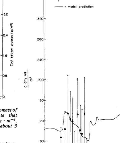
FQ. 4. Comparison of 2-year dynamics of live aboveground biomass of carbon in warm-season and cool-season grasses Note that warm-season grasses reach peak standing crops of about 30 g l m+,
whereas cool-season grasses reach peak standing crops of about 3 g l m+.
phenophases is regulated by maximum air temperature, insolation, soil water potential, and soil temperature. The biomass of the model species may be distributed or proportioned through several phenophases simultaneously.
An example of the dynamics of warm-season grass and cool-season grass live aboveground vegetation is shown (Fig. 4). Differences in climatic conditions between years cause the differences in the standing crop dynamics. The cool-season grasses grow earlier in the year and reach their peak standing crop (live + dead) at an earlier date than do the warm-season grasses. The cool-season grasses show relatively more response to favorable growing conditions in the fall of each year.
An example of the dynamics of the litter compartments is shown (Fig. 5) and compared to the 95% confidence limits based on field sampling for the same treatment. Note that biomass of litter greatly exceeds combined biomass of standing live herbage of grasses (compare Figs. 4 and 5) and that there is a high plot-to-plot variability in the litter as denoted by the large confidence intervals on field measurements.
Consumer Submodels
The mammalian submodel considers relationships and functions which are common to all mammalian consumer types. Submodels for mammals, insects, nematodes, and birds have been developed, but as of this writing only mammals and insects are incorporated in ELM. The assumption is mammal consumers affect grasslands primarily through food intake and animal products. The principal control on these processes is metabolism or energy balance, which is influenced in turn by air temperature, animal weight, wastes, activity, reproductive state, population density, animal phenology, hunger, potential intake amount, food availability or accessibility, preference, and digestibility of foods.
Figure 6 shows an example of a prediction of a consumer variable. Cattle weight (not weight gain) expressed in kilograms of carbon per head is shown for a heavy grazing treatment on a shortgrass prairie in 1970.
The objectives of the grasshopper submodel are to consider what effect grasshoppers have on the functioning of the total system and to use the model as a means for estimating the
I60
T
Fig. 5. Aboveground litter dynamics for a 2-year simulation with mean field values and confidence intervals at each sampling date.
energy flow via grasshoppers through the ecosystem. Daily air temperature and moisture conditions are important factors and have a direct influence on the flows involving forage intake, litter production, and life cycle phenomena (hatching, development, sexual maturation, egg laying, and mortality). The close agreement of model prediction and field data for grasshopper biomass dynamics over time is shown in Figure 7. Food selection in the various consumer submodels is a function of several factors. The food categories utilized are determined by the characteristics of the consumer being modelled. The quantity chosen from any of 1 to 15 food
I I I I I J
APr May Jun Jul WI SeP
Table 2. Bimonthly averages of percentage intake by food category for the grasshopper mouse, Onychomys. D column = May 1969 to April 1970 data (Flake 1973). M column = model results (in italics).
Jan.-Feb. March-April May-June July-Aug. Sept.-Oct. Nov.-Dec.
Food categories D M D M D M D M D M D M
Warm-season grasses 4 3 2 ; 3 6 7 12 7 4 4 13
Cool-season grasses 6 2 7 1 6 1 1 1 2 4 6
Forbs 9 3 3 1 6 6 7 8 7 6 8 13
Seeds 25 24 15 15 3 0 4 7 12 12 16 45
Spiders 3 3 3 1 3
Leafhoppers 6 3 6
4” :
2 0 :
3 1 4 1
1 1 1 1
Lepidoptera larvae 4
2: if:
16 18
z
1 4;
2 6 1
Coleoptera 30
t?;
54 56 40 39 3: 5
Grasshoppers 12 29 23 12 20 21 20 27 29 23 15
categories is influenced by amount of food available, food
maturity, consumers’ physiological status, and climatic conditions.
depth. Belowground, the decomposers feed on roots and other organic material depicted in the model as belowground litter.
Table 2 gives an example of prediction of food intake composition. Data are given there for model and field sampling. There is reasonable agreement between predicted
percentage composition and actual composition of the diet in
most instances.
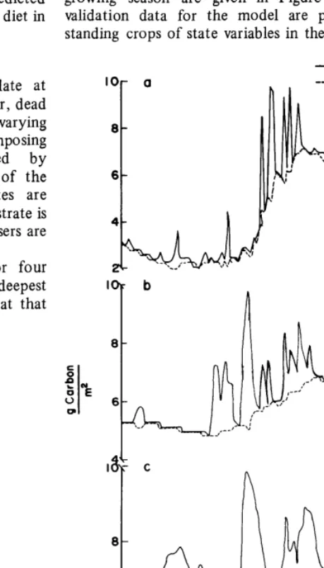
It is not easy to measure microbial biomass directly in the field, but a main byproduct of microbial activity, CO*, can be measured. Observed and predicted COZ evolution for the 1972 growing season are given in Figure 9. In most instances validation data for the model are provided by measuring standing crops of state variables in the field (e.g., see Fig. 5),
Decomposer Submodel - Total dectxtwoS8~
The decomposer submodel is designed to simulate at various soil depths the dynamics of belowground litter, dead roots, and decomposer biomass, which have varying proportions of a rapidly and a slowly decomposing component. Decomposition rates are influenced by temperature, water tension, and the concentration of the inorganic nitrogen. The decomposer biomass states are
“active” and “inactive.” During periods of activity, substrate is
assimilated and the respiration rate is high. Decomposers are
susceptible to death by freezing, drying, and starvation.
IOr a --- Inactive deC0nVOSO~
Decomposer biomass is plotted in Figure 8 for four different depths. Note the lower biomass values at the deepest layer and the lesser seasonal fluctuations in biomass at that
Fig. 7. Grasshopper biomass dynamics with model prediction (curve) and field data (points).
JOURNAL OF RANGE MANAGEMENT 29(2), March 1976
6.44
,972
Fig. 9. Model predictions and field measurements of CO, flux from the soil, measured in grams CO, per square meter per day, for the 1972 growing season. Precipitation values are also plotted at the bottom of the graph.
but it is also possible to measure for validation purposes a flux rate (e.g., see Fig. 9).
Nitrogen and Phosphorus Submodels
The nitrogen submodel incorporates eight major kinds of state variables of which five major belowground compartments are further divided into four subcompartments representing four depth layers. The depths represented by these subcompartments may be varied according to the characteristics of the site being considered. All nitrogen flows are described as a function of one or more of the following: time, soil temperature, soil water, daily growth, death or decomposition, and nitrogen or phosphorus content. Nitrogen concentrations for each biotic compartment are internally calculated, and can be used as control parameters by the respective biotic submodel. Example nitrogen model output is shown in Figure 10. Seasonal variability for amounts of nitrogen in shoots is greater than that in roots. Nitrogen in
- Live root N - - Live shoot N --- Soil NH, ... Soil ND,
1970 1971 1972
Fig. 10. Example dynamics of four nitrogen compartments over a j-year simulation run.
plants is more variable over time than in soil.
The phosphorus submodel incorporates 12 major state variables. The seven major belowground compartments are divided into three depth layers. The variables in the phosphorus submodel have dynamics similar to the equivalent variables in the nitrogen submodel.
Current Stat us-Grassland Ecosystem Models
The complexity and size of the ELM model may be illustrated in a number of ways. The flow diagram (Fig. 3) is a simplified picture of the approximately 180 state variables, 400 flows, and 500 parameters actually incorporated in the model. Simulations may be run from l-day to 5-year time-spans, with a two-year simulation with a 2day time step requiring approximately 7 minutes of machine time (compiling and running but not input-output time) on a CDC 6400. At the present time the model has about 20 man years of effort in its implementation and reporting. This does not include development of earlier models which provided a starting point. The utility of ELM will be affected by completion of work in progress and in the future. Work in progress includes adaptations to several grassland sites; results of runs of these adaptations will be incorporated in the synthesis volumes of these grassland types. Contributions to the scientific literature will require considerable time for full evaluation. Considerable guidance to research has already been provided by these modelling efforts within the Grassland Biome study. The modelling process detected many areas of research needed for improving our comprehension of North American grasslands.
Retrospect and Prospect
Our experiments, based on hypotheses derived from ecological theory and resource management experience, result in data which are analyzed by either experimental design models or least squares prediction models. We have used various statistical models to derive parameters and equations to be used subsequently to structure either simulation models or optimization models. These equations may be either individual equations which are part of a total model, or they may be part of a single equation in the total model. Eventually we will need to combine simulation and optimization models into resource system management models. There is feedback to ecological theory and to resource management from the development and running of both systems simulation and optimization models. Large, interdisciplinary research programs, such as the Grassland Biome study, should result in the development of new, improved, or more quantitative ecological theory, and eventually better resource management. Early programmatic synthetic output already is being used in development of environmental impact statements. Overall, this long-term study has had three phases: “feasibility, respectability, and utility.” We are convinced we have demonstrated the feasibility of doing this kind of research and producing a large amount of data. We are now in the process of demonstrating the respectability of the data and the models. We have yet to make full utilization of our results. The IBP terminated July 1974 as a formal program, but we hope to have through 1976 to finalize field and laboratory studies and to publish and reflect upon our results.
too much of it. There is now a major job in condensing it and making it available to the scientific and resource management
Innis, G. S. 1972. ELM: A grassland ecosystem model. Presented at 1972 Summer Computer Simulation Conf., 14-16 June, San Diego,
community. It will take time and a group of ibiased individuals at the national or international levels knowledgeable about these programs to make the final judgments and interpretation of our results.
Literature Cited
Calif.
Innis, G. S. 1975. Role of total systems models in the Grassland Biome
study, p. 13-47. In: B. C. Patten (Ed.) Systems analysis in simulation in ecology. VoL 3. Academic Press, Inc., New York.
Jameson, D. A. (Coordinator). 1969. General description of the Pawnee Site. US/IBP Grassland Biome Tech. Rep. No. 1. Colorado State Univ., Fort Collins. 32 p.
Anway, J. C 1973. Consumer simulation model: A canonical model, p.
835-840. In: Proceedings of the 1973 Summer Computer
Simulation Conference. Vol. II. Simulation Councils, Inc., La Jolla, Calif.
Anway, J. C., E. G. Brittain, H. W. Hunt, G. S. Innis, W. J. Parton, C. F. Rodell, and R. H. Sauer. 1972. ELM: Version 1.0. US/IBP Grassland Biome Tech. Rep. No. 156. Colorado State Univ., Fort Collins. 285 p.
Lewis, J. K. 1970. Comprehensive network site description,
Cottonwood. US/IBP Grassland Biome Tech. Rep. No. 39. Colorado
State Univ., Fort Collins. 26 p.
Morris, hi. S. 1970. Comprehensive network site description, Bison.
US/IBP Grassland Biome Tech. Rep. No. 37. Colorado State Univ., Fort Collins. 23 p.
Rickard, W. H., and T. P. O’Farrell. 1970. Comprehensive network site
description. ALE. US/IBP Grassland Biome Tech. Rep. No. 36.
Auerbach, S. I. 1971. The deciduous forest biome program in the Colorado State Univ., Fort Collins. 5 p.
United States of America. p. 677-684. In: Productivity of the forest Risser, P. G. 1970. Comprehensive network site description, Osage.
ecosystems of the world. Proceedings Brussels Symposium, 1969. US/IBP Grassland Biome Tech. Rep. No. 44. Colorado State Univ.,
UNESCO Ser. Ecol. Conserv., No. 4. Paris, France. Fort Collins. 5 p.
Collins, D. D. 1970. Comprehensive network site description, Bridger.
US/IBP Grassland Biome Tech. Rep. No. 38. Colorado State Univ., Sauer, R H. 1973. PHEN: A phenological simulation model. p.
Fort Collins. 10 p. 830-834. In: Proceedings of the 1973 Summer Computer
Coupland, R. T., R. Y. Zacharuk, and E. A. Paul. 1969. Procedures for Simulation Conference. Vol. II. Simulation Councils, Inc., La Jolla,
study of grassland ecosystems. p. 25-47. In: G. M. Van Dyne (Ed.). Calif.
The ecosystem concept in natural resource management. Academic S war tz man, G. L., and G. M. Van Dyne. 1972. An ecologically based
Press, Inc., New York. simulation-optimization approach to natural resource planning.
Coupland, R. T., and G. M. Van Dyne (Ed.). 1970. Grassland S wa Annu. Rev. Ecol. Syst. 3:347-398. rt
ecosystems: Review of research. (Proc. September 1969 Meeting PT zman, G. L, and G. M. Van Dyne. 1975. Land allocation
Grasslands Working Group, In ternat ional Biological Programme, decisions: A mathematical programming framework focusing on
Saskatoon and Matador, Saskatchewan, Canada.) Range Sci. Dep. quality of life. J. Environ. Manage. 3: 105-l 32.
Sci. Ser. No. 7. Colorado State Univ., Fort Collins. 208 p. Swift, D. M., and U. G. Bokhari. 1972. Basic sample collection and
Dix, R L., and R. G. Beidleman (Ed.). 1969. The grassland ecosystem: handling procedures for the Grassland Biome 1972 season. US/IBP A preliminary synthesis. Range Sci. Dep. Sci. Ser. No. 2. Colorado
Grassland Biome Tech. Rep. No. 146. Colorado State Univ., Fort
State Univ., Fort Collins. 437 p. Collins. 17 p.
Dix, R. L., and R. G. Beidleman (Ed.). 1970. The grassland ecosystem: Swift, D. M., and N. R French (Coordinators). 1972. Basic field data
A preliminary synthesis. A. supplement. Range Sci. Dep. Sci. Ser.
collection procedures for the Grassland Biome 1972 season. US/IBP
No. 2 Supplement. Colorado State Univ., Fort Collins. 110 p. Grassland Biome Tech. Rep. No. 145. Colorado State Univ., Fort Collins. 86 p.
Duncan, D. A. 1975. Comprehensive network site description, San Tomanek, G. W. 1970. Comprehensive network site description, Hays.
Joaquin. US/IBP Grassland Biome Tech. Rep. No. 296. Colorado US/IBP Grassland Biome Tech. Rep. No. 41. Colorado State Univ.,
State Univ., Fort Collins. 15 3 p.
Flake, L. D. 1973. Reproduction of four rodent species in a shortgrass prairie of Colorado. J. Mammal. 55(1):213-216.
French, N. R. (Ed.). 1971. Preliminary analysis of structure and function in grasslands. Range Sci. Dep. Sci. Ser. No. 10. Colorado State Univ., Fort Collins. 387 p.
Gessel, S. P. 1972. Organization and research program of the western
Coniferous Forest Biome, p, 7-14. In: G. F. Franklin, L. F.
Dempster, and R. H. Waring (Ed.). Research on Coniferous Forest ecosystems: First year’s progress in the Coniferous Forest Biome, US/IBP. Pacific Northwest Forest and Range Exp. Sta., Forest Serv., U.S. Dep. Agr., Portland, Ore.
Goodall, D. W. 1972. Building and testing ecosystem models, p.
173-194. In: J. N. R. Jeffers (Ed.). Mathematical models in ecology.
Blackwell Sci. Publ., Oxford, England.
Hendricks, B. J. (Compiler). 1973. Curriculum vitae of scientists who participated in the U.S. IBP Grassland Biome studies for 1971 and
1972. US/IBP Grassland Biome Tech. Rep. No. 223. Colorado State
Univ., Fort Collins. 302 p.
Herbel, C. H., and R D. Pieper. 1970. Comprehensive network site description, Jornada. US/IBP Grassland Biome Tech. Rep. No. 43. Colorado State Univ., Fort Collins. 21 p.
Huddleston, E. W. 1970. Comprehensive network site description,
Pantex. US/IBP Grassland Biome Tech. Rep. No. 45. Colorado State Univ., Fort Collins. 12 p.
Fort Collins. 6 p.
U.S. National Committee. 1974. U.S. participation in the International Biological Program. National Academy of Sciences U.S. Nat. Comm. I.B.P. Rep. 6. 166 p.
Van Dyne, G. M. 1972. Organization and management of an integrated
ecological research program-with special emphasis on systems
analysis, universities, and scientific cooperation, p. 111-172. In: J.
N. R. Jeffers (Ed.). Mathematical models in ecology. Blackwell Sci. Publ., Oxford, England.
Van Dyne, G. M. 1975. Some procedures, problems, and potentials of
systems-oriented, ecosystem-level research programs. p. 4-58. In:
Procedures and examples of integrated ecosystem research.
Barrskogslandskapets Ecologi Tech. Rep. 1 (Swedish Coniferous
Forest Project), Uppsala, Sweden.
Whitman, W. C 1970. Comprehensive network site description,
Dickinson. US/IBP Grassland Biome Tech. Rep. No. 40. Colorado State Univ., Fort Collins. 15 p.
Wright, R G. (Compiler). 1971. Curriculum vitae of scientists to
participate in the U.S. IBP Grassland Biome studies proposed for 1972 and 1973. US/IBP Grassland Biome Tech. Rep. No. 125. Colorado State Univ., Fort Collins. 266 p.