Study of Neural Network Size Requirements for Approximating Functions Relevant to HEP

Study of Neural Network Size Requirements for

Approxi-mating Functions Relevant to HEP

JessicaStietzel1,2,∗_{and KevinLannon}2,∗∗

1_{College of the Holy Cross} 2_{University of Notre Dame}

Abstract. Neural networks, and recently, specifically deep neural networks,

are attractive candidates for machine learning problems in high energy physics because they can act as universal approximators. With a properly defined ob-jective function and sufficient training data, neural networks are capable of

ap-proximating functions for which physicists lack sufficient insight to derive an

analytic, closed-form solution. There are, however, a number of challenges that can prevent a neural network from achieving a sufficient approximation of

the desired function. One of the chief challenges is that there is currently no fundamental understanding of the size—both in terms of number of layers and number of nodes per layer—necessary to approximate any given function. Net-works that are too small are doomed to fail, and netNet-works that are too large often encounter problems converging to an acceptable solution or develop is-sues with overtraining. In an attempt to gain some intuition, we performed a study of neural network approximations of functions known to be relevant to high energy physics, such as calculating the invariant mass from momentum four-vector components, or calculating the momentum four-vector vector of a parent particle from the four-vectors of its decay products. We report on the results of those studies and discuss possible future directions.

1 Introduction

An artificial neural network (ANN) can be viewed as a universal function approximator. In other words, an ANN is a function with many free parameters that can be tuned so that, assuming a large enough ANN, it can learn to approximate any reasonable function. Fig. 1 depicts a basic ANN, which can also be expressed using the following set of equations:

yj=h    2

i=0

Aj,ixi+aj  

 (1)

zk=

2

j=0

Bk,jyj+bk (2)

h(x)=

 

0x xx≤>00 (3)

The Ai,j andBk,l represent free parameters that can be tuned (referred to as weights) that multiply the appropriate input values to the layers. Theaiandbjare additional free param-eters referred to as biases that can shift the weighted sum of inputs. The functionh(x) is a non-linear function typically called an activation function. All ANNs in this study use the rectified linear (ReLU) activation function. The weights and bias parameters are learned by applying the ANN to example inputs and adjusting these parameters to minimize the diff

er-ence between the network output and the desired output. An ANN with more than one hidden layer is often referred to as a deep neural network (DNN).

Deep Learning



Neural networks as function

approximator



Learns from map of inputs and

outputs



Outputs given by

1

x

x

x

y

y

y

y

y

y

z

z

z

A

A

B

B

a

b

2

Input Hidden Output

Bias

Figure 1.A diagram depicting a simple ANN.

There is a growing interest in DNN techniques in high energy physics (HEP). There is a long history in HEP of using multivariate analysis (MVA) techniques, including ANNs as well as other techniques like boosted decision trees (BDTs) to address classification prob-lems, e.g. separating collisions resulting from a process of interest (signal) for other similar collisions (background). A specific study that was the inspiration for this study is given in [1]. An intriguing conclusion of this study was that a DNN trained only with basic inputs (e.g. particle four-vectors) can perform at least as well as other techniques (shallow ANN or BDT) trained using variables specifically engineered to perform well in MVA separation. The implication is that intermediate hidden layers in the DNN are effectively constructing their

own “engineered” variables to aid in the separation. This is a particularly attractive idea in HEP because obtaining useful engineered variables can be a time-consuming manual exercise which perhaps a DNN can learn automatically.

To realize the potential implied by the studies in [1], however, does require some work. Instead of spending time searching for useful engineered variables, someone using a DNN with basic components must instead explore the space of DNN parameters (number of nodes in each layer, number of layers, and topology of the connections between nodes). Roughly speaking, if a DNN is too small (too few layers or too few nodes in each layer) then it may not have enough flexibility to approximate the desired function. On the other hand, if the network size chosen is significantly larger than needed, computational issues training large DNNs may prevent the learning procedure from arriving at an optimal set weights to produce the desired function. Beyond considerations of network size and topology, there are

The Ai,j andBk,l represent free parameters that can be tuned (referred to as weights) that multiply the appropriate input values to the layers. Theaiandbjare additional free param-eters referred to as biases that can shift the weighted sum of inputs. The functionh(x) is a non-linear function typically called an activation function. All ANNs in this study use the rectified linear (ReLU) activation function. The weights and bias parameters are learned by applying the ANN to example inputs and adjusting these parameters to minimize the diff

er-ence between the network output and the desired output. An ANN with more than one hidden layer is often referred to as a deep neural network (DNN).

Deep Learning



Neural networks as function

approximator



Learns from map of inputs and

outputs



Outputs given by

1

x

x

x

y

y

y

y

y

y

z

z

z

A

A

B

B

a

b

2

Input Hidden Output

Bias

Figure 1.A diagram depicting a simple ANN.

There is a growing interest in DNN techniques in high energy physics (HEP). There is a long history in HEP of using multivariate analysis (MVA) techniques, including ANNs as well as other techniques like boosted decision trees (BDTs) to address classification prob-lems, e.g. separating collisions resulting from a process of interest (signal) for other similar collisions (background). A specific study that was the inspiration for this study is given in [1]. An intriguing conclusion of this study was that a DNN trained only with basic inputs (e.g. particle four-vectors) can perform at least as well as other techniques (shallow ANN or BDT) trained using variables specifically engineered to perform well in MVA separation. The implication is that intermediate hidden layers in the DNN are effectively constructing their

own “engineered” variables to aid in the separation. This is a particularly attractive idea in HEP because obtaining useful engineered variables can be a time-consuming manual exercise which perhaps a DNN can learn automatically.

To realize the potential implied by the studies in [1], however, does require some work. Instead of spending time searching for useful engineered variables, someone using a DNN with basic components must instead explore the space of DNN parameters (number of nodes in each layer, number of layers, and topology of the connections between nodes). Roughly speaking, if a DNN is too small (too few layers or too few nodes in each layer) then it may not have enough flexibility to approximate the desired function. On the other hand, if the network size chosen is significantly larger than needed, computational issues training large DNNs may prevent the learning procedure from arriving at an optimal set weights to produce the desired function. Beyond considerations of network size and topology, there are

also questions of other network hyperparameters, like the choice of activation function or regularization techniques. There is, as they say, no free lunch.

Unfortunately, there is no first principles technique for estimating the size of network needed to approximate any given known function. Furthermore, the functions the network needs to approximate are not known in advance. (After all, if we knew these functions, we wouldn’t need a DNN.) Therefore, the standard approach taken to determine the best network size and topology is trial and error. Lacking a more methodical approach to the problem, it might be beneficial to undertake studies at least to build some guiding intuition. The goal of this paper is to examine how ANNs can approximate some simple functions commonly encountered in HEP to develop some guiding intuition.

2 Studies

The studies performed are detailed below. In each study, the input consisted of a triplet of three numbers which could be thought of as representing the information contained in a three-dimensional momentum vector. The values of the three numbers are chosen to represent ranges typical for momentum vectors of particles from an LHC experiment. However, during the training process, all input values are standardized. That is, a linear transformation is applied to each component of the input vector such that the distribution of that component has a mean of zero and and standard deviation of one.

Vector to Vector:The ANN is trained to reproduce the input vector:yi=xi

Vector to Vector2_{:The ANN is trained to calculate a vector containing the square of the} input vector. In other words,yi=x2_i.

Vector to|Vector|2_{:The ANN is trained to calculate the magnitude of the vector from its} components. The output of the ANN in this case is a single number:

y=

3

i=1 x2

i

Although these functions are very simple, they represent some of the most basic operations that might be performed on particle physics data consisting of momentum vectors for parti-cles.

In each of the studies, the ANN training proceeds as follows: The networks are defined with the Keras [2] software and the training is accomplished via the Theano [3] backend. The mean-squared-error (MSE) loss function is used in the training, and the ANNs are optimized with mini-batch gradient descent using the ADAM [4] algorithm with the default parameters. The training sample always consists of one million examples and a validation sample of 10,000 examples is used to track the network performance during training. For each study, five trials with different randomly generated initial weights are run, and when a single network

must be chosen, the one with the best validation loss is considered. For each study, a mini-batch size of 1,000 is used and the ANN is trained for 5,000 epochs. The weights from the epoch with the smallest validation loss are used for the final trained ANN.

2.1 Vector to Vector:

network topology from Fig. 1. The obvious solution is just to haveAandBweight matrices diagonal, with the bias parametersachosen to shift the inputs so that they are always positive and the bias parametersbchosen to undo the shift froma. In other words:

A=

  

1 0 0 0 1 0 0 0 1  

 a=

  −

x0,min

−x1,min

−x2,min  

 B=

  

1 0 0 0 1 0 0 0 1  

 b=

  

+x₀,min

+x₁,min

+x₂,min  

 (4)

Surprisingly, examining the outcome of any of the five trials of training an ANN to solve the problem reveals a very different set of weights and bias parameters. For example, one

randomly selected trial obtained the following weights.

A=

  

0.711 0.279 0.266 0.023 0.494 −0.102

−0.091 0.354 0.471  

 a=

  

1.474 1.929 1.448  

 (5)

B=

  

1.313 −0.182 −0.782

−0.009 1.754 0.386 0.260 −1.354 1.682  

 b=

  −

2.294

−1.154

−2.203  

 (6)

This is a surprising result, at least at first consideration, but it can easily be verified that an ANN using these weights and bias parameters does in fact accomplish the objective of mapping the inputs to the outputs. Some clarity can be obtained by considering that although Eq. 4 certainly solves the problem, it is not the only solution. A small amount of algebra reveals any solution for which the weights and bias parameters satisfy the following equations will be a valid solution:

AB=I Ba+b=0 (7)

Many possible ANN trainings satisfy Eq. 7 without being identical to the solution from Eq. 4. A lesson that can be extracted from this study is that when an ANN approximates a function, there is no guarantee that it will use the same strategy that a human would choose in extracting the solution. Furthermore, if there is some knowledge about the symmetries in the data or relationships among the inputs (e.g. the inputs are completely independent so that each output should only be connected to one input), that knowledge can be leveraged to substantially simplify the problem at hand. For example, in this case, using our knowledge that the inputs are completely independent and that we’re just trying to reproduce them with this ANN, we could have deduced the structure in Eq. 4 and the only parameters that would need to be discovered through training are the bias parameters.

2.2 Vector to Vector2

This study involves solving a problem that is not so straightforward to solve by inspection. However, because of the ReLU activation functions used in these ANNs, and restricting the study only to ANNs with a single hidden layer, then the ANN will approximateyi=x2i using a series of line segments. The more nodes used in the hidden layer of the ANN, the more line segments will be used, as demonstrated in Fig. 2. With a sufficiently large number of line

segments, the ANN approximation for the function begins to look smooth.

For this study, it’s interesting to compare the results of multiple trials with the same number of nodes in the hidden layer. Fig. 3 shows such a comparison. They-axis in the plot shows the difference between the intended ANN output and the actual one. Thex-axis shows

the input value. In this plot, each line segment shows up as a parabolic-shaped “swoop”.

network topology from Fig. 1. The obvious solution is just to haveAandBweight matrices diagonal, with the bias parametersachosen to shift the inputs so that they are always positive and the bias parametersbchosen to undo the shift froma. In other words:

A=

  

1 0 0 0 1 0 0 0 1  

 a=

  −

x0,min

−x1,min

−x2,min  

 B=

  

1 0 0 0 1 0 0 0 1  

 b=

  

+x₀,min

+x₁,min

+x₂,min  

 (4)

Surprisingly, examining the outcome of any of the five trials of training an ANN to solve the problem reveals a very different set of weights and bias parameters. For example, one

randomly selected trial obtained the following weights.

A=

  

0.711 0.279 0.266 0.023 0.494 −0.102

−0.091 0.354 0.471  

 a=

  

1.474 1.929 1.448    (5) B=   

1.313 −0.182 −0.782

−0.009 1.754 0.386 0.260 −1.354 1.682  

 b=

  −

2.294

−1.154

−2.203  

 (6)

This is a surprising result, at least at first consideration, but it can easily be verified that an ANN using these weights and bias parameters does in fact accomplish the objective of mapping the inputs to the outputs. Some clarity can be obtained by considering that although Eq. 4 certainly solves the problem, it is not the only solution. A small amount of algebra reveals any solution for which the weights and bias parameters satisfy the following equations will be a valid solution:

AB=I Ba+b=0 (7)

Many possible ANN trainings satisfy Eq. 7 without being identical to the solution from Eq. 4. A lesson that can be extracted from this study is that when an ANN approximates a function, there is no guarantee that it will use the same strategy that a human would choose in extracting the solution. Furthermore, if there is some knowledge about the symmetries in the data or relationships among the inputs (e.g. the inputs are completely independent so that each output should only be connected to one input), that knowledge can be leveraged to substantially simplify the problem at hand. For example, in this case, using our knowledge that the inputs are completely independent and that we’re just trying to reproduce them with this ANN, we could have deduced the structure in Eq. 4 and the only parameters that would need to be discovered through training are the bias parameters.

2.2 Vector to Vector2

This study involves solving a problem that is not so straightforward to solve by inspection. However, because of the ReLU activation functions used in these ANNs, and restricting the study only to ANNs with a single hidden layer, then the ANN will approximateyi=x2i using a series of line segments. The more nodes used in the hidden layer of the ANN, the more line segments will be used, as demonstrated in Fig. 2. With a sufficiently large number of line

segments, the ANN approximation for the function begins to look smooth.

For this study, it’s interesting to compare the results of multiple trials with the same number of nodes in the hidden layer. Fig. 3 shows such a comparison. They-axis in the plot shows the difference between the intended ANN output and the actual one. Thex-axis shows

the input value. In this plot, each line segment shows up as a parabolic-shaped “swoop”.

Vector to Vector

25 Nodes 3 Nodes Input Input O utput O utput

In networks with few nodes, we can see the segments used to approximate the function.

Vector to Vector

25 Nodes 3 Nodes Input Input O utput O utput

In networks with few nodes, we can see the segments used to approximate the function.

Vector to Vector

As the number of nodes increases, the curve becomes smoother. This indicates a better approximation of the function V2_.

Input

O

utput

100 Nodes

Figure 2.Each plot shows a randomly chosen output from the ANN vs the relevant input. (The same output is shown in all three plots.) As more nodes are used in the hidden layer of the ANN, more line segments are used to approximate the function.

Even though each ANN has the same number of nodes in the hidden layer, Fig 3 shows that networks initialized with different random weights result in different numbers of line

segments. General trends that were observed during this study include that the total number of line segments seen in the approximations for the three output variables tends to be less than the number of nodes in the hidden layer, and that the number of line segments used in each of the three output variables is not always the same. One possibility to explain the variability in the number of line segments used is that sometimes a node may be rendered ineffective in

the approximation if the randomly chosen initial weights are such that the argument of the ReLU for that node is never positive for any of the inputs.

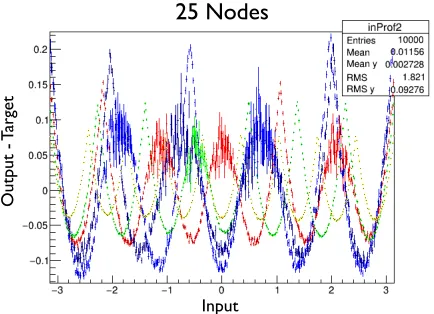
Vector to Vector

2



Zero crossings correspond to

the segments used to

approximate V



Divided among the 3 variables

(not always evenly)



_{Suspect this is from ReLU case}

where all inputs < 0 and

gradient becomes 0.



Initial weights also play a role

25 Nodes

Figure 3.This plot shows the difference between the actual ANN output and the desired output (target)

as a function of the ANN input. The plot is a “profile” histogram meaning they-value of each point rep-resents the average of the difference for all the examples falling in the given input bin of the histogram.

The error bar on the point represents the standard deviation of all the differences associated with that

bin. The different colors represent trials with different randomly initialized weights.

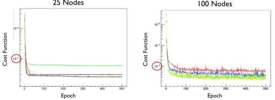
Comparing the performance of different trials of network training (Fig. 4) the most

losing one or two from the equation (for example, because of unlucky initial weight values), is a bigger impediment than when there are many nodes available for the approximation.

Vector to Vector

2

Network performances

25 Nodes

Epoch Epoch

Cost

Function

Cost

Function

100 Nodes

Figure 4. Validation loss for two sets of training trials, one for which the ANN has a single hidden layer with 25 nodes, the other for a single layer ANN with 100 nodes. The different colors represent

trials with different randomly initialized weights.

2.3 Vector to|Vector|2

The final study involves a problem that is quite common in physics: finding the magnitude of a vector. For this study, it is natural to consider two layer ANNs where the two layers in the network serve distinct purposes. It is natural to think of the first layer as calculating the square of each component of the vector, while the second layer is responsible for performing the sum over the three squared components. In this construction, intuitively, one would expect that the second hidden layer should have three nodes, while the number of nodes in the first hidden layer would determine the precision of the approximation of the functionyi=x2_i. See

Fig 5. For this study, an ANN with 500 nodes in the first layer and three in the second is used. Alternatively, the two layer ANN could be constructed with an arbitrary number of nodes in the two hidden layers. After a number of different topologies were explored, one with 251

nodes in each of the two hidden layers was chosen as the alternative model.

Σ y

z x

500 hi

dde

n node

s

x

y

z

x2

y2

z2

|v2_|

251 hi

dde

n

node

s

251 hi

dde

n

node

s

x

y

z

500 hi

dde

n node

s

x

y

z 3 hi

dde

n node

s

|v2_|

+ =

Intuitive

Alternative

Figure 5. Two possible topologies for this ANN. If the “intuitive” approach, the first layer of the network is modeled after thevector to vector2_{network while the second layer is modeled after a simple}

“adder”. In the “alternative” approach, the two hidden layers are chosen to have an arbitrary number of nodes, in this case, 251.

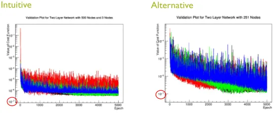
The surprising conclusion of this study is that the alternative ANN structure (two layers each with 251 nodes) tended to do slightly better than the intuitive structure. See Fig. 6 The performance advantage is not large, although it should be noted that there is some evidence in the figure that the alternative topology would have continued to improve with training beyond

losing one or two from the equation (for example, because of unlucky initial weight values), is a bigger impediment than when there are many nodes available for the approximation.

Vector to Vector

2

Network performances

25 Nodes

Epoch Epoch

Cost

Function

Cost

Function

100 Nodes

Figure 4. Validation loss for two sets of training trials, one for which the ANN has a single hidden layer with 25 nodes, the other for a single layer ANN with 100 nodes. The different colors represent

trials with different randomly initialized weights.

2.3 Vector to|Vector|2

The final study involves a problem that is quite common in physics: finding the magnitude of a vector. For this study, it is natural to consider two layer ANNs where the two layers in the network serve distinct purposes. It is natural to think of the first layer as calculating the square of each component of the vector, while the second layer is responsible for performing the sum over the three squared components. In this construction, intuitively, one would expect that the second hidden layer should have three nodes, while the number of nodes in the first hidden layer would determine the precision of the approximation of the functionyi=x2_i. See

Fig 5. For this study, an ANN with 500 nodes in the first layer and three in the second is used. Alternatively, the two layer ANN could be constructed with an arbitrary number of nodes in the two hidden layers. After a number of different topologies were explored, one with 251

nodes in each of the two hidden layers was chosen as the alternative model.

Σ y

z x

500 hi

dde

n node

s

x

y

z

x2

y2

z2

|v2_|

251 hi

dde

n

node

s

251 hi

dde

n

node

s

x

y

z

500 hi

dde

n node

s

x

y

z 3 hi

dde

n node

s

|v2_|

+ =

Intuitive

Alternative

Figure 5. Two possible topologies for this ANN. If the “intuitive” approach, the first layer of the network is modeled after thevector to vector2_{network while the second layer is modeled after a simple}

“adder”. In the “alternative” approach, the two hidden layers are chosen to have an arbitrary number of nodes, in this case, 251.

The surprising conclusion of this study is that the alternative ANN structure (two layers each with 251 nodes) tended to do slightly better than the intuitive structure. See Fig. 6 The performance advantage is not large, although it should be noted that there is some evidence in the figure that the alternative topology would have continued to improve with training beyond

5,000 epochs while the intuitive topology seems to have reached a plateau in validation loss improvement.

Vector to |Vector|

Intuitive Alternative

Figure 6. Validation loss for two sets of training trials, one for which the ANN has an “intuitive” structure as defined in Fig. 5 and one with the “alternative” structure. The different colors represent

trials with different randomly initialized weights.

3 Future Work

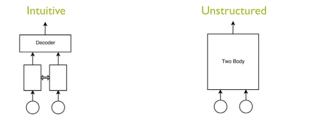
Ultimately, the goal of these studies is to develop intuition for constructing the appropriate ANN topology and size to handle more complicated HEP-related problems. For example, suppose one would like to consider whether two particles (each represented by a momentum vector) result from the decay of some other particle. An ANN can be constructed to try to accomplish this goal. However, it is not clear how best to structure the ANN. Fig. 7 shows two possible different approaches. In the “intuitive” approach each particle momentum

vector is first passed through one more more layers (potentially with shared weights) that just connects the components of single particle momentum vector together before the output of the two individual particle network is combined in a subsequent set of layers. In contrast, the unstructure approach puts the components of both vectors into a set of hidden layers that makes no distinction between the two particles. There are certainly even more topologies that could be explored, and for each topology there are always the questions of how many hidden layers to use and how many nodes should be in each hidden layer. Building an intuition about the best way to structure and size ANNs would help in limiting the size of the hyperparameter space that one must explore to optimize a given network.

4 Conclusions

To realize the potential of DNNs to solve challenging particle physics problems, it is help-ful to develop some intuition about how to large to make the networks and now to select a promising topology. To aid in gaining such intuition, a set of studies were undertaken in-volving relatively simple functions common to basic particle physics problems. The studies revealed the ANNs don’t always learn solutions that one would expect. Furthermore, us-ing a larger number of hidden nodes in a given layer not only improves the accuracy of the ANN approximation, but also helps to sure that multiple different trials of ANN training give

less variation as a function of the different number of random weights. Finally, although

Future Work

Ask questions similar to Vector to |Vector|2_{experiment, but this time}

taking multiple four vectors as inputs.

Intuitive

Unstructured

Figure 7. Two possible ANN topologies for solving a problem involving two particle momentum vectors, indicated by the circles. In the “intuitive” approach, each momentum vector is first passed through its own set of hidden layers. The double-ended open arrow indicates the possibility that the weights of these two sets of layers may be shared. Then the output of the two sets of individual-vector layers is passed into a set of layers that combines information from the two individual-vectors. In the “unstructured” approach, information from both vectors are passed into a single set of hidden layers.

intuition. Additional studies will be required in order to arrive at a point where one can make a well informed choice about the best size or topology for a DNN used to address a complex problem in particle physics.

References

[1] P. Baldi, P. Sadowski, D. Whiteson, Nature Commun.5, 4308 (2014),1402.4735

[2] F. Chollet,Keras, https://github.com/fchollet/keras (2015)

[3] Theano Development Team, arXiv e-printsabs/1605.02688(2016)

[4] D.P. Kingma, J. Ba, CoRRabs/1412.6980(2014),1412.6980

EPJ Web of Conferences 214, 06019 (2019) https://doi.org/10.1051/epjconf/201921406019