— An extended abstract of this work appears in the proceedings of Advances in Cryptology -CRYPTO 2012. This is the full version. —
Differential Privacy with Imperfect Randomness
Yevgeniy Dodis∗ New York University
Adriana L´opez-Alt New York University
Ilya Mironov Microsoft Research Salil Vadhan†
Harvard University August 1, 2012
Abstract
In this work we revisit the question of basing cryptography on imperfect randomness. Bosley and Dodis (TCC’07) showed that if a source of randomness R is “good enough” to generate a secret key capable of encrypting k bits, then one can deterministically extract nearly k almost uniform bits from R, suggesting that traditional privacy notions (namely, indistinguishability of encryption) requires an “extractable” source of randomness. Other, even stronger impossibility results are known for achieving privacy under specific “non-extractable” sources of randomness, such as the γ-Santha-Vazirani (SV) source, where each next bit has fresh entropy, but is allowed to have a small biasγ <1 (possibly depending on prior bits).
We ask whether similar negative results also hold for a more recent notion of privacy called
differential privacy (Dwork et al., TCC’06), concentrating, in particular, on achieving differential privacy with the Santha-Vazirani source. We show that the answer is no. Specifically, we give a differentially private mechanism for approximating arbitrary “low sensitivity” functions that works even with randomness coming from a γ-Santha-Vazirani source, for any γ < 1. This provides a somewhat surprising “separation” between traditional privacy and differential privacy with respect to imperfect randomness.
Interestingly, the design of our mechanism is quite different from the traditional “additive-noise” mechanisms (e.g., Laplace mechanism) successfully utilized to achieve differential privacy with perfect randomness. Indeed, we show thatany(accurate and private) “SV-robust” mechanism for our problem requires a demanding property calledconsistent sampling, which is strictly stronger than differential privacy, and cannot be satisfied by any additive-noise mechanism.
∗Supported by NSF Grants CNS-1065134, CNS-1065288, CNS-1017471, CNS-0831299 and Google Faculty Award. †Supported by NSF grant CCF-1116616 and a gift from Google, Inc. Work done in part while visiting Microsoft
1
Introduction
Most cryptographic algorithms require randomness (for example, to generate their keys, probabilisti-cally encrypt messages, etc.). Usually, one assumes that perfect randomness is available, but in many situations this assumption is problematic, and one has to deal with more realistic, “imperfect” sources of randomness R. Of course, if one can (deterministically) extract nearly perfect randomness from R, then one can easily implement traditional cryptographic schemes with R. Unfortunately, many natural sources are not extractable [SV86,CG88,Zuc96]. The simplest example of such a source is the Santha-Vazirani (SV) source [SV86], which produces an infinite sequence of (possibly correlated) bits
x = x1, x2, . . ., with the property that Pr[xi = 0 |x1. . . xi−1]∈ [12(1−γ),12(1 +γ)], for any setting of the prior bits x1. . . xi−1. Namely, each bit has almost one bit of fresh entropy, but can have a small biasγ <1 (possibly dependent on the prior bits). Yet, the result of Santha and Vazirani [SV86] showed that there exists no deterministic extractorExt:{0,1}n→ {0,1} capable of extracting even a
single bit of biasstrictly less thanγ from the γ-SV source, irrespective of how many SV bitsx1. . . xn
it is willing to wait for. In particular, outputting the first bit is already optimal in terms of traditional extraction.
Despite this pessimistic result, ruling out the “black-box compiler” from perfect to imperfect (e.g., SV) randomness forallapplications, one may still hope that specific “non-extractable” sources, such as SV-sources, might be sufficient forconcreteapplications, such as simulating probabilistic algorithms or cryptography. Indeed, a series of results [VV85,SV86,CG88,Zuc96,ACRT99] showed that very “weak” sources (including SV-sources and much more) are sufficient for simulating probabilistic polynomial-time algorithms; namely, for problems which do not inherently need randomness, but which could potentially be sped up using randomization. Moreover, even in the area of cryptography — where randomness isessential(e.g., for key generation) — it turns out that many “non-extractable” sources (again, including SV sources and more) are sufficient for authentication applications, such as the designs of MACs [MW97,DKRS06] and even signature schemes [DOPS04] (under appropriate hardness assumptions). Intuitively, the reason for the latter “success story” is that authentication applications only require that it is hard for the attacker to completely guess (i.e., “forge”) some long string, so having (min-)entropy in our sourceR should be sufficient to achieve this goal.
Privacy with Imperfect Randomness? In contrast, the situation appears to be much less bright when dealing with privacyapplications, such as encryption, commitment, zero-knowledge, etc. First, McInnes and Pinkas [MP90] showed that unconditionally secure symmetric encryption cannot be based on SV sources, even if one is restricted to encrypting a single bit. This result was subsequently strengthened by Dodis et al. [DOPS04], who showed that SV sources are not sufficient for building even computationally secure encryption (again, even of a single bit), and, if fact, essentially any other cryp-tographic task involving “privacy” (e.g., commitment, zero-knowledge, secret sharing, etc.). Finally, Bosley and Dodis [BD07] showed an even more general result: if a source of randomness Ris “good enough” to generate a secret key capable of encrypting k bits, then one can deterministically extract nearly k almost uniform bits from R, suggesting that traditional privacy requires an “extractable” source of randomness. 1
In this work we ask the question if similar pessimistic conclusions also hold for a more recent, but already very influential variant of privacy called differential privacy (DP), introduced by Dwork et al. [DMNS06], concentrating in particular on achieving differential privacy with the simple Santha-Vazirani source.
Main Question: Is it possible to achieve (non-trivial) differential privacy with SV-sources?
As our main result, we give a positive answer to this question, showing a somewhat surprising “separation” between traditional privacy and differential privacy. But, first, let us examine the above question more closely, gradually explaining the path towards our solution.
Differential Privacy. Differential privacy was introduced for the purposes of allowing the owner of a sensitive database D to securely release some “aggregate statistics” f(D) while protecting the privacy of individual users whose data is in D. Unfortunately, revealing f(D) by itself might violate the privacy of some individual records, especially if the attacker has some partial information about D. Instead, we wish to design arandomized mechanismM(D, f;r) which will approximatef(D) with relatively high accuracy, but will use its randomnessrto “add enough noise” to the true answerf(D) to protect the privacy of the individualrecords of D. For simplicity, we will restrict our attention to real-valued queries f, so that we can define theutility ρ of M as the expected value (over uniform r, for now) of|f(D)−M(D;r)|, which we want to minimize. For example, f might be acounting query, wheref(D) is the number of records inDsatisfying some predicateπ, in which case we seek to achieve utility o(|D|) or even independent of |D|. More interestingly, we wantM to satisfy the following very strong notion called ε-differential privacy: for any neighboring databases D1 and D2 (i.e. D1 and D2 differ on a single record) and for any potential output z, Prr[M(D1, f;r) = z]/Prr[M(D2, f;r) = z]
is between e−ε ≈1−εand eε ≈1 +ε(assuming εis close to 0). This definition shows one difference between standard privacy, which holds between all pairs of databases D1 and D2, and differential privacy, which only holds for neighboring databases. Related to the above, one cannot achieve any useful utility ρ if ε is required to be negligibly small (as then one can gradually transfer any D1 to any other D2 without noticeably changing the answers given by M). Instead, one typically assumes that εis a small constant which can be pushed arbitrarily close to 0, possibly at the expense of worse utility ρ. Motivated by these considerations, we will say thatf admits a class of accurate and private
mechanisms M={Mε |ε > 0} if there exists some fixed function g(·) such that, for allε >0, Mε is
ε-differentially private and has utilityg(ε), independent of the size of the databaseD.
Additive-Noise Mechanisms. The simplest class of accurate and private mechanisms (with per-fect randomness) are the so called additive-noise mechanisms[DMNS06, GRS09, HT10], introduced in the original work of [DN03,DN04,BDMN05,DMNS06]. These mechanisms have the formM(D, f;r) = f(D) +X(r), whereX is an appropriately chosen “noise” distribution added to guarantee ε-DP. For example, for counting queries (and more general “low-sensitivity” queries where |f(D1)−f(D2)| is bounded on all neighboring databases D1 and D2), the right distribution is the Laplace distribution with standard deviation Θ(1/ε) [DMNS06], giving the (additive-noise) Laplace mechanism for such functions, which is private and accurate (in fact, essentially optimal for a wide range of loss func-tions [GRS09]). One perceived advantage of additive-noise mechanisms comes from the fact that the noise is oblivious to the input, and it is natural to ask if it is possible to design additive-noise mechanisms which would be accurate and private even if the noise distribution is generated using the Santha-Vazirani source. For example, perhaps one can generate a “good enough” sample of the Laplace distribution even with SV sources? Unfortunately, we show that this is not the case. In fact, any accurate and private additive-noise mechanism for a source R implies the existence of a randomness extractor for R, essentially collapsing the notion of differential privacy to that of tradi-tional privacy, and showing the impossibility of accurate and private additive-noise mechanisms for SV sources.
Need for Consistent Sampling. In fact, the main reason why additive-noise mechanisms fail to handle SV sources comes from the fact that such algorithms usedisjoint setsof coins to produce the same “noisy answer” on two databases having different “real answers”. More formally, if f(D1) 6= f(D2) andTi(z) is the set of coinsrwhereM(Di, f;r) =z, an additive-noise mechanism must satisfy
T2(z)] ≤ 1 +ε. For the uniform distribution, this simply means that |T1| ≈ |T2|. Since T1 and T2 are disjoint, the SV adversary can try to bias the coinsrso as to simultaneously increase (or, at least maintain) the odds of hitting T1, while decreasing the odds of hitting T2. Indeed, in Lemma 2.4 we show that an SV adversary can always succeed in amplifying the ratio Prr[r∈T1]/Prr[r∈T2] (and,
hence, violate the differential privacy of our mechanism) whenever T1 and T2 have small intersection (e.g., are disjoint).
In fact, in Lemma 3.2 we prove that any “SV-robust” mechanism should strive to produce iden-tical outputs on neighboring databases for a majority of random tapes; in particular, for any z, |T1(z)∩T2(z)| ≈ |T1(z)| ≈ |T2(z)| (see Definition 4.1 for the exact quantitative formulation). This general property, which we call consistent sampling (CS), is closely related to the “consistent sam-pling” methodology that has found applications in web search [BGMZ97] and parallel repetition the-orems [Hol07], among others. Moreover, we show that ε-consistent sampling implies ε-differential privacy, but the converse is false.
Our Main Result. The lower bound above suggests a path forward toward building SV-robust mechanisms, which starts with the design of consistently samplable mechanisms. For example, the classical Laplace mechanism for low sensitivity functions could be viewed as sampling some noise x of expected magnitude ρ = O(1/ε), and adding it to the exact solution y = f(D). Being additive-noise, this mechanism is not CS. But, imagine a new mechanism which further rounds the answer z =y+x to the nearest multiple z′ of 1/ε. Clearly, the expected utility has gone from ρ to at most ρ′ =ρ+ 1/ε = O(ρ). Yet, it turns out that the new mechanism is now ε-CS, since, informally, the
roundedanswers on neighboring databases are only distinct on anε-fraction of coinsr(see Section 5). Still, designing CS mechanisms was only anecessarycondition for building SV-robust, differentially private mechanisms. For example, the basic notion of consistency ignores the binary representations of random coinsrdefining the needed pre-image setsT1 andT2, which are (intuitively) very important for handling SV sources since their randomness properties are bit-by-bit. Indeed, we show that consistency alone isnotenough for SV-robustness, and we need an additional (fortunately, simply stated) property of our sampling to guarantee the latter. (As expected, this property asks something quite natural about the binary representations of the coins inside T1 and T2.) We call the resulting notionSV-consistent
sampling(SVCS; Definition 4.3). Building an accurate and private mechanism satisfying this condition formed the main technical bulk of our work.
In particular, starting with the “rounded” Laplace mechanism, we show a careful implementation of this CS mechanism, so that the resulting mechanism is actually SVCS (with appropriate parameters guaranteeing ε-DP of the final mechanism against γ-SV sources). The details of this technical step, which uses properties of arithmetic coding (see [MNW98, WNC87]) applied to the specific Laplace distribution, are explained in Section 5. This gives us our main result (Theorem 5.3) and an affirmative answer to our Main Question: an accurate and private class of SV-robust mechanisms for counting queries and arbitrary low-sensitivity functions.
To maintain a clear presentation, we defer more technical proofs to Appendix A.
2
Random Sources and Differential Privacy
Notation. For a positive integer n, we use the notation [n] to denote the set{1,2, . . . , n}. We use ⌊·⌉to denote the nearest integer function. For a distribution or random variableR, we writer ←Rto denote the operation of sampling a random r according to R. For a randomized function h, we write h(x ;r) to denote the unique output of f on inputx with random coins r. When the distribution of random coinsRis understood from context, we write h(x) to denote the random variable h(x ;r) for r ←R. Finally, we denote a sequence of bits using boldface, e.g. x=x1, x2, . . .
continuously outputting (possibly correlated) bits. In particular, we let U be the distribution over {0,1}∗ that samples each bit independently and uniformly at random. When U is truncated after n
bits, the result is the distributionUn, which is the uniform distribution over {0,1}n, the bit-strings of
length n.
2.1 Random Sources
We call a familyRof distributions over{0,1}∗asource. We will sometimes abuse this terminology and
also refer to a single (unknown) distributionRas a source as well (in fact, the latter is the standard use of the termsourcein the randomness extraction literature). In this work, we model perfect randomness with the uniform source and imperfect randomness with γ-Santha-Vazirani sources [SV86], arguably the simplest type of “non-extractable” sources. Theuniform source U def= {U}is the set containing only the distributionUon{0,1}∗ that samples each bit uniformly at random. We defineγ-Santha-Vazirani
sources below.
Definition 2.1 (γ-Santha-Vazirani Source [SV86]). Let γ ∈ [0,1]. A probability distribution X = (X1,X2, . . .)over{0,1}∗ is a γ-Santha-Vazirani distributionif for alli∈Z+andx1. . . xi−1 ∈ {0,1}i−1,
it holds that
1
2(1−γ)≤Pr[Xi= 0|X1 =x1, . . .Xi−1=xi−1]≤ 1
2(1 +γ).
We define the γ-Santha-Vazirani source SV(γ) to be the set of all γ-Santha-Vazirani distributions. Finally, for a distribution SV(γ) ∈ SV(γ), we let SV(γ, n) be the distribution SV(γ) restricted to the first n coins (X1, . . . ,Xn). We let SV(γ, n) be the set of all distributions SV(γ, n).
We now defineγ-biased semi-flat sources, which were introduced by [RVW04] (see also [DOPS04], where they were referred to as γ-biased halfspace sources).
Definition 2.2 (γ-Biased Semi-Flat Source). For S ⊂ {0,1}n of size |S|= 2n−1, and γ ∈[0,1], the
distribution HS(γ, n) over {0,1}n is defined as follows: for all x∈S, Prx←HS(γ,n)[x] = (1 +γ)·2−n,
and for all x /∈S, Prx←HS(γ,n)[x] = (1−γ)·2−n. We define the γ-biased semi-flat source H(γ, n) to
be the set of all distributions HS(γ, n) for all|S|= 2n−1.
Lemma 2.3 ([RVW04, DOPS04]). For any n∈Z+ and γ ∈[0,1], H(γ, n)⊂ SV(γ, n).
We prove a general lemma about γ-biased semi-flat sources, which will be very useful in later sections.
Lemma 2.4. Let G, B ⊆ {0,1}n such that |G| ≥ |B| > 0, and let σ def= |B\G|
|B| ∈ [0,1]. Then there
exists S⊆ {0,1}n of size |S|= 2n−1 such that Prr←HS(γ,n)[r∈G]
Prr←HS(γ,n)[r∈B]
≥(1 +γσ)·|G| |B|.
Proof. Let G′ def= G\B, B′ def= B\G, and N def= G∩B. Let α def= |G′|, β def= |B′|, and λ def= |N|. We
consider two cases: 1. α≤2n−1, and 2. α >2n−1
Case 1: First suppose that α ≤2n−1, which means also β ≤2n−1 since we assume |G| ≥ |B|. Then pick anyS ⊂ {0,1}n of size|S|= 2n−1 such thatG′⊆S andB′∩S =∅. Letλ0
def
λ1
def
= λ−λ0. Then
Prx←HS(γ,n)[x∈G] Prx←HS(γ,n)[x∈B]
= (1 +γ)α+ (1 +γ)λ0+ (1−γ)λ1 (1−γ)β+ (1 +γ)λ0+ (1−γ)λ1 ≥ (1 +(1 γ)α+ (1 +γ)λ
−γ)β+ (1 +γ)λ
= α+λ β+λ
β+λ
1−γ
1+γ β+λ = α+λ β+λ· 1
∆, (2.1)
where ∆def=
“ 1−γ 1+γ
”
β+λ
β+λ . We have,
∆ =
1−γ
1+γ
β+λ β+λ = 1−
2γ
1+γ
β β+λ = 1−
2γσ 1 +γ =
1 +γ−2γσ 1 +γ . Then, plugging in this value of ∆ in (2.1), we have
Prx←HS(γ,n)[x∈G] Prx←HS(γ,n)[x∈B]≥
α+λ β+λ
1 +γ 1 +γ−2γσ
= α+λ β+λ
1 + 2γσ 1 +γ−2γσ
≥ α+λ
β+λ(1 +γσ), where the last inequality follows from σ <1.
Case 2: Now assume that α >2n−1. Then pick anyS ⊂ {0,1}n of size|S|= 2n−1 such thatS ⊆G′.
Letα0 def= |S∩G′|= 2n−1 andα1def= α−α0. Then Prx←HS(γ,n)[x∈G]
Prx←HS(γ,n)[x∈B]
= (1 +γ)α0+ (1−γ)α1+ (1−γ)λ (1−γ)β+ (1−γ)λ
=
1+γ
1−γ
α0+α1+λ β+λ =
α0+α1+λ β+λ +
2γ
1−γ
α0 β+λ ≥ α0+α1+λ
β+λ
1 +
2γ 1−γ
1 2 = α+λ β+λ
1 + γ 1−γ
≥ α+λ
β+λ·(1 +γ) ≥ αβ++λλ·(1 +σγ).
2.2 Differential Privacy and Utility
The Model. We model a statistical database as an array of rows from some countable set, and say that two databases areneighboring if they differ in exactly one row. Throughout the paper, we letD be the space of all databases. We consider the interactive setting, in which interested parties submit queries, modeled as functions f :D → Z, where Z is a specified range. In this paper, we are only concerned with queries with rangeZ =Z, and henceforth only consider this case. Amechanism M is a probabilistic algorithm that takes as input a database D∈ D and a queryf :D →Z, and outputs a value z ∈Z. We assume that M’s random tape is in{0,1}∗, that is, thatM has at its disposal a possibly infinite number of random bits, but for a fixed outcomez∈Z,M needs only a finite number of coinsn=n(D, f, z) to determine whetherM(D, f) =z. Furthermore, we assume that ifr∈ {0,1}n
is a prefix of r′ ∈ {0,1}n′ and M(D, f ;r) = z is already determined from r, then M(D, f ;r′) = z also. In other words, providing M with extra coins does not change its output.
Definitions. Informally, we wish z = M(D, f) to approximate the true answer f(D) without re-vealing too much information. We say a mechanism is differentially privatefor a class F of queries if for all queriesf ∈ F, replacing a real entry in the database with one containing fake information only changes the output distribution of the mechanism by a small amount. In other words, evaluating the mechanism on the same query f ∈ F, on two neighboring databases, does not change the outcome distribution by much. On the other hand, we define its utility to be the expected difference between the true answerf(D) and the output of the mechanism. Since the purpose of this work is to analyze mechanisms with respect to their sources of randomness, the following definitions of privacy and utility explicitly take the source of randomness Rinto account.
Definition 2.5 ((ε,R)-Differential Privacy). Let ε ≥0, R be a source, and F = {f :D → Z} be a class of functions. A mechanism M is (ε,R)-differentially private for F if for any pair D1, D2 ∈ D
of neighboring databases, all f ∈ F, all possible outputs z∈Z of M, and all R∈ R:
Prr←R[M(D1, f ;r) =z]
Prr←R[M(D2, f ;r) =z]
≤1 +ε.
This is a very strong definition. Not only does it give astatistical guarantee, making it independent of the computation power of any adversary, but it is also strictly stronger than the requirement that the statistical distance between M(D1, f) and M(D2, f) is at mostε (for example, the latter allows some low-probability outcomes of M(D1, f) to never occur under M(D2, f)). We also note that, traditionally, differential privacy has been defined by having the ratio of probabilities be bounded by eε. We instead bound it by 1+ε, since this formulation makes some of our calculations slightly cleaner. This is fine since we always have 1 +ε≤eε, and, whenε∈[0,1] (which is the main range of interest), we anyway have eε ≈1 +ε.
If a mechanismM is (ε,R)-differentially private for some randomness sourceR, then a mechanism M′ that runs M as a black box and then performs some post-processing on the output, is also (ε,R )-differentially private. Intuitively, this is because given only z = M(D, f), M′ cannot reveal more
information about D than z itself. In our work we only consider the case where M′ evaluates a
deterministic functionh of z=M(D, f), so that M andh do not have to “share” the random source R.
Lemma 2.6. Let M be a (ε,R)-differentially private mechanism, and let h be any function. Define
M′(D, f)def= h(M(D, f)). Then M′ is (ε,R)-differentially private.
Definition 2.7 ((ρ,R)-Utility). Let ρ > 0, let R be a source, and let F = {f : D → Z} be a class of functions. We say a mechanism M has (ρ,R)-utility for F if for all databases D∈ D, all queries
f ∈ F, and all distributions R∈ R,
For example, in the case whereF is the class of counting queries, where f ∈ F is the number of records inD satisfying some predicateπ, we seek to achieve utilityρ=o(|D|) or even independent of |D|.
At the extremes, a mechanism that always outputs 0 is (0,R)-differentially private, while a mech-anism that outputs the true answer f(D) has (0,R)-utility. Neither of these mechanisms is very interesting—the first gives no utility, while the second provides no privacy. Instead, we wish to find mechanisms that achieve a good trade-off between privacy and utility. This motivates the following definition.
Definition 2.8 (Accurate and Private Mechanisms). We say a function family F admits accurate and private mechanisms w.r.t. R if there exists a function g(·) such that for all ε > 0 there exists a mechanism Mε that is (ε,R)-differentially private and has (g(ε),R)-utility. We call M={Mε} a
class of accurate and private mechanisms for F w.r.t. R.
We make a few remarks regarding this definition. First, we require that the utility ρ = g(ε) is independent of |D|. Second, we note that satisfying this definition implies that we can achieve (ε,R )-differential privacy for any ε > 0 (possibly at the expense of utility). E.g., when R = SV(γ), we should be able to achieve ε≪ γ, which is below the “extraction barrier” for SV-sources. Finally, we note that for the purpose of satisfying this definition, we can assume w.l.o.g. that ε ≤ 1, which is anyway the case of most interest. Moreover, we can assume that 1/εis an integer, since otherwise we can simply take a slightly smaller εfor which this is the case.
Infinite-Precision Mechanisms. As we will see shortly, it is sometimes easier to describe mech-anisms using samples from some continuous random variable X, instead of using a (discrete) random tape in {0,1}∗. Moreover, the notions of privacy and utility can be analogously defined for this case as well (which we omit for brevity). Of course, to actually “implement” such abstract mechanisms in practice, one must specify how to approximate them using a “finite precision” random tape in{0,1}∗,
without significantly affecting their privacy and/or utility. When perfect randomness U is available, this is typically quite easy (and usually not spelled out in most differential privacy papers), by simply approximating a continuous sample from X within some “good enough” finite precision (see [Mir12] for a detailed exposition of how this can be achieved). In contrast, our mechanisms will have to deal with imperfect randomness SV(γ), so rounding a given “continuous” mechanism into a “discrete” mechanism will be non-trivial and require utmost care. In particular, we will have to design quite spe-cial “infinite-precision” mechanisms which will be “SV-friendly” toward appropriate “finite-precision rounding”.
Additive Noise Mechanisms. One type of accurate and private mechanisms follow the following blueprint: first, they sample data-independentnoisexfrom some (discrete or continuous) distribution
X, calculate the true answerf(D), and outputz=f(D) +x. We call such mechanisms,additive-noise
mechanisms (examples of additive-noise mechanisms include the Laplacian mechanism [DMNS06],
the geometric mechanism [GRS09], and theK-norm mechanism for multiple linear queries [HT10]). If
E[|X|] is bounded, then the mechanism has good utility. However, to argue that such bounded “noise”
X is sufficient to ensure the differential privacy of such mechanisms, we must first restrict our query class F. In particular, it turns out that additive-noise mechanisms achieve differential privacy for a pretty large class of useful functions, called bounded sensitivityfunctions.
Definition 2.9 (Sensitivity). Forf :D →Z, the sensitivity of f is defined as
∆f def= max
D1,D2k
f(D1)−f(D2)k
for all neighboring databases D1, D2 ∈ D. For d∈Z+, we define Fd ={f :D → Z|∆f ≤d} to be
As an example, counting queries are inF1. Intuitively, low sensitivity functions do not change too much on neighboring databases, which suggests that relatively small noise can “mask” the difference between f(D1) and f(D2). The particular (continuous) distribution turns out to be the Laplacian distribution, defined below.
Definition 2.10 (Laplacian Distribution). The Laplacian distribution with mean µ and standard deviation √2b, denoted Lapµ,b, has probability density function Lapµ,b(x) = (1/2b) ·e−|x−µ|/b. The cumulative distribution function is CDFLapµ,b(x) = (1/2b)·(1 + sgn(x)·(1−e|x−µ|/b)).
We also define the distribution obtained from sampling the Laplacian distributionLapµ,band round-ing to the nearest integer ⌊Lapµ,b⌉. We call this the “rounded” Laplacian distribution and denote it by
RLapµ,b.
In particular, for any sensitivity bound d, Dwork et al. [DMNS06] showed that the following class of (infinite-precision) additive-noise mechanismsMLap={MLap
ε } is accurate and private forFd.
Given a database D ∈ D, a query f ∈ Fd and the target value of ε, the mechanism MεLap computes
f(D) and adds noise from the Laplacian distribution with mean 0 and standard deviation (√2·d)/ε; i.e. MεLap(D, f) def= f(D) +Lap0,d/ε. Equivalently, we can also view this mechanism as computing
y=f(D) and outputting a sample from the distributionLapy,d/ε. Moreover, it is easy to see that this infinite-precision mechanism achieves O(d/ε)-utility.
In order to ensure that the output of the mechanism of [DMNS06] is an integer, the result can be rounded to the nearest integer. Since this is post-processing, by Lemma 2.6, the result has the same privacy guarantees. Furthermore, since f(D) ∈Z, we have ⌊f(D) +Lap0,d/ε⌉ =y+⌊Lap0,d/ε⌉. In particular, for queries of integer range, the mechanism of [DMNS06] can be seen as computing y = f(D) and outputting z = RLapy,d/ε. We denote this (still infinite-precision, but now integer range) variant byMεRLap. Clearly, it still has utilityO(d/ε).
Finally, we must describe how to approximate this mechanism family MRLap by a finite precision
family MRLap w.r.t. U, without significantly affecting privacy or utility. As it turns out, a good enough approximation can be accomplished by sampling each value z ∈ Z with precision roughly proportional to Pr[z] (under MεRLap), which requires n(z) = O(|z|log(d/ε)) (truly random) coins Un(z), and increases both ε and ρ by at most a constant factor. Since we will not use the resulting (finite-precision) mechanism in this paper2, we state the end result without further justification.
Lemma 2.11 ([DMNS06]). For any d∈Z+, there exists a familyMRLap={MRLapε } of accurate and private mechanisms for Fd w.r.t. the uniform source U, with utility function gRLap(ε) =O(d/ε).
Our Question. Lemma 2.11 shows that for all d∈Z+ there exists a class of accurate and private mechanisms for Fd w.r.t. U. The main goal of this work is to determine if this is also true for other
randomness sources, in particular, for the γ-Santha-Vazirani sources.
Main Question (Restated): Does there exist a classM={Mε} of accurate and private
mecha-nisms for Fdw.r.t. SV(γ) for all γ ∈[0,1)? If so, can they be additive-noise mechanisms?
For clarity, from now we will focus on the cased= 1; however, all our results extend to any sensitivity bound d (with utility scaled by a factor of d). We will prove that accurate and private mechanisms forF1 w.r.t. SV(γ) cannot be additive noise, answering the second question in the negative. Despite this, however, we will answer the first question positively by displaying a classM={Mε}of accurate
and private (non-additive-noise) mechanisms for F1 w.r.t. SV(γ).
3
Naive Approaches and a Lower Bound
We will start by showing a few naive approaches that will explain the intuition behind why accurate and private mechanisms for F1 w.r.t. SV(γ) cannot be additive noise. Moreover, we will prove a general lower bound restricting the type of mechanisms “friendly” to SV-sources, which will motivate a very special type of mechanisms that we will introduce in Section 4.
First Attempt. A first approach to answer our main question would be to prove that any class of accurate and private mechanisms forF1 w.r.t.U is also accurate and private w.r.t.SV(γ). This turns out to be far too optimistic. To see this, take any mechanism M w.r.t. U, and assume that with high probability M needs at mostnrandom coins. Define (artificial) mechanismM′ as follows. Whenever M needs a fresh coin bi, M′ samplesk coins bi1. . . bik and simply setsbi =majk(bi1, . . . , bik), where
majk(·) is the majority of kbits. Clearly,M′ has the same differential privacy and utility guarantees
as M w.r.t. U, since majority of perfectly random bits is perfectly random. On the other hand, by biasing each bit towards 0 (resp. 1), a Santha-Vazirani adversary can fix each k-bit majority function to 0 (resp. 1) with probability at least (1−e−γ2k/2
), which means that he can fix all n coins of M to any desired outcome with probability at least (1−ne−γ2k/2) ≈1 for k=O(logn/γ2). Hence, the Santha-Vazirani adversary for M′ can effectively fix the random tape of M, making it deterministic (with probability arbitrarily close to 1). On the other hand, it is easy to see that no deterministic mechanism having non-trivial utility (i.e., giving distinct answers on some two neighboring databases) can be differentially private.
Hence, accurate and private mechanisms w.r.t. the uniform sourceU are not necessarily accurate and private w.r.t. γ-Santha-Vazirani sources SV(γ).
Second Attempt. A seemingly less naive idea would be to prove that any class of accurate and private mechanisms for F1 w.r.t. U is also accurate and private w.r.t. SV(γ) if we first run some randomness extractor Ext on the randomness. More precisely, suppose M = {Mε} is accurate and
private w.r.t. U and suppose Mε uses n coins. Can we construct a deterministic extractor Ext :
{0,1}m → {0,1}n (for some sufficiently large m ≫ n) and let M′
ε
def
= Mε(D, f ;Ext(r)), such that
M′ ={M′
ε}is accurate and private w.r.t.SV(γ)wheneverM={Mε}is accurate and private w.r.t.U?
More generally, one can define an analogous “extractor conjecture” for any imperfect sourceRin place of SV(γ). Unfortunately, we show that this naive approach does not work for any “non-extractable” source R, such as SV(γ). To show this, we look at the family of additive-noise mechanisms for the family F1 of sensitivity-1 functions given by Lemma 2.11, and observe that applying an extractor to any additive-noise mechanism is still an additive-noise mechanism. Then, we show a more general statement thatanyaccurate and private additive-noise mechanism forF1underRimplies the existence of a bit extractor for R, which is impossible for non-extractable R, such asSV(γ).
Lemma 3.1. AssumeR is a source and M={Mε} is a family ofadditive-noisemechanisms for F1,
where each Mε is (ε,R)-differentially private. Then, for all ε >0, one can deterministically extract
an ε-biased bit from R. In particular, there does notexist a class M={Mε}of accurate and private
additive-noise mechanisms for F1 w.r.t. any “non-extractable” R, such as SV(γ).
Proof. Given any class M = {Mε} of additive-noise mechanisms for F1, define a new class M′ =
{Mε′} of binary-output mechanisms, where Mε′(D, f;r) =Mε(D, f;r) mod 2. Notice, if Mε is (ε,R
)-differentially private, then so is M′
ε by Lemma 2.6 (since mod 2 is a deterministic post-processing
function). Also, sinceMεis additive-noise, we can writeMε(D, f;r) =f(D)+x, wherex=Extε(r) for
some functionExtε:{0,1}∗ →Z. Thus, if we let Ext′ε(r) =Extε(r) mod 2, we can writeMε′(D, f;r) = (f(D) mod 2)⊕Ext′ε(r), where ⊕is the exclusive-or operator on one bit.
thatMε′(Db, f;r) = (f(Db) mod 2)⊕Extε′(r) =b⊕Ext′ε(r). By (ε,R)-differential privacy ofMε′ applied
to D0 and D1, this means that for any R∈ R, we must have Pr[Ext′ε(R) = 0] ∈[12(1−ε),12(1 +ε)], which would mean that Ext′ε defines an ε-biased one-bit extractor for R.
General Lower Bound. The failure of our naive approaches suggests that one cannot take any accurate and private mechanism w.r.t. uniform randomnessU, and apply some simple transformation to its randomness to derive an accurate and private mechanism w.r.t. SV(γ). Indeed, we will show thatanyaccurate and private mechanism w.r.t.SV(γ) must in fact satisfy a fairly restrictive condition with respect to the uniform source. In particular, this condition (later called consistent-sampling) is never satisfied by additive-noise mechanisms.
First, we need some important notation. Consider a mechanismM with randomness space{0,1}∗,
and let D ∈ D. We define the set T(D, f, z) def= {r ∈ {0,1}n | z = M(D, f ;r)} to be the set of random coinsr∈ {0,1}∗ such that M outputszwhen run on databaseD, queryf, and random coins
r. We remark that since we assume that onlyn=n(f, z, D) coins need to be sampled to determine if M(D, f) =z, we can assume w.l.o.g. that T(f, z, D) ⊆ {0,1}n. In the interest of clarity, we simply write T when f, D, and z are understood from context.
Without loss of generality, we assume that the function familyF is by itself non-trivial, meaning that there exist two neighboring databases D1, D2 and a query f such that f(D1) 6= f(D2). Fix z ∈ Z, f ∈ F,R ∈ R, and let T1
def
= T(D1, f, z) and T2
def
= T(D2, f, z). To show that M is (ε,R )-differentially private forF w.r.t. randomness sourceR, we are concerned with bounding the following ratio by 1 +ε:
Prr←R[M(D1, f ;r) =z]
Prr←R[M(D2, f ;r) =z]
= Prr←R[r∈T1]
Prr←R[r∈T2]
As we show below, bounding the above ratio for all Santha-Vazirani sources introduces a non-trivial constraint on M. For illustration, let us first look at any additive-noise mechanism M and re-derive the conclusion of Lemma 3.1 directly. If z = M(D1, f ;r1) = M(D2, f ;r2) then z = f(D1) +x1 = f(D2) +x2 forx1, x2 ←X. Since we assumedf(D1)6=f(D2) thenx16=x2, which means thatr16=r2. Thus,T1∩T2=∅. Furthermore, we can assume w.l.o.g. that|T1| ≥ |T2|since otherwise we can switch D1 andD2. Using Lemma 2.4 withG=T1 andB =T2, takingn= max(n(f, z, D1), n(f, z, D2)), and using the fact that H(γ, n)⊂ SV(γ, n), we have that there exists SV(γ)∈ SV(γ) such that
Prr←SV(γ)[M(D1, f ;r) =z]
Prr←SV(γ)[M(D2, f ;r) =z]
≥(1 +γ)·|T1| |T2| ≥
1 +γ,
which is the same conclusion as the one obtained in the proof of Lemma 3.1.
More generally, coming back to arbitrary mechanisms, since Lemma 2.4 works even whenG∩B 6=∅, we get the following much stronger result. Suppose σ def= |T2\T1|/|T2| ∈ [0,1]. Then there exists
SV(γ)∈ SV(γ) such that
Prr←SV(γ)[M(D1, f ;r) =z]
Prr←SV(γ)[M(D2, f ;r) =z]
≥1 +γσ.
This shows that anecessarycondition to achieve (ε,SV(γ))-differential privacy is thatσ ≤ε/γ =O(ε). We summarize this in the following lemma.
Lemma 3.2. Assume γ > 0 and M is (ε,SV(γ))-differentially private mechanism for some class
0 1
T1 T2
Figure 4.1: Example of how a SV(γ)∈ SV(γ) distribution can increase the ratio Prr←SV(γ)[r∈T1]
Prr←SV(γ)[r∈T2].
4
SV-Consistent Sampling
Recall that we defined T(D, f, z) def= {r ∈ {0,1}n | z = M(D, f ;r)} to be the set of all coins r
such that M outputsz when run on database D, query f and randomness r. Further recall that for neighboring databases D1, D2, we letT1 def= T(D1, f, z) andT2 def= T(D2, f, z).
By Lemma 3.2 we know that in order to achieve (ε,SV(γ))-differential privacy we must have |T2\T1|/|T2| = O(ε). This means that as ε → 0, it must be that |T2\T1|/|T2| → 0. This motivates our definition ofεe-consistent sampling. Later we will defineεin terms ofεesuch thatε→0 as εe→0. We remark that our definition of εe-consistent sampling is similar to the definition of [Man94, Hol07], which has already been used in the context of differential privacy for different purposes [MMP+10].
Definition 4.1. We say M has εe-consistent sampling (εe-CS) if for all z∈Z, f ∈ F and neighboring databases D1, D2 ∈ D which define T1, T2 as above, provided T26=∅, we have
|T1\T2| |T2| ≤e
ε.
We make a few remarks about Definition 4.1. First, notice that w.l.o.g. we can assume that |T1| ≥ |T2| since in this case we have |T|2T\1T|1| ≤ |T|1T\2T|2|. Second, notice that εe-consistent sampling also guarantees that |T2\T1|
|T2| ≤ |T1\T2|
|T2| ≤eε, which Lemma 3.2 tells us is a necessary condition for non-trivial differential privacy underSV(γ). Finally, it is easy to see that if a mechanism hasεe-consistent sampling, then it is (ε,eU)-differentially private, as
Prr←Un[r∈T1] Prr←Un[r∈T2]
= |T1| |T2|
= |T1∩T2| |T2|
+|T1\T2| |T2| ≤
1 +ε.e
To summarize,eε-consistent sampling issufficient to achieve (ε,eU)-differential privacy and is essen-tiallynecessary to achieve (γε,eSV(γ))-differential privacy. But is it sufficient to achieve (p(εe),SV(γ ))-differential privacy for some function p such that p(eε) → 0 as εe→ 0? This turns out not to be the case, as it is still possible for a Santha-Vazirani distribution to increase the probability ofT1\T2 while simultaneously decreasing the probability of T2. For instance, consider the example in Figure 4.1, where pictorially, we view each coin r ∈ {0,1}∗ as defining a path down a binary tree. In this
ex-ample, T1\T2 and T2 are positioned precisely to the left and right of 1/2, respectively. After the first coin, the SV-distribution can focus on either targetingT1\T2 or avoidingT2. If T1 andT2 only contain a small fraction of the leaves of this tree, then the SV distribution can greatly increase the ratio of probabilities Prr←SV(γ)[r∈T1\T2]/Prr←SV(γ)[r∈T2]. This suggests that in order to handleγ-Santha
Vazirani distributions, we need to make more restrictions on the mechanism.
x =x1, . . . , xm ∈ {0,1}m, we definesuffix(x)
def
= {y =y1, y2, . . . ∈ {0,1}∗ |xi = yi for all i ∈[m]}
to be the set of all bit strings that have x as a prefix. For n ∈ Z+ such that m ≤ n, we define
suffix(x, n)def= suffix(x)∩ {0,1}n.
Our first observation is that if we consider the longest prefixuof all elements in T1∪T2, then the ratio Prr←SV(γ)[r ∈ T1\T2]/Prr←SV(γ)[r ∈ T2] is the same as when the probabilities are conditioned
on r having this prefix. This is because in order for r ∈ T1\T2 or r ∈ T2, it must be the case that
r∈suffix(u, n).
Our second observation is that we want to ensure that suffix(u, n) is a good approximation of T1∪T2, that is, that |suffix(u, n)| ≈ |T1∪T2|. This guarantees that we never encounter the problem that arose in the example in Figure 4.1. For this to be the case, however, we must first ensure that T1∪T2 are “close together”. We therefore make the following definition.
Definition 4.2. We say M is an interval mechanism if for all queries f ∈ F, databases D ∈ D, and possible outcomes z ∈Z, the values in T = T(D, f, z) constitute an interval, that is, T 6=∅ and the set {int(r) | r ∈ T} contains consecutive integers, where for r = r1. . . rn ∈ {0,1}n, we define
int(r)def= Pni=1ri·2n−i.
We now formalize the requirement we described above. LetD1, D2 be two neighboring databases, let f ∈ F, let z be a possible outcome, letndef= max(n(D1, f, z), n(D2, f, z)), and letT1=T(D1, f, z) and T2=T(D2, f, z). We letu be the longest prefix such thatT1∪T2⊆suffix(u, n). Formally,
udef= argmax{|u′| |u′ ∈ {0,1}≤n and T1∪T2 ⊆suffix(u′, n)}
Definition 4.3. Let ε >e 0, c > 1. We say that an interval mechanism M has (ε, ce )-SV-consistent sampling ((ε, ce )-SVCS) if it has εe-consistent sampling and for all queries f ∈ F, all neighboring databases D1, D2 ∈ D and all possible outcomes z∈Z, which define T1, T2,u as above, we have:
|suffix(u, n)| |T1∪T2| ≤
c
We now show that (ε, ce )-SV-consistent sampling is sufficient to obtain (ε,SV(γ))-differential privacy for an interesting value of ε, that is, for anεthat can be made arbitrarily small by decreasingεe.
Theorem 4.4. If M has (ε, ce )-SV-consistent sampling, then M is (ε,SV(γ))-differentially private, where
ε= 2·(8eε)1+log(1/(1+γ))
1 +γ 1−γ
log(8c)
In particular, for γ∈[0,1) and c=O(1), we have ε→0 as eε→0.
Before proving Theorem 4.4, we make a few additional definitions and prove a lemma. LetD1, D2 be two neighboring databases, f ∈ F,zbe a possible outcome, n= max(n(D1, f, z), n(D2, f, z)), and T1=T(D1, f, z) and T2 =T(D2, f, z).
• Define vto be the longest prefix such that T1\T2 ⊆suffix(v, n). Formally,
v= argmax{|v′| |v∈ {0,1}≤n and T1\T2 ⊆suffix(v′, n)}
• Define I0
def
= suffix(v0, n)∩T1\T2 and I1
def
= suffix(v1, n)∩T1\T2. That is, I0∪I1 =T1\T2 and Ib contains all coins in T1\T2 that havevb as prefix.
– Define v0 to be the longest prefix such that I0⊆suffix(v0, n). Formally,
| {z }
T1| {zT2 }
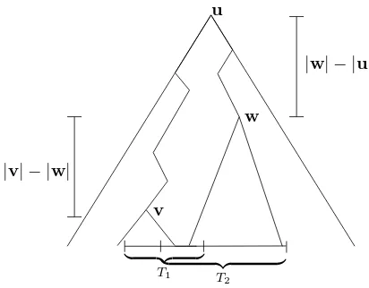
u
v
w
|w| − |u|
|v| − |w|
Figure 4.2: Definitions of u,v,w.
– Define v1 to be the longest prefix such that I1⊆suffix(v1, n). Formally,
v1 = argmax{|v′1| |v1 ∈ {0,1}≤n and I1 ⊆suffix(v1′, n)} • Define wto be a shortest prefix such thatsuffix(w, n)⊆T2. Formally,
w= argmin{|w′| |w′∈ {0,1}≤n andsuffix(w′, n)⊆T2}
We remark thatw may not be unique. In this case, any of the (at most two) possible values is just as good since we will be concerned with the value|w|which is the same across all possible values of w.
See Figure 4.2 for a pictorial representation ofu,v,w. Note the asymmetry of the definitions of
u,v, and w. Also note that we define v and w in such a way that suffix(v)∩suffix(w) = ∅. Informally, min(|v0|,|v1|)− |w| is roughly the number of coins that the Santha-Vazirani distribution needs to use to increase the probability of landing inT1\T2 without affecting the probability of landing inT2, while|w|−|u|is roughly the number of coins that it can use to decrease the probability of landing in T2 without affecting the probability of landing in T1\T2. We first prove a lemma that says that if M has (ε, ce )-SV-consistent sampling then min(|v0|,|v1|)− |w|= Ω(log(1/εe)) and|w| − |u|=O(logc).
Lemma 4.5. If M has (ε, ce )-SV-consistent sampling then for all neighboring databases D1, D2 ∈ D
which define u,v0,v1,w as above, we have:
min(|v0|,|v1|)− |w| ≥log
1 8eε
and |w| − |u| ≤log(8c)
Proof. By (eε, c)-SV-consistent sampling we know that |T1\T2|
|T2| ≤e
ε and |suffix(u, n)| |T1∪T2| ≤
c
We therefore have,
|suffix(v0, n)|/2 +|suffix(v1, n)|/2≤ |I0|+|I1|=|T1\T2| ≤eε· |T2| ≤4εe· |suffix(w, n)|
Reorganizing yields the first inequality. We also have,
|suffix(u, n)| ≤c· |T1∪T2| ≤c·(|T1\T2|+|T2|)≤(1 +εe)·c· |T2| ≤2c· |T2| ≤8c· |suffix(w, n)| n− |u| ≤log(8c) +n− |w|
Reorganizing yields the second inequality. We now prove Theorem 4.4.
Proof of Theorem 4.4: Fixz∈Z, f ∈ F, and neighboring databasesD1, D2 ∈ D. Let
n= max(n(D1, f, z), n(D2, f, z)), T1=T(D1, f, z) andT2 =T(D2, f, z). Also fix a γ-Santha-Vazirani distributionSV(γ)∈ SV(γ). Then,
Prr←SV(γ,n)[r∈T1]
Prr←SV(γ,n)[r∈T2]
= 1 +Prr←SV(γ,n)[r∈T1\T2] Prr←SV(γ,n)[r∈T2]
So we need only prove that
Prr←SV(γ,n)[r∈T1\T2]
Prr←SV(γ,n)[r∈T2]
≤ε
By the total probability theorem, Prr←SV(γ,n)[r∈T1\T2]
Prr←SV(γ,n)[r∈T2]
= Prr←SV(γ,n)[r∈T1\T2 |r∈suffix(u)]
Prr←SV(γ,n)[r∈T2|r∈suffix(u)]
By our definition ofvand w, we have Prr←SV(γ,n)[r∈T1\T2 |r∈suffix(u)]
Prr←SV(γ,n)[r∈T2 |r∈suffix(u)]
≤ PrPrr←SV(γ,n)[r∈suffix(v)|r∈suffix(u)]
r←SV(γ,n)[r∈suffix(w)|r∈suffix(u)]
Assume, without loss of generality, that|v0| ≤ |v1|. By the definition of a Santha-Vazirani source and the fact that we are conditioning on r∈suffix(u),
Prr←SV(γ,n)[r∈suffix(v)|r∈suffix(u)]
Prr←SV(γ,n)[r∈suffix(w)|r∈suffix(u)]
≤ 1
2(1 +γ)
|v0|−|u|
+ 12(1 +γ)|v1|−|u|
1
2(1−γ)
|w|−|u|
≤ 1
2(1 +γ)
|v0|−|u|
1 + 12(1 +γ)|v1|−|v0|
1
2(1−γ)
|w|−|u|
≤2· 1
2(1 +γ)
|v0|−|u|
1
2(1−γ)
|w|−|u|
= 2·
1
2(1 +γ)
|v0|−|w|
1 +γ 1−γ
|w|−|u|
= 2· 1 2
|v0|−|w|!1−log(1+γ)
1 +γ 1−γ
|w|−|u|
≤2·(8eε)1+log(1/(1+γ))
1 +γ 1−γ
log(8c)
5
Accurate and Private SVCS Mechanisms for Bounded Sensitivity
Functions
In this section we show a mechanism, which we denote MSVCSεe , that achieves (ε, Oe (1))-SVCS forFd –
the class of functions with bounded sensitivity d ∈ Z+. By Theorem 4.4 this gives us a (ε,SV(γ ))-differentially private mechanism, whereε→0 asεe→0. Furthermore, by our observation in Section 4, the mechanism is also (ε,eU)-differentially private. We highlight that for convenience, we parametrize the mechanism MSVCSεe with the privacy parameter εe w.r.t. U, and state the privacy and utility guarantees w.r.t. SV(γ) as a function of εe(see Lemma 5.1 and Lemma 5.2). For clarity, we focus on the case d= 1.
We start with the (ε,eU)-differentially private mechanism of Dwork et.al. [DMNS06],MεeRLap(D, f) = f(D) +RLap0,1/eε. Note that sinceMεeRLap is additive-noise, then any finite-precision implementation will also be additive-noise, and by Lemma 3.1 we know it cannot be accurate and private for F1 w.r.t. SV(γ). This is because the set of random coins that make the mechanism output z ∈ Z on two neighboring databases is disjoint. We will therefore need to make several changes to ensure not only that these sets overlap, but that their intersection is large, thus ensuring εe-consistent sampling. Moreover, we must carefully implement our mechanism with finite precision so that the resulting mechanism is (eε, O(1))-SV-consistent, ensuring that pathological cases such as the one in Figure 4.1, do not occur. Finally, in performing all these changes we must also keep in mind that we want a good bound on utility. We first describe a new infinite-precision mechanism, which we call MSVCS
e
ε ,
and then show how to implement it with finite precision to ensure (ε, Oe (1))-SV-consistency. The final mechanismMSVCSeε is shown in Figure 5.1.
A New Infinite-Precision Mechanism. Recall that MeεRLap(D, f) =f(D) +RLap0,1/εe=⌊f(D) +
Lap0,1/eε⌉. For our new mechanism, which we call MSVCS
e
ε , we choose to perform the rounding step
differently. MSVCS
e
ε (D, f) computes f(D) +Lap0,1/eε as before but then rounds the final outcome to
the nearest multiple of 1/εe. Recall that w.l.o.g. we can assume that 1/εe∈Z since otherwise we can choose a smaller eε so that this is indeed the case. Formally, MSVCS
e
ε (D, f) computes y
def
= f(D) and outputsz←1/εe· ⌊εe·(y+Lap0,1/eε)⌉. We letZy denote the induced distribution of the outcomez. We
remark that MSVCS
e
ε is not additive-noise, since the rounding ensures that the “noise” introduced is
dependent on y=f(D). Further, the output distribution is only defined on multiples of 1/εe, i.e. for k/εewhere k∈Z.
Consistent Sampling. We now give some intuition as to why this mechanism already satisfies eε -consistent sampling. Since we are considering only queries in F1, for any two neighboring databases D1, D2, we can assume w.l.o.g. thatf(D1) =y and f(D2) =y−1. Then for k∈Z,
Pr[MSVCS
e
ε (D1, f) =k/eε]
Pr[MSVCS
e
ε (D2, f) =k/eε]
=
Prhk−εe1/2 ≤y+Lap0,1/eε< k+1εe/2i Prhk−εe1/2 ≤y−1 +Lap0,1/εe< k+1εe/2i
=
Prhk−εe1/2 ≤Lapy,1/eε< k+1εe/2i Prhk−εe1/2+ 1≤Lapy,1/eε< k+1εe/2+ 1i
Notice that both the intervals defined in the numerator and denominator have size 1/εe, and that the interval in the denominator is simply the interval in the numerator, shifted by 1. Therefore, their intersection is roughly a 1−εefraction of their size, which is precisely what is required byεe-consistent sampling. Of course, we now need to implement thisεe-consistent mechanism with finite precision, so as to achieve the stronger form of (ε, Oe (1))-SV-consistency. For that, we will use arithmetic coding
From Infinite to Finite Precision via Arithmetic Coding. In what follows, we use the following notation: for a sequencer=r1, r2, . . .∈ {0,1}∗, we define itsreal representationto be the real number
real(r)def= 0.r1r2r3. . . ∈[0,1]. Arithmetic coding gives us a way to approximate any distribution X on Z from a bit stringr∈ {0,1}∗, as follows. Let CDFX be the cumulative distribution of X, so that
X(x) =CDFX(x)−CDFX(x−1). Lets(x)def= CDFX(x). Then the set of points{s(x)}x∈Zpartitions the
interval [0,1] into infinitely many intervals{IX(x)def= [s(x−1), s(x))}
x∈Z, whereX(x) =|IX(x)|. Note
that if a value x∈ Zhas zero probability, then we can simply ignore it as its corresponding interval will be empty. We can obtain distribution X from U by sampling a sequence of bits r=r1, r2, r3, . . . and outputting the unique x ∈ Z such that real(r) ∈ IX(x). Note that arithmetic coding has the
very nice property that intervals IX(x) and IX(x+ 1) are always consecutive for anyx∈ Z.
Since for somex∈Z we can have thats(x) has an infinite binary decimal representation, there is no a priori bound on the number of coins to decide whetherreal(r)∈IX(x) orreal(r)∈IX(x+ 1).
To avoid this, we simply round each endpoints(x) to its mostn =n(x) significant figures, for some n = n(x) > 1 which potentially depends on x. We will need to make sure that n(x) is legal, in the sense that rounding with respect to n(x) should not cause intervals to “disappear” or for consecutive intervals to “overlap”. We use a bar to denote rounded values: s(x) for the rounded endpoint, and IX(x) for the rounded interval [s(x−1), s(x)).
A New Finite Precision Mechanism. We now show how to sample Zy, the output distribution
of MeεSVCS(D, f) using arithmetic coding. This yields a new finite precision mechanism, which we call MSVCSeε , and let Zy be its output distribution which will approximate Zy. The distribution Zy is the
Laplacian distributionLapy,1/εewhere for allk∈Z, the probability mass in the intervalhk−eε1/2,k+1εe/2 collapses to the point k/εe. Let sy(k)
def
= CDFZy
k+1/2
e
ε
, and let sy(k) be sy(k), rounded to its
n = n(y, k) most significant figures. Then the set of points {sy(k)}k∈Z partition the interval [0,1]
into infinitely many intervals {Iy(k)
def
= [sy(k−1), sy(k))}k∈Z, where Pr[Zy = k/εe] = |Iy(k)|. We
obtain distribution Zy from U by sampling a sequence of bits r∈ {0,1}∗ and outputting k/εewhere
k ∈ Zis the unique integer such that real(r) ∈ Iy(k). We have not yet defined what the precision
n = n(y, k) is; we will do this below, but first we give some intuition as to why MSVCSeε will satisfy (eε, O(1))-SV-consistent sampling for some “good-enough” precision.
SV-Consistent Sampling. Recall that since we assumef ∈ F1, for any two neighboring databases D1, D2 we can assume thatf(D1) =y and f(D2) =y−1, so that for anyk∈Z
Pr[MSVCSεe (D1, f) =k/εe] Pr[MSVCSεe (D2, f) =k/εe]
= Pr[Zy =k/εe] Pr[Zy−1 =k/εe]
= |Iy(k)| |Iy−1(k)|
We thus wish to prove that the mechanism has (ε, ce )-SV-consistent sampling where T1 =Iy(k)≈
Iy(k) and T2 = Iy−1(k) ≈Iy−1(k) in Definition 4.3. For now, let us assume that we use arithmetic coding with infinite precision, that is, we do not round the endpoints. We will give intuition as to why our mechanism satisfies an “infinite-precision analogue” of SV-consistent sampling. We can define u
to be the longest prefix of all coins inI def= Iy(k)∪Iy−1(k), and letuℓ def= u,0,0, . . .andurdef= u,1,1, . . ..
Informally, u is the longest prefix such that uℓ is to the left ofI and ur is to the right ofI. Then an
“infinite-precision analogue” of (·, O(1))-SV-consistent sampling is the following:
real(ur)−real(uℓ)
|Iy(k)∪Iy−1(k)|
=O(1) (5.1)
By construction, we have real(ur)−real(uℓ)≈2−|u|. Furthermore, our rounding ensures that
therefore view I =Iy(k)∪Iy−1(k) as one single interval that is slightly bigger. Moreover, arithmetic coding and our use of the Laplacian distribution ensures that smaller intervals are farther from the center than bigger ones, and in fact, the size of the interval that containsI and everything to its right (or left, depending on whether I is to the right or left of 1/2, respectively) is a constant factor of |I|. This means that |Iy(k)∪Iy−1(k)|=|I|=c·2−|u| for a constant c, and we thus obtain the ratio required in Equation (5.1).
Defining the Precision. Now we just need to round all the points sy(k) with enough precision so
that the rounding is “legal” (i.e., preserves the relative sizes of all intervals Iy(k) andIy(k)\Iy−1(k) to within a constant factor), so that our informal analysis of SV-consistency above still holds after the rounding. Formally, we let Iy′(k)def= Iy(k)\Iy−1(k), be the interval containing the coins that will make the mechanism outputk/εewhen it is run onD1 but output (k−1)/eεwhen run onD2. We then let
n(y, k) =n(D, f, z)def= log
1 |I′
y(k)|
+ 3
and roundsy(k) to its max(n(y+1, k+1), n(y, k+1)) most significant figures. The resulting mechanism
MSVCSeε in shown in Figure 5.1.
We can now state our main results about SV-consistency and SV-privacy of our mechanism:
Lemma 5.1. Mechanism MSVCSεe has (27ε,e57)-SV-consistent sampling. In particular, MSVCSεe is
(27eε,U)-differentially private and(ε,SV(γ))-differentially private forε= 2·(216eε)1+log(1/(1+γ))1+1−γγ9.
Utility. We have showed that our mechanism MSVCSεe achieves (eε, O(1))-SV-consistent sampling and thus (ε,SV(γ))-differential privacy, whereε→0 aseε→0. We now argue that the mechanism also has non-trivial utility. It is easy to see that when the randomness source is uniform, rounding to the nearest multiple of 1/εeonly affects utility by an additive factor of 1/εe, thus maintaining (O(1/εe),U)-utility. This is comparable to the utility of the mechanism MRLapε of [DMNS06]; see Lemma 2.11.
To analyze utility w.r.t. SV(γ), we first bound the probability that a coin sampled from a γ -Santha-Vazirani distributionr←SV(γ), lands in the intervalIy(k), since this is the probability that
MSVCSeε outputs k/eε when the real answer is y =f(D). We consider the longest common prefix a of all coins in Iy(k) and upper bound the probability of landing in Iy(k) by the probability that r has
a as prefix. We can then upper bound this probability by1+2γlog
„ 1
|Iy(k)|
«
. This allows us to prove, by multiplying by |k/εe−y|and summing over all k∈Z, that anyγ-Santha-Vazirani distribution can worsen utility by at most an (asymptotic) factor of 1−1γ.
Lemma 5.2. MechanismMSVCSεe has(O(1/εe),U)-utility and(ρ,SV(γ))-utility, whereρ=O1εe· 1 1−γ
.
Finally, combining Lemma 5.1 and Lemma 5.2 yields our main theorem.
Theorem 5.3. For all γ <1, MSVCS ={MSVCSeε } is a class of accurate and private mechanisms for
F1 w.r.t. SV(γ).
References
MSVCSeε (D, f ;r): Compute y def
= f(D) and output a sample from the distributionZy def= 1/εe· ⌊eε·Lapy,1/εe⌉
by using arithmetic coding as explained below.
• Letn(y, k) =n(D, f, z)def= log|I′1
y(k)|
+ 3 and let r′
y,k be then(y, k) most significant figures ofr.
• Output the the uniquez=k/εe such that k−eε1/2 ≤real(r′
y,k)< k+1/2
e ε .
Figure 5.1: Finite precision mechanism MSVCSεe that has (27ε,e57)-SV-consistent sampling.
[BD07] Carl Bosley and Yevgeniy Dodis. Does privacy require true randomness? In Salil P. Vadhan, editor,TCC, volume 4392 ofLNCS, pages 1–20. Springer, 2007.
[BDMN05] Avrim Blum, Cynthia Dwork, Frank McSherry, and Kobbi Nissim. Practical privacy: the sulq framework. In Chen Li, editor,PODS, pages 128–138. ACM, 2005.
[BGMZ97] Andrei Z. Broder, Steven C. Glassman, Mark S. Manasse, and Geoffrey Zweig. Syntactic clustering of the web. Computer Networks, 29(8-13):1157–1166, 1997.
[CG88] Benny Chor and Oded Goldreich. Unbiased bits from sources of weak randomness and probabilistic communication complexity. SIAM J. Comput., 17(2):230–261, 1988.
[DKRS06] Yevgeniy Dodis, Jonathan Katz, Leonid Reyzin, and Adam Smith. Robust fuzzy extractors and authenticated key agreement from close secrets. In Cynthia Dwork, editor,CRYPTO, volume 4117 ofLNCS, pages 232–250. Springer, 2006.
[DMNS06] Cynthia Dwork, Frank McSherry, Kobbi Nissim, and Adam Smith. Calibrating noise to sensitivity in private data analysis. In Shai Halevi and Tal Rabin, editors,TCC, volume 3876 ofLNCS, pages 265–284. Springer, 2006.
[DN03] Irit Dinur and Kobbi Nissim. Revealing information while preserving privacy. In Frank Neven, Catriel Beeri, and Tova Milo, editors,PODS, pages 202–210. ACM, 2003.
[DN04] Cynthia Dwork and Kobbi Nissim. Privacy-preserving datamining on vertically partitioned databases. In Matthew K. Franklin, editor, CRYPTO, volume 3152 of Lecture Notes in Computer Science, pages 528–544. Springer, 2004.
[DOPS04] Yevgeniy Dodis, Shien Jin Ong, Manoj Prabhakaran, and Amit Sahai. On the (im)possibility of cryptography with imperfect randomness. In FOCS, pages 196–205. IEEE Computer Society, 2004.
[DS02] Yevgeniy Dodis and Joel Spencer. On the (non)universality of the one-time pad. InFOCS, pages 376–385. IEEE Computer Society, 2002.
[GRS09] Arpita Ghosh, Tim Roughgarden, and Mukund Sundararajan. Universally utility-maximizing privacy mechanisms. In Michael Mitzenmacher, editor,STOC, pages 351–360. ACM, 2009.
[Hol07] Thomas Holenstein. Parallel repetition: simplifications and the no-signaling case. In David S. Johnson and Uriel Feige, editors,STOC, pages 411–419. ACM, 2007.
[Man94] Udi Manber. Finding similar files in a large file system. InProceedings of the USENIX Winter 1994 Technical Conference on USENIX Winter 1994 Technical Conference, pages 2–2, Berkeley, CA, USA, 1994. USENIX Association.
[Mir12] Ilya Mironov. On significance of the least significant bits for differential privacy. Proceed-ings of the 19th ACM Conference on Computer and Communications Security (CCS), to appear, 2012.
[MMP+10] Andrew McGregor, Ilya Mironov, Toniann Pitassi, Omer Reingold, Kunal Talwar, and Salil P. Vadhan. The limits of two-party differential privacy. InFOCS, pages 81–90. IEEE Computer Society, 2010.
[MNW98] Alistair Moffat, Radford M. Neal, and Ian H. Witten. Arithmetic coding revisited. ACM Trans. Inf. Syst., 16(3):256–294, 1998.
[MP90] James L. McInnes and Benny Pinkas. On the impossibility of private key cryptography with weakly random keys. In Alfred Menezes and Scott A. Vanstone, editors,CRYPTO, volume 537 ofLNCS, pages 421–435. Springer, 1990.
[MW97] Ueli M. Maurer and Stefan Wolf. Privacy amplification secure against active adversaries. In Burton S. Kaliski, Jr., editor,CRYPTO, volume 1294 of LNCS, pages 307–321. Springer, 1997.
[RVW04] Omer Reingold, Salil Vadhan, and Avi Widgerson. No deterministic extraction from santha-vazirani sources a simple proof. http://windowsontheory.org/2012/02/21/no-deterministic-extraction-from-santha-vazirani-sources-a-simple-proof/, 2004.
[SV86] Miklos Santha and Umesh V. Vazirani. Generating quasi-random sequences from semi-random sources. J. Comput. Syst. Sci., 33(1):75–87, 1986.
[VV85] Umesh V. Vazirani and Vijay V. Vazirani. Random polynomial time is equal to slightly-random polynomial time. InFOCS, pages 417–428. IEEE Computer Society, 1985. [WNC87] Ian H. Witten, Radford M. Neal, and John G. Cleary. Arithmetic coding for data
com-pression. Commun. ACM, 30(6):520–540, 1987.
[Zuc96] David Zuckerman. Simulating BPP using a general weak random source. Algorithmica, 16(4/5):367–391, 1996.
A
Proofs
A.1 Proof of Lemma 5.1
In Section 5, we gave some intuition to argue that the infinite precision mechanism MeεSVCS has eε -consistent sampling. Here we will prove formally that this is indeed the case (modulo a constant factor). Recall that we define sy(k)
def
= CDFZy
k+1/2
e
ε
and Iy(k)
def
= [sy(k−1), sy(k)). Further recall
that I′
y(k)
def
= Iy(k)\Iy−1(k) = [sy(k−1), sy−1(k−1)).
Lemma A.1. For ally, k ∈Z,
|I′
y(k)|