Capacity bounds for multiple access cognitive interference channel

R E S E A R C H

Open Access

Capacity bounds for multiple access-cognitive

interference channel

Mahtab Mirmohseni

, Bahareh Akhbari and Mohammad Reza Aref

Abstract

Motivated by the uplink scenario in cellular cognitive radio, this study considers a communication network in which a point-to-point channel with a cognitive transmitter and a Multiple Access Channel (MAC) with common information share the same medium and interfere with each other. A Multiple Access-Cognitive Interference Channel (MA-CIFC) is proposed with three transmitters and two receivers, and its capacity region in different interference regimes is investigated. First, the inner bounds on the capacity region for the general discrete memoryless case are derived. Next, an outer bound on the capacity region for full parameter regime is provided. Using the derived inner and outer bounds, the capacity region for a class ofdegradedMA-CIFC is characterized. Two sets of strong interference conditions are also derived under which the capacity regions are established. Then, an investigation of the Gaussian case is presented, and the capacity regions are derived in theweakandstrong

interference regimes. Some numerical examples are also provided.

Keywords:Cognitive interference channel, Multiple access channel, Strong Interference, Weak interference, Capacity region

1. Introduction

Interference avoidance techniques have traditionally been used in wireless networks wherein multiple source-desti-nation pairs share the same medium. However, the broadcasting nature of wireless networks may enable cooperation among entities, which ensures higher rates with more reliable communication. On the other hand, due to the increasing number of wireless systems, spec-trum resources have become scarce and expensive. The exponentially growing demand for wireless services along with the rapid advancements in wireless technology has lead to cognitive radio technology which aims to over-come the spectrum inefficiency problem by developing communication systems that have the capability to sense the environment and adapt to it [1].

In overlay cognitive networks, the cognitive user can transmit simultaneously with the non-cognitive users and compensate for the interference by cooperation in send-ing, i.e., relaysend-ing, the non-cognitive users’messages [1]. From an information theoretic point of view, Cognitive Interference Channel (CIFC) was first introduced in [2]

to model an overlay cognitive radio and refers to a two-user Interference Channel (IFC) in which the cognitive user (secondary user) has the ability to obtain the mes-sage being transmitted by the other user (primary user), either in a non-causal or in a causal manner. An achiev-able rate region for the non-causal CIFC was derived in [2], by combining the Gel’fand-Pinsker (GP) binning [3] with a well-known simultaneous superposition coding scheme (rate splitting) applied to IFC [4]. For the non-causal CIFC, where the cognitive user has non-non-causal full or partial knowledge of the primary user’s transmitted message several achievable rate regions and capacity results in some special cases have been established [5-14]. More recently athree-usercognitive radio net-work with one primary user and two cognitive users is studied in [15,16], where an achievable rate region is derived for this setup based on rate splitting and GP binning.

In the interference avoidance-based systems, i.e., when the communication medium is interference-free, uplink transmission is modeled with a Multiple Access Channel (MAC) whose capacity region has been fully characterized for independent transmitters [17,18] as well as for the transmitters with common information [19]. Recently,

* Correspondence: [email protected]

Department of Electrical Engineering, Information Systems and Security Lab (ISSL) Sharif University of Technology, Tehran, Iran

taking the effects of interference into account in the uplink scenario, a MAC and an IFC have been merged into one setup by adding one more transmit-receive pair to the communication medium of a two-user MAC [20,21], where the channel inputs at the transmitters are indepen-dent and there is no cognition or cooperation.

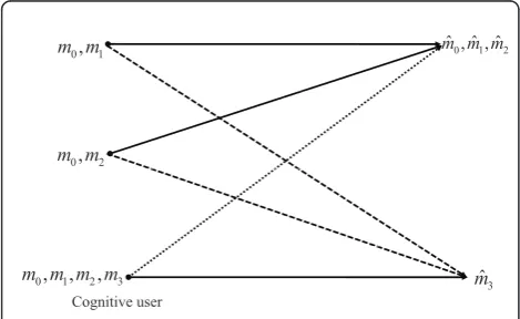
In this paper, we introduce Multiple Access-Cogni-tive Interference Channel (MA-CIFC) by providing the transmitter of the point-to-point channel with cogni-tion capabilities in the uplink with interference model. Moreover, transmitters of MAC have common infor-mation that enables cooperation among them. As shown in Figure 1, the proposed channe consists of three transmitters and two receivers: two-user MAC with common information as the primary network and a point-to-point channel with a cognitive transmitter that knows the message being sent by all of the trans-mitters in a non-causa manner. A physical example of this channel is the coexistence of cognitive users with the licensed primary users in a cellular or satellite uplink transmission, where the cognitive radios by their abilities exploit side information about the envir-onment to maintain or improve the communication of primary users while also achieving some spectrum resources for their own communication. In this sce-nario, the primary non-cognitive users can beoblivious

to the or aware of the cognitive users [1]. When the non-cognitive user is oblivious to the cognitive user’s presence, its receiver’s decoding process is independent of the interference caused by the cognitive user’s trans-mission. In fact, the primary receiver treats interfer-ence as noise. However, in the aware cognitive user’s scenario, the decoding process at the primary receiver can be adapted to improve its own rate. For example, the primary receiver can decode the cognitive user’s message and cancel the interference when the interfer-ing signal is strong enough. If the multi-antenna cap-ability is available at the primary receiver, it can also

reduce or increase the interfering signal by beam-steer-ing, which results in the occurrence of the weak or strong interference regimes [1].

To analyze the capacity region of MA-CIFC, we first derive three inner bounds on the capacity region (achiev-able rate regions). The first two bounds assume an obliv-ious primary receiver, which does not decode the cognitive user’s message but treats it as noise. Two differ-ent coding schemes are proposed based on the superposi-tion coding, the GP binning and the method of [6] in defining auxiliary Random Variables (RVs). Later, we show that these strategies are optimal for a degraded

MA-CIFC and also in the Gaussianweak interference regime. In the third achievability scheme, we consider an aware primary receiver and obtain an inner bound on the capacity region based on using superposition coding in the encoding part and allowing both receivers to decode all messages with simultaneous joint decoding in the decoding part. This strategy is capacity-achieving in the strong interference regime. Next, we provide a general outer bound on the capacity region and derive conditions under which the first achievability scheme achieves capa-city for thedegradedMA-CIFC. We continue the capa-city results by the derivation of two sets of strong interference conditions, under which the third inner bound achieves capacity. Further, we compare these two sets of conditions and identify the weaker set. We also extend the strong interference results to a network withk

primary users.

Moreover, we consider the Gaussian case and find capacity results for the Gaussian MA-CIFC in both the

weak andstronginterference regimes. We use the sec-ond derived inner bound to show that the capacity-achieving scheme in weak interference consists of Dirty Paper Coding (DPC) [22] at the cognitive transmitter and treating interference as noise at both receivers. We also provide some numerical examples.

The rest of the paper is organized as follows. Section 2 introduces MA-CIFC model and the notations. Three inner bounds and an outer bound on the capacity region are derived in Section 3 and Section 4, respectively, for the discrete memoryless MA-CIFC. Sections 5 presents the capacity results for the discrete memoryless MA-CIFC in three special cases. In Section 6, the Gaussian MA-CIFC is investigated. Finally, Section 7 concludes the paper.

2. Channel models and preliminaries

Throughout the paper, upper case letters (e.g. X) are used to denote RVs and lower case letters (e.g. x) show their realizations. The probability mass function (p.m.f) of a RV X with alphabet set _X is denoted by pX(x), where subscript Xis occasionally omitted.An_ε(X,Y) spe-cifies the set of-strongly, jointly typical sequences of

0, 1

m m m m mˆ ˆ ˆ0, ,1 2

0, 2

m m

Cognitive user

0, ,1 2, 3

m m m m mˆ₃

lengthn. The notation Xj_iindicates a sequence of RVs (Xi, Xi+1, ...,Xj), whereXjis used instead of Xj₁, for brev-ity. N(0,σ2)denotes a zero mean normal distribution with variances2.

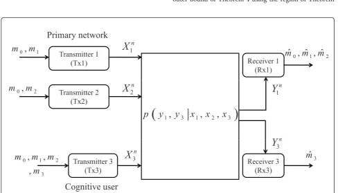
Consider the MA-CIFC in Figure 2, which is denoted by (X1×X2×X3,p(y₁n,yn₃|xn₁,xn₂,xn₃),Y1×Y3), where X1∈X1,X2∈X2 and X3∈X3 are channel inputs at Transmitter 1 (Tx1), Transmitter 2 (Tx2) and Transmit-ter 3 (Tx3), respectively;Y1∈Y1andY3∈Y3are chan-nel outputs at Receiver 1 (Rx1) and Receiver 3 (Rx3), respectively; andp(yn₁,yn₃|xn₁,xn₂,xn₃)is the channel transi-tion probability distributransi-tion. Innchannel uses, each Txj

desires to send a message pair (m0, mj) to Rx1 where j

Î{1,2}, and Tx3 desires to send a messagem3to Rx3.

Definition 1: A(2nR0_{, 2}nR1_{, 2}nR2_{, 2}nR3_,n)code for MA-CIFC consists of (i) four independent message sets Mj={1, ..., 2nRj}, wherejÎ{0, 1, 2, 3}; (ii) two encoding

functions at the primary transmitters, f1:M0×M1→X1nat Tx1 and f2:M0×M2→X2n at Tx2; (iii) an encoding function at the cognitive trans-mitter, f3:M0×M1×M2×M3→X₃n; and (iv) two decoding functions, g1:Y₁n→M0×M1×M2at Rx1 andg3:Yn

3 →M3at Rx3. We assume that the channel is memoryless. Thus, the channel transition probability distribution is given by

p(yn₁,y₃n|xn₁,xn₂,xn₃) = n

i=1

p(y1,i,y3,i|x1,i,x2,i,x3,i). (1)

The probability of error for this code is defined as

Pe=

1 2n_(R

0+R1+R2+R3)

m0,m1,m2,m3

p[{g3(Y3n)=m3}∪

{g1(Y1n)= (m0,m1,m2)}|(m0,m1,m2,m3) sent].

Definition 2: A rate quadruple (R0, R1, R2, R3) is achievable if there exists a sequence of

(2nR0_{, 2}nR1_{, 2}nR2_{, 2}nRs_{,n)codes with Pe}® _{0 as n} ® ∞_. The capacity region _C, is the closure of the set of all achievable rates.

3. Inner bounds on the capacity region of discrete memoryless MA-CIFC

Now, we derive three achievable rate regions for the general setup. Theorems 1 and 2 assume an oblivious primary receiver (Rx1), which does not decode the cog-nitive user’s message (m3) and treats it as noise. The decoding procedure at the cognitive receiver (Rx3) dif-fers in these schemes. In Theorem 1, the cognitive recei-ver (Rx3) decodes the primary messages (m0, m1, m2), and all the transmitters use superposition coding. How-ever, in Theorem 2, the cognitive receiver (Rx3) also treats the interference from the primary messages (m0,

m1, m2) as noise, while the cognitive transmitter (Tx3) uses GP binning to precode its message for interference cancelation at Rx3. We also utilize the method of [6] in defining auxiliary RVs, which helps us to achieve the outer bound in special cases. In fact, we achieve the outer bound of Theorem 4 using the region of Theorem

0

,

m

m

ˆ

ˆ

ˆ

Primary network

1

n

X

Transmitter 1

(Tx1)

Receiver 1

(Rx1)

,

m

m

0

,

,

m

m m

1

Transmitter 2

(Tx2)

,

m

m

X

Y

,

,

,

p y

y

x

x

x

n

Y

Transmitter 3

(Tx3)

,

,

m

m m

Receiver 3

m

ˆ

(Rx3)

3

n

X

n

Y

(Tx3)

,

m

Cognitive user

(Rx3)

1 for a class of degraded MA-CIFC in Section 5. The region of Theorem 2 is used in Section 6 to derive the capacity region in the weakinterference regime. In the scheme of Theorem 3, we consider an aware primary receiver (Rx1) which decodes the cognitive user’s mes-sage (m3). The cognitive receiver (Rx3) also decodes the primary messages (m0,m1, m2). Therefore, this region is obtained based on using superposition coding in the encoding part and by allowing both receivers to decode all messages with simultaneous joint decoding in the decoding part. In Section 5, we show that this strategy is capacity-achieving in the strong interference regime. Proofs are provided in“Appendix A”.

Theorem 1:The union of rate regions given by

R3≤I(X3;Y3|T,U,X1,V,X2) (2)

R1≤I(U,X1;Y1|T,V,X2) (3)

R2≤I(V,X2;Y1|T,U,X1) (4)

R1+R2≤I(U,X1,V,X2;Y1|T) (5)

R0+R1+R2≤I(T,U,X1,V,X2;Y1) (6)

R1+R3≤I(U,X1,X3;Y3|T,V,X2) (7)

R2+R3≤I(V,X2,X3;Y3|T,U,X1) (8)

R1+R2+R3≤I(U,X1,V,X2,X3;Y3|T) (9)

R0+R1+R2+R3≤I(T,U,X1,V,X2,X3;Y3) (10)

is achievable for MA-CIFC, where the union is over all p.m.fs that factor as

p(t)p(u,x1|t)p(v,x2|t)p(x3|t,u,x1,v,x2). (11)

Theorem 2:The union of rate regions given by (3)-(6) and

R3≤I(W;Y3)−I(W;T,U,X1,V,X2) (12)

is achievable for MA-CIFC, where the union is over all p.m.fs that factor as

p(t)p(u,x1|t)p(v,x2|t)p(w,x3|t,u,x1,v,x2). (13)

Theorem 3:The union of rate regions given by

R3≤I(X3;Y3|X1,X2,T) (14)

R1+R3≤min{I(X1,X3;Y1|X2,T),

I(X1,X3;Y3|X2,T)} (15)

R2+R3≤min{I(X2,X3;Y1|X1,T),

I(X2,X3;Y3|X1,T)} (16)

R0+R1+R2+R3≤min{I(X1,X2,X3;Y1),

I(X1,X2,X3;Y3)} (17)

is achievable for MA-CIFC, where the union is over all p.m.fs that factor as

p(t)p(x1|t)p(x2|t)p(x3|x1,x2,t). (18)

Remark 1: We utilize the region of Theorem 1 in Sec-tion 5 to achieve capacity results for a class of degraded MA-CIFC, and the region of Theorem 2 to derive the results for the Gaussian case in Section 6. The region of Theorem 3 is also used to characterize the capacity region under strong interference conditions in Section 5.

4. An outer bound on the capacity region of discrete memoryless MA-CIFC

Here, we derive a general outer bound on the capacity region of MA-CIFC which is used to obtain the capacity region for a class of the degraded MA-CIFC in Section 5 and also to find capacity results for the Gaussian MA-CIFC in the weak interference regime in Section 6. Let R1

odenote the union of all rate quadruples (R0,R1, R2,

R3) satisfying (3)-(6) and

R3≤I(X3;Y3,Y1|T,U,X1,V,X2), (19)

where the union is over all p.m.fs that factor as (11).

Theorem 4:The capacity region of MA-CIFC satisfies

C⊆R1 o

Proof: Consider a (2nR0_{, 2}nR1_{, 2}nR2_{, 2}nR3_{,n)code with} the average error probability ofPn_e →0. Define the fol-lowing RVs fori= 1, ...,n:

Ti= (M0,Y1i−1) (20)

Ui= (M0,M1,Y1i−1) = (M1,Ti) (21)

Vi= (M0,M2,Y1i−1) = (M2,Ti) (22)

RVs, we remark that (X1,i,Ui)®Ti®(X2,i,Vi) forms a Markov chain. Thus, these choices of auxiliary RVs satisfy the p.m.f (11) of Theorem 4. Now using Fano’s inequality [23], we derive the bounds in Theorem 4. For the first bound, we have:

nR3=H(M3)

where (a) follows since messages are independent and (b) holds due to Fano’s inequality and the fact that con-ditioning does not increase entropy. Hence,

nR3−nδ3n≤I(M3;Y3n|M0,M1,M2) defined in Definition 1, and the non-negativity of mutual information, (b) is obtained from the chain rule, (c) follows from the memoryless property of the channel and the fact that conditioning does not increase entropy, and (d) is obtained from (20)-(22).

Now, applying Fano’s inequality and the independence of the messages, we can boundR1 as:

nR1−nδ1n≤I(M1;Y1n|M0,M2)

where (a) follows from the chain rule and the encod-ing functions f1 and f2, and (b) from (20)-(22). Similarly, we can show that

Next, based on similar arguments, we bound R1 +R2 as

The last sum-rate bound can be derived as follows:

n(R0+R1+R2)−n(δ0n+δ1n+δ2n)≤I(M0,M1,M2;Y1n)

where (a) follows since conditioning does not increase entropy. Using the standard time-sharing argument for (24)-(28) completes the proof.

5. Capacity results for discrete memoryless MA-CIFC

In this section, we characterize the capacity region of MA-CIFC under specific conditions. First, we consider a class of degraded MA-CIFC and derive conditions under which the inner bound in Theorem 1 achieves the outer bound of Theorem 4. Next, we investigate the strong interference regime by deriving two sets of strong inter-ference conditions under which the region of Theorem 3 achieves capacity. We also compare these two sets of conditions and identify the weaker set. Finally, we extend the strong interference results to a network with

kprimary users.

A. Degraded MA-CIFC

Now, we characterize the capacity region for a class of MA-CIFC with adegradedprimary receiver. We define CIFC with a degraded primary receiver as a MA-CIFC whereY1and X3 are independent givenY3, X1,X2. More precisely, the following Markov chain holds:

X3|X1,X2→Y3|X1,X2→Y1|X1,X2, (29)

Assume that the following conditions are satisfied for MA-CIFC over all p.m.fs that factor as (11):

I(U,X1;Y1|T,V,X2)≤I(U,X1;Y3|T,V,X2) (30)

I(V,X2;Y1|T,U,X1)≤I(V,X2;Y3|T,U,X1) (31)

I(U,X1,V,X2;Y1|T)≤I(U,X1,V,X2;Y3|T) (32)

I(T,U,X1,V,X2;Y1)≤I(T,U,X1,V,X2;Y3) (33)

Under these conditions, the cognitive receiver (Rx3) can decode the messages of the primary users with no rate penalty. If MA-CIFC with a degraded primary recei-ver satisfies conditions (30)-(33), the region of Theorem 1 coincides with R1

oand achieves capacity, as stated in

the following theorem.

Theorem 5: The capacity region of MA-CIFC with a degraded primary receiver, defined in (29), satisfying (30)-(33) is given by the union of rate regions satisfying (2)-(6) over all joint p.m.fs (11).

Remark 2:The messages of the primary users (m0,m1,

m2) can be decoded at Rx3 under conditions (30)-(33). Therefore, Rx3-Tx3 achieves the rate in (2). Moreover, we can see that due to the degradedness condition in (29), treating interference as noise at the primary receiver (Rx1) achieves capacity. We show in Section 6 that, in the Gaus-sian case the capacity is achieved by using the region of Theorem 2 based on DPC (or GP binning), where the cog-nitive receiver (Rx3) does not decode the primary mes-sages and conditions (30)-(33) are not necessary.

Proof:Achievability: The proof follows from the region of Theorem 1. Using the condition in (30), the sum of the bounds in (2) and (3) makes the bound in (7) redun-dant. Similarly, conditions (31)-(33), along with the bound in (2), make the bounds in (8)-(10) redundant and the region reduces to (2)-(6).

Converse: To prove the converse part, we evaluateR1 o

of Theorem 4 with the degradedness condition in (29). It is noted that the p.m.f of Theorem 5 is the same as the one for R1_o. Moreover, the bounds in (3)-(6) are equal for both regions. Hence, it is only necessary to show the bound in (2). Considering (19), we obtain:

R3≤I(X3;Y3,Y1|T,U,X1,V,X2)

=I(X3;Y3|T,U,X1,V,X2) +I(X3;Y1|T,U,X1,V,X2,Y3) (a)

=I(X3;Y3|T,U,X1,V,X2)

where (a) is obtained by applying the degradedness condition in (29). This completes the proof.

B. Strong interference regime

Now, we derive two sets of strong interference condi-tions under which the region of Theorem 3 achieves

capacity. First, assume that the following set of strong interference conditions, referred to asSet1, holds for all p.m.fs that factor as (18):

I(X3;Y3|X1,X2,T)≤I(X3;Y1|X1,X2,T) (34)

I(X1,X3;Y1|X2,T)≤I(X1,X3;Y3|X2,T) (35)

I(X2,X3;Y1|X1,T)≤I(X2,X3;Y3|X1,T) (36)

I(X1,X2,X3;Y1)≤I(X1,X2,X3;Y3). (37)

In fact, under these conditions, interfering signals at the receivers are strong enough that all messages can be decoded by both receivers. Condition (34) implies that the cognitive user’s message (m3) can be decoded at Rx1, while conditions (35)-(37) guarantee the decoding of the primary messages (m0,m1, m2) along withm3at Rx3 in a MAC fashion.

Theorem 6:The capacity region of MA-CIFC satisfying (34)-(37) is given by:

Cstr 1 =

p(t)p(x1|t)p(x2|t)p(x3|x1,x2,t)

(R0,R1,R2,R3) :

R0,R1,R2,R3≥0

R3≤I(X3;Y3|X1,X2,T) (38)

R1+R3≤I(X1,X3;Y1|X2,T) (39)

R2+R3≤I(X2,X3;Y1|X1,T) (40)

R0+R1+R2+R3≤I(X1,X2,X3;Y1). (41)

Remark 3: The message of the cognitive user (m3) can be decoded at Rx1, under condition (34) and (m0, m1,

m2) can be decoded at Rx3 under conditions (35)-(37). Hence, the bound in (38) gives the capacity of a point-to-point channel with messagem3with side-information

X1,X2 at the receiver. Moreover, (38)-(41) with condi-tion (34) give the capacity region for a three-user MAC with common information where R1 and R2 are the common rates, R3 is the private rate for Tx3, and the private rates for Tx1 and Tx2 are zero.

Remark 4:If we omit Tx2, i.e., X2=∅, and Tx2 has no message to transmit, i.e., R2 = 0, the model reduces to a CIFC, andC₁strcoincides with the capacity region of the strong interference channel with unidirectional coopera-tion (or CIFC), which was characterized in [8, Theorem 5]. It is noted that in this case, the common message can be ignored, i.e.,T=∅and R0= 0.

Proof:Achievability: Considering (35)-(37), the proof follows from Theorem 3.

Converse: Consider a (2nR0_{, 2}nR1_{, 2}nR2_{, 2}nR3_{,n) code} with an average error probability of Pn_e →0. Define the following RV fori = 1, ...,n:

It is noted that due to the encoding functions f1, f2 and f3, defined in Definition 1, the independence of messages, and the above definitions forTn, RVs satisfy the p.m.f (18) of Theorem 6. First, we provide a useful lemma which we need in the proof of the converse part.

Lemma 1:If (34) holds for all distributions that factor as (18), then

I(Xn₃;Y₃n|X₁n,Xn₂,Tn,U)≤I(Xn₃;Y₁n|X₁n,Xn₂,Tn,U). (43)

Proof: The proof relies on the results in [24, Proposi-tion 1] and [25, Lemma]. By redefining X2 =X3, Y2 =

Y3,X1= (X1,X2, T) in [8, Lemma 5], the proof follows. Now, using Fano’s inequality [23], we derive the bounds in Theorem 6. Using (23) provides:

nR3−nδ3n≤I(M3;Y3n|M0,M1,M2)

where (a) is due to (42) and the encoding functionsf1,

f2 and f3, defined in Definition 1, (b) follows from two facts; conditioning does not increase entropy and

(M1,M2,M3)→(X₁n,X₂n,Xn₃)→Y₃n forms a Markov chain, (c) is obtained from the chain rule, and (d) fol-lows from the memoryless property of the channel and the fact that conditioning does not increase entropy.

Now, applying Fano’s inequality and the independence of the messages, we can boundR1 +R3as (b) follows from (42) and the fact that M3→(Xn

1,X2n,X3n)→Y3nforms a Markov chain, (c) is obtained from (43), (d) follows from the chain rule, and (e) follows from the memoryless property of the channel and the fact that conditioning does not increase entropy.

Applying similar steps, we can show that,

n(R2+R3)−n(δ2n+δ3n)≤ n

i=1

I(X2,i,X3,i;Y1,i|X1,i,T1).(46)

Finally, the sum-rate bound can be obtained as

n(R0+R1+R2+R3)−n(δ0n+δ1n+δ2n+δ3n)

where (a) follows from steps (a)-(c) in (45), (b) is due to the fact that(M1,M2)→(Xn

1,X2n,X3n)→Y1nforms a Markov chain, and (c) follows from the memoryless property of the channel and the fact that conditioning does not increase entropy. Using a standard time-shar-ing argument for (44)-(47) completes the proof.

Next, we derive the second set of strong interference conditions, called Set2, under which the region of Theo-rem 3 is the capacity region. For all p.m.fs that factor as (18),Set2includes (34) and the following conditions:

I(X1;Y1|X2,T)≤I(X1;Y3|X2,T) (48)

I(X2;Y1|X1,T)≤I(X2;Y3|X1,T) (49)

I(X1,X2;Y1)≤I(X1,X2;Y3). (50)

Theorem 7:The capacity region of MA-CIFC, satisfy-ing (34) and (48)-(50), referred to asCstr

2 , is given by the union of rate regions satisfying (14)-(17) over all p.m.fs that factor as (18).

Proof:See“Appendix B”.

Remark 6: Similar to Remark 4, by omitting

Tx2 (T=X2=∅, R0=R2= 0), the model reduces to a CIFC. Moreover, C2and Set2 reduce to the capacity region and strong interference conditions which have been derived in [13] for non-causal CIFC.

Remark 7 (Comparison of two sets of conditions):In the strong interference conditions ofSet1, the first con-dition in (34) is used in the converse part, while (35)-(37) are used to reduce the inner bound toCstr

1 . How-ever, all the conditions ofSet2are utilized to prove the converse part. Now, we compare the conditions in these two sets. We can write (35) as

I(X1;Y1|X2,T) + [I(X3;Y1|X1,X2,T)−I(X3;Y3|X1,X2,T)]

Idiff

≤I(X1;Y3|X2,T).

Considering (34), it can be seen that Idiff ≥0. Hence, condition (35) implies condition (48), but not vice versa. Similar conclusions can be drawn for other conditions of these two sets. Therefore,Set1 impliesSet2, and the conditions ofSet2are weaker compared to those ofSet1.

C. Multiple access-cognitive interference network (MA-CIFN)

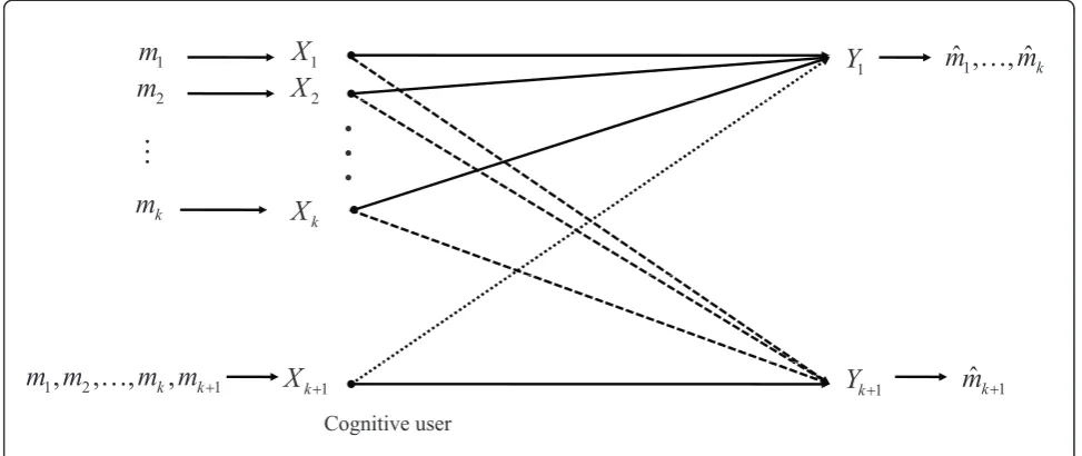
Now, we extend the result of Theorem 6 to a network with k + 1 transmitters and two receivers; a k-user MAC as a primary network and a point-to-point chan-nel with a cognitive transmitter. We call it Multiple

Access-Cognitive Interference Network (MA-CIFN). Consider MA-CIFN in Figure 3, denoted by

(X1×X2× · · · ×Xk×Xk+1,p(yn1,ynk+1|xn1,xn2,· · ·xnk,xnk+1),Y1×Yk+1), where Xj∈Xjis the channel input at Transmitter j

(Txj), for j∈ {1, ...,k+ 1};Y1∈Y1and Yk+1∈Yk+1are channel outputs at the primary and cognitive recei-vers, respectively, and p(yn₁,yn_k+1|nn₁,xn₂, ...,xn_k,xn_k+1) is the channel transition probability distribution. In n

channel uses, each Txjdesires to send a message pair

mj to the primary receiver where j Î {1, ..., k}, and Txk+ 1 desires to send a message mk+1 to the cogni-tive receiver. We ignore the common information for brevity. Definitions 1 and 2 can be simply extended to the MA-CIFN. Therefore, we state the result on the capacity region under strong interference conditions.

Corollary 1: The capacity region of the MA-CIFN, satisfying

I(Xk+1;Yk+1|X([1 :k]))≤I(Xk+1;Y1|X([1 :k])) (51)

I(Xk+1,X(S);Y1|X(Sc))≤I(Xk+1,X(S);Yk+1|X(Sc))(52)

for allS⊆[1: k] and for every p(x1)p(x2)...p(xk)p(xk+1|

x1,x2,...,xk)p(y1,yk+1|x1,x2,...,xk,xk+1), is given by

Cstr

net=

p(x1)p(x2)...p(xk)p(xk+1|x1,x2,...,xk)

{

(R1,R2,. . .,Rk,Rk+1) :R1,R2,. . .,Rk,Rk+1≥0 Rk+1≤I(Xk+1;Yk+1|X([1 :k])) (53) Rk+1+

j∈S

Rj≤I(Xk+1,X(S);Y1|X(Sc))} (54)

for allS ⊆[1:k], where X(S) is the ordered vector of

Xj, jÎS, andScdenotes the complement of the setS.

1

m

m

ˆ

, ,

!

m

ˆ

2

m

X

2

X

Y

2

#

x

2

k

m

k

X

Cognitive user

1

,

, ,

,

m m

!

m m

X

Y

m

ˆ

Proof: Following the same lines as the proof of Theo-rem 6, the proof is straightforward. Therefore, it is omitted for the sake of brevity.

Remark 8: Under condition (51), the message of the cognitive user (mk+1) can be decoded at the primary receiver (Y1). Also, the cognitive receiver (Yk+1), under condition (52), can decode mj; j Î {1,...,k} in a MAC fashion. Therefore, the bound in (53) gives the capacity of a point-to-point channel with message mk+1 with side-informationXj;jÎ {1,...,k} at the cognitive receiver. Moreover, (53) and (54) with condition (51), give the capacity region for a k + 1-user MAC with common information at the primary receiver.

6. Gaussian MA-CIFC

In this section, we consider the Gaussian MA-CIFC and characterize capacity results for the Gaussian case in the

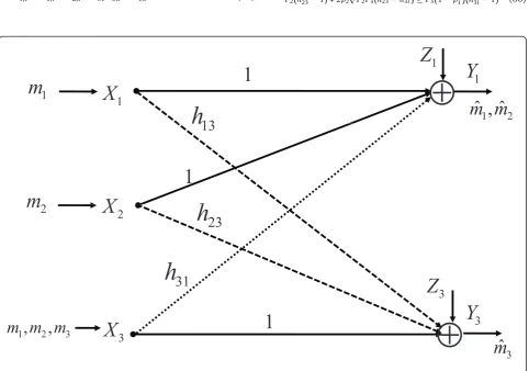
weakandstronginterference regimes. For simplicity, we assume that Tx1 and Tx2 have no common information. This means that, R0 = 0 and M0=∅. to investigate these regions. The Gaussian MA-CIFC, as depicted in Figure 4, at time i= 1,...,ncan be mathematically mod-eled as

Y1,i=X1,i+X2,i+h31X3,i+Z1,i (55)

Y3,i=h13X1,i+h23X2,i+X3,i+Z3,i (56)

where h31,h13, and h23are known channel gains.X1,i,

X2,i andX3,i are input signals with average power con-straints:

1

n n

i=1

(xj,i)2≤Pj (57)

forjÎ{1,2, 3}. Z1,iandZ3,iare independent and iden-tically distributed (i.i.d) zero mean Gaussian noise com-ponents with unit powers, i.e.,Zj,i∼N(0, 1)forjÎ {1,

3}.

A. Strong interference regime

Here, we extend the results of Theorem 6, i.e.,C₁strand

Set1, to the Gaussian case. The strong interference con-ditions of Set1, i.e., (34)-(37), for the above Gaussian model become:

h2₃₁ ≥1 (58)

P1(h213−1) + 2ρ1

P1P3(h13−h31)≥P3(1−ρ22)(h231−1) (59)

P2(h223−1) + 2ρ2

P2P3(h23−h31)≥P3(1−ρ21)(h231−1) (60)

1

X

†

Y

1

1

Z

13

h

1

1

m

1 2

ˆ ˆ

,

m m

X

13

h

h

1

m

2

X

Z

23

h

31

h

2

m

3

X

†

Y

3

3

Z

31

1

1

,

,

m m m

3

ˆ

m

P1(h2₁₃−1) +P2(h2₂₃−1) + 2ρ1

P1P3(h13−h31)

+2ρ2

P2P3(h23−h31)≥P3(h2₃₁−1)

(61)

where - 1 ≤ ru ≤ 1 is the correlation coefficient betweenXuandX3, i.e.,E(Xu,X3) =ρu

√

PuP3 foruÎ {1,

2}.

Theorem 8:For the Gaussian MA-CIFC satisfying con-ditions (58)-(61), the capacity region is given by

CG 1 =

−1≤ρ1,ρ2≤1:ρ12+ρ22≤1

{(R1,R2,R3) :R1,R2,R3≥0

R3≤θ(P3(1−ρ₁2−ρ₂2))

(62)

R1+R3≤θP1+h₃₁2P3(1−ρ₂2) + 2h31ρ1

P1P3(63)

R2+R3≤θ

P2+h2₃₁P3(1−ρ₁2) + 2h31ρ2

P2P3

(64)

R1+R2+R3≤

θP1+P2+h231P3+ 2h31

P3(ρ1

P1+ρ2

P2)

₍₆₅₎

where, to simplify notation, we define

θ(x)=. 1

2log(1 +x). (66)

Remark 9: Condition (58) implies that Tx3 causes strong interference at Rx1. This enables Rx1 to decode

m3. Moreover, (59)-(61) provide strong interference con-ditions at Rx3, under which all messages can be decoded in Rx3 in a MAC fashion.

Proof:The achievability part follows fromC₁strin Theo-rem 6 by evaluating (38)-(41) with zero mean jointly Gaussian channel inputs X1, X2 and X3. That is, X1∼N(0,P1),X2∼N(0,P2), and X3∼N(0,P3), where E(X1,X2) = 0, E(X1,X3) =ρ1

P1P3, and E(X2,X3) =ρ2

P2P3. The converse proof is based on reasoning similar to that in [26] and is provided in

“Appendix C”.

It is noted that the channel parameters, i.e.,P1,P2,P3,

h31,h13,h23, must satisfy (58)-(61) for all −1≤ρ1,ρ2≤1 :ρ12+ρ22≤1, to numerically evaluate the CG

1 using (62)-(65). Here, we choose P1=P2=P3= 6,h31 =h13=h23=√1.5 which satisfy strong interference conditions (58)-(61); hence, the regions are derived under strong interference conditions. Figure 5 shows the capacity region for the Gaussian MA-CIFC of Theorem 8, for P1 = P2 = P3 = 6, and h31 =h13=h23=√1.5, where r1 = r2 is fixed in each surface. Ther1 =r2 = 0 region corresponds to the no cooperationcase, where the channel inputs are indepen-dent. It can be seen that asr1=r2increases, the bound

0 0.5 1

1.5 2

2.5 0

0.5

1

1.5

2

2.5 0

0.5 1 1.5

R

1(bits)

R

2(bits) R 3

(bits)

ρ₁=ρ

2=0

ρ₁=ρ

2=0.4

ρ₁=ρ

2=0.6

on R3 becomes more restrictive while the sum-rate bounds become looser; because Tx3 dedicates parts of its power for cooperation. This means that, as Tx3 allo-cates more power to relaym1,m2by increasing r1=r2,

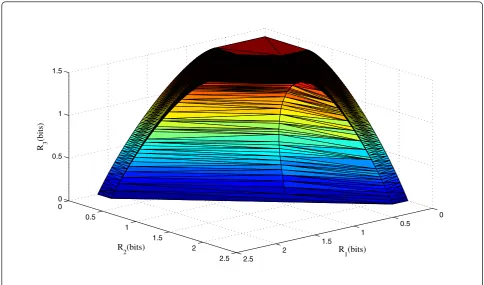
R1 and R2 improve, while R3 degrades due to the less power allocated to transmitm3. The capacity region for this channel is the union of all the regions obtained for different values ofr1and r2, satisfying ρ2

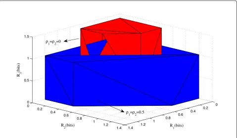
1+ρ22≤1. This union is shown in Figure 6. In order to better perceive the effect of cooperation, we letR2 = 0 in Figure 7. It is seen that by increasing r1 =r2, the bound onR1 +R3 becomes looser andR1improves, whileR3decreases due to the more power dedicated for cooperation.

B. Weak interference regime

Now, we consider the Gaussian MA-CIFC with weak interference at the primary receiver (Rx1), which means

h31 ≤1. We remark that, since there is no cooperation between receivers, the capacity region for this channel is the same as the one with the same marginal outputs p(yn

1|xn1,x2n,xn3)and p(yn3|xn1,xn2,xn3). Hence, we can state the following useful lemma.

Lemma 2: The capacity region of a Gaussian MA-CIFC, defined by (55) and (56) when h31 ≤ 1, is the same as the capacity region of a Gaussian MA-CIFC with the following channel outputs:

ˆ

Y1,i=X1,i+X2,i+h31Y3,i+Z1,i (67)

Y3,i=h13X1,i+h23X2,i+Y3,i (68)

where Y’3,i = X3,i + Z3,i and Z1,i∼N(0, 1−h231). Therefore, the degradedness condition in (29) holds for the Gaussian MA-CIFC whenh31≤1.

Proof:The proof follows from [6, Lemma 3.5].

Next, we use the inner bound of Theorem 2 and the outer bound of Theorem 4 to derive the capacity region, which shows that the capacity-achieving scheme in this case consists of DPC at the cognitive transmitter and treating interference as noise at both receivers.

Theorem 9: For the Gaussian MA-CIFC, defined by (55) and (56), whenh31≤1, the capacity region is given by

CG 2 =

−1≤ρ1,ρ2≤1:ρ12+ρ22≤1

{(R1,R2,R3) :R1,R2,R3≥0

R3≤θ(P3(1−ρ₁2−ρ₂2))

(69)

R1≤θ

(√P1+h31ρ1 √

P3)2

h2₃₁P3(1−ρ₁2−ρ2₂) + 1

(70)

0 0.5 1

1.5 2

2.5 0

0.5

1

1.5

2

2.5 0

0.5 1 1.5

R

1(bits)

R

2(bits) R 3

(bits)

R2≤θ

(√P2+h31ρ2 √

P3)2

h2₃₁P3(1−ρ₁2−ρ₂2) + 1

(71)

R1+R2≤

θ

√

P1+h31ρ1 √

P3

2

+√P2+h31ρ2 √

P3

2

h2

31P3(1−ρ21−ρ22) + 1

(72)

whereθ(·) is defined in (66).

Remark 10: By evaluating (2) with jointly Gaussian channel inputs, one can easily achieve (69). However, this results in the Gaussian counterparts of the bounds in (7)-(10). Therefore, some conditions are necessary to make these bounds redundant, similar to the ones in (30)-(33). However, we show that (12) is also evaluated to (69), if we apply DPC with appropriate parameters. Hence, conditions (30)-(33) are unnecessary in the Gaussian case. This means that DPC completely miti-gates the effects of interference for the Tx3-Rx3 pair and leaves the link between them interference-free for fixed values ofr1, r2. Consequently,CG

2 is independent ofh13andh23.

Remark 11: If we omit Tx2, the model reduces to a CIFC and by settingP2=ρ2=R2= 0,C2Gcoincides with the capacity region of the Gaussian CIFC with weak interference, which was characterized in [6, Lemma 3.6].

Proof: The rate region in Theorem 2 can be extended to the discrete-time Gaussian memoryless case with continuous alphabets by standard arguments [23]. Hence, it is sufficient to evaluate (3)-(6) and (12) with an appropriate choice of input distribution to reach (69)-(72). LetR0= 0,M0=∅, andT=∅, since Tx1 and Tx2 have no common information. Also, letUand Vbe deterministic constants. We choose zero mean jointly Gaussian channel inputs X1, X2 and X3. In fact, Xj∼N(0,Pj) for j Î {1,2,3}, where E(X1,X2) = 0, E(X1,X3) =ρ1

P1P3, and E(X2,X3) =ρ2

P2P3. Noting the p.m.f (13), consider the following choice of input distribution for certain{−1≤ρ1,ρ2≤1 :ρ12+ρ22≤1}:

X1∼N(0,P1),X2∼N(0,P2)

W=X3+α1X1+α2X2,X3∼N(0, (1−ρ12−ρ22)P3)

X3=X3+ρ1

P3 P1X1+ρ2

P3 P2X2

(73)

Therefore, (3)-(6) are easily evaluated to (70)-(72). In

“Appendix D”, we derive (69) by evaluating (12) with appropriate parameters. The converse proof follows by applying the bounds in the proof of Theorem 4 to the Gaussian case and utilizing Entropy Power Inequality (EPI) [23,27]. A detailed converse proof is provided in

“Appendix D”.

0 0.5 1 1.5 2 2.5

0 0.5 1 1.5

R

1(bits)

R 3

(bits)

ρ₁2

=ρ

2 2

=0.5

ρ₁=ρ

2=0

ρ₁=ρ

2 increases

Remark 12: According to Theorems 8 and 9, jointly Gaussian channel inputsX1,X2 andX3 are optimal for the Gaussian MA-CIFC under the strong and weak interference conditions, determined in the above theorems.

Figure 8 shows the capacity region for the Gaussian MA-CIFC of Theorem 9, for P1 = P2 = P3 = 6, and h31=√0.55, wherer1 =r2 is fixed in each surface. It is noted that the capacity region is independent ofh13and

h23. Ther1=r2= 0 region corresponds to theno

coop-eration case, where channel inputs are independent. We see that when Tx3 dedicates parts of its power for coop-eration, i.e.,r1 =r2 = 0.5, the rates of the primary users (R1, R2) increase, whileR3decreases. The capacity region for this channel is the union of all the regions obtained for different values of r1 andr2 satisfying,_ρ2

1+ρ22≤1, which is shown in Figure 9. Similar to Figure 7, we investigate the capacity region forR2= 0 in Figure 10 in the weak interference regime. It is seen that, when Tx3 dedicates more power for cooperation by increasingr1 =r2,R1improves andR3decreases.

7. Conclusion

We investigated a cognitive communication network where a MAC with common information and a point-to-point channel share a same medium and interfere with each other. For this purpose, we introduced

Multiple Access-Cognitive Interference Channel (MA-CIFC) by merging a two-user MAC as a primary net-work and a cognitive transmitter-receiver pair in which the cognitive transmitter knows the message being sent by all of the transmitters in a non-causal manner. We analyzed the capacity region of MA-CIFC by deriving the inner and outer bounds on the capacity region of this channel. These bounds were proved to be tight in some special cases. Therefore, we determined the opti-mal strategy in these cases. Specifically, in the discrete memoryless case, we established the capacity regions for a class of degradedMA-CIFC and also under two sets of strong interference conditions. We also derive strong interference conditions for a network with kprimary users. Further, we characterized the capacity region of the Gaussian MA-CIFC in theweakandstrong interfer-ence regimes. We showed that DPC at the cognitive transmitter and treating interference as noise at the receivers, i.e., an oblivious primary receiver, are optimal in the weak interference. However, the receivers have to decode all messages when the interference is strong enough, which requires an aware primary receiver.

Appendix A Proofs of Theorems 1, 2 and 3

Outline of the proof for Theorem 1:We propose the fol-lowing random coding scheme, which contains superpo-sition coding and the technique of [6] in defining

0 0.2 0.4 0.6 0.8 1 1.2 1.4 0

0.2 0.4

0.6 0.8

1 1.2

1.4 0

0.5 1 1.5

R

1(bits)

R

2(bits) R 3

(bits)

ρ₁=ρ

2=0

ρ₁=ρ

2=0.5

0 0.5 1

1.5 2

2.5 0

0.5 1

1.5 2

2.5 0

0.5 1 1.5

R

1(bits)

R₂(bits)

R 3

(bits)

Figure 9The capacity region for the weak Gaussian MA-CIFC.

0 0.2 0.4 0.6 0.8 1 1.2 1.4 1.6 1.8 2

0 0.5 1 1.5

R₁(bits)

R3

(bits)

ρ₁2

=ρ

2 2

=0.5

ρ₁=ρ

2=0

ρ₁=ρ

2 increases

auxiliary RVs, i.e.,Uand V. The cognitive receiver (Rx3) decodes the interfering signals caused by the primary messages (m1, m2), while the primary receiver (Rx1) does not decode the interference from the cognitive user’s message (m3) and treats it as noise.

Codebook Generation: Fix a joint p.m.f as (11). Gen-erate₂nR0i.i.dtnsequences, according to the probability

n generate 2nR3 i.i.d xn₃ sequences, according to

n

Rx1: After receivingyn₁, Rx1 looks for a unique triple

(m0ˆ ,m1ˆ ,m2ˆ )and somem2_ˆ such that

(yn₁,tn(m0 ),un(m0 ,m1),xn1(m0 ,m1),vn(m0,m2 ), xn₂(m0,m2))∈An_∈(Y1,T,U,X1,V,X2).

For large enoughn with arbitrarily high probability,

(m0ˆ ,m1ˆ ,m2ˆ ) = (m0,m1,m2)if (3)-(6) hold.

Rx3: After receivingyn₃, Rx3 finds a unique index_m3ˆˆ and some triple(m0ˆˆ ,m1ˆˆ ,m2ˆˆ )such that

With arbitrary high probability,_m3ˆˆ _=m3if n is large enough and (2), (7)-(10) hold. This completes the proof.

Outline of the proof for Theorem 2:Our proposed ran-dom coding scheme, in the encoding part, contains the methods of Theorem 1 and GP binning at the cognitive transmitter (Tx3) which is used at Tx3 to cancel the interference caused bym0,m1, m2at Rx3. In the decod-ing part, both receivers decode only their intended mes-sages, treating the interference as noise. Therefore, unlike the decoding part of Theorem 1, Rx3 decodes

only its own message (m3), while treating the other sig-nals as noise.

Codebook Generation: Fix a joint p.m.f as (13). Gen-eratetn_(m

0),un(m0,m1),xn1(m0,m1),vn(m0,m2),xn2(m0,m2)

codewords based on the same lines as in the codebook generationpart of Theorem 1. Then, generate₂n(R3+L)i.i.

If there is more than one such index, Tx3 picks the smallest. If there is no such codeword, it declares an error. Using covering lemma [27], it can be shown that there exists such an indexl with high enough probabil-ity ifnis sufficiently large and

L≥I(W;T,U,X1,V,X2). (74)

Then, Tx3 sends xn₃ generated according to

n

i=1

p(x3,i|ti,ui,x1,i,vi,x2,i).

Decoding: The decoding procedure at Rx1 is similar to Theorem 1 and the error in this receiver can be bounded if (3)-(6) hold.

Rx3: After receivingy₃n, Rx3 finds a unique index_m3ˆˆ for some indexˆˆ_lsuch that

yn₃,wnm3 ,l∈An_∈(Y3,W).

For large enough n, the probability of error can be made sufficiently small if

R3+L≤I(W;Y3). (75)

Combining (74) and (75) results in (12). This com-pletes the proof.

Outline of the proof for Theorem 3: We propose the following random coding scheme, which contains super-position coding in the encoding part and simultaneous joint decoding in the decoding part. All messages are common to both receivers, i.e., both receivers decode (m0,m1,m2,m3).

Codebook Generation: Fix a joint p.m.f as (18). Gen-erate2nR0i.i.dtnsequences, according to the probability

n

i=1

Î {1,2} and eachtn(m0), generate2nRji.i.dxnj sequences,

each with probability

n

i=1

p(xj,i|ti). Index them as

xn_j(m0,mj) where mj∈[1, 2nRj]. For each (tn_(m

0),xn1(m0,m1),xn2(m0,m2)), generate 2nR3 i.i.d xn₃ sequences, each with probability

n

i=1

p(x3,i|ti,x1,i,x2,i).

Index them asxn₃(m0,m1,m2,m3)wherem3∈[1, 2nR3_].

Encoding: In order to transmit message (m0,m1, m2,

m3), Txjsends x

n

j(m0,mj)for j Î {1,2} and Tx3 sends xn₃(m0,m1,m2,m3).

Decoding:

Rx1: After receivingyn₁, Rx1 looks for a unique triple

(mˆ0,mˆ1,mˆ2)and somem3ˆ such that

(yn1,tn(m0),x1n(m0,m1), xn2(m0,m2),xn3(m0,m1,m2,m3)) ∈An_∈(Y1,T,X1,X2,X3).

For large enoughn, with arbitrarily high probability

(m0ˆ ,m1ˆ ,m2ˆ ) = (m0,m1,m2)if

R1+R3≤I(X1,X3;Y1|X2,T) (76)

R2+R3≤I(X2,X3;Y1|X1,T) (77)

R0+R1+R2+R3≤I(X1,X2,X3;Y1). (78)

Rx3: Similarly, after receivingyn₃, Rx3 finds a unique index_m3ˆˆ and some triple(m0ˆˆ ,m1ˆˆ ,m2ˆˆ )such that

(yn3,tn(mˆˆ0),x1n(mˆˆ0,mˆˆ1),xn2(mˆˆ0,mˆˆ2),xn3(mˆˆ0,mˆˆ1,mˆˆ2,mˆˆ3)) ∈An_ε(Y3,T,X1,X2,X3).

With the arbitrary high probability _m3ˆˆ _=m3, if n is large enough and

R3≤I(X3;Y3|X1,X2,T) (79)

R1+R3≤I(X1,X3;Y3|X2,T) (80)

R2+R3≤I(X2,X3;Y3|X1,T) (81)

R0+R1+R2+R3≤I(X1,X2;Y3|X1). (82)

This completes the proof.

Appendix B Proof of Theorem 7

Since achievability directly follows from Theorem 3, we proceed to the converse part. We assume a code with the properties indicated in the converse proof of Theo-rem 6 and defineTnas (42). Four bounds inCstr₂ are the same as the bounds inC₁str, which are shown in the con-verse proof of Theorem 6. Therefore, it is necessary to

prove the three bounds. Moreover, similar to Lemma 1, we have:

Lemma 3: If (48)-(50) hold for all distributions that factor as (18), then

I(Xn₁;Y₁n|Xn₂,Tn)≤I(Xn₁;Y₃n|Xn₂,Tn) (83)

I(Xn₂;Y₁n|Xn₁,Tn)≤I(Xn₂;Y₃n|Xn₁,Tn) (84)

I(Xn₁;Xn₂;Y₁n)≤I(Xn₁;Y₂n|X₃n). (85)

We next prove the remaining three bounds of Theo-rem 7. Applying Fano’s inequality, similar to (45), we have:

n(R1+R3)−n(δ1n+δ3n)

≤I(M1,Xn1;Y1n|M0,M2,Xn2) +I(Xn3;Yn3|M0,M1,M2,Xn1,Xn2) (a)

=I(Xn

1;Y1n|Tn,M2,Xn2) +I(X3n;Y3n|Tn,M1,M2,Xn1,X2n) (b)

≤I(X₁n;Y₃n|Tn,M2,X2n) +I(Xn3;Y3n|Tn,M1,M2,Xn1,X2n) (c)

≤I(M1,Xn1,X3n;Y3n|Tn,M2,Xn2) (d)

≤ n

i=1

I(X1,i,X3,i;Y3,i|X2,i,Ti)

(86)

where (a) follows from (42) and the deterministic rela-tion betweenX₁nandM1, (b) is obtained from (83), (c) is due to the fact that mutual information is non-negative, and (d) follows from the facts that conditioning does not increase entropy and the channel is memoryless.

Using a similar approach and condition (84), it can be shown that

n(R2+R3)−n(δ2n+δ3n)≤ n

i=1

I(X2,i,X3,iY3,i|X1,i,Ti). (87)

Finally, using (47) we obtain the last sum-rate bound as:

n(R0+R1+R2+R3)−n(δ0n+δ1n+δ2n+δ3n)

≤I(M0,M1,M2,Xn₁,Xn₂;Y₁n)

+I(X₃n;Y₃n|M0,M1,M2,X₁n,X₂n)

(a)

≤I(Xn₁,X₂n;Y₁n) +I(Xn₃;Y₃n|Xn₁,X₂n)

(b)

≤I(X₁n,X₂n;Y₃n) +I(X₃n;Y₃n|X₁n,X₂n)

=I(Xn₁,Xn₂,Xn₃;Y₃n)≤ n

i=1

I(X1,i,X2,iX3,i;Y3,i)

(88)

where (a) is obtained from the deterministic relation between Xn

Appendix C Proof of the converse part for Theorem 8

For any rate triple(R1,R2R3)∈C, Rx1 is able to decode

m1and m2reliably. Then, Rx1 is able to construct

˜

If condition (58) holds, thenY3˜ is a less noisy version of

Y3. Since Rx3 has to decodem3, Rx1 can decodem3via ˜

Y3with no rate penalty. Therefore, (R1,R2,R3) is con-tained in the capacity region of a three-user MAC with common information [19] at Rx1, whereR1andR2are the common rates between Tx1-Tx3 and Tx2-Tx3, respectively;R3is the private rate for Tx3; and the private rates for Tx1 and Tx2 are zero. From the maximum entropy theorem [23], this region is largest for Gaussian inputs and is evaluated to (63)-(65). The bound in (62) follows by applying the standard methods as in (44).

Appendix D Detailed proof for Theorem 9

First, we derive (69) by evaluating (12) with appropriate parameters. Consider the mapping in (73). We choose

α1=β

Z3 uncorrelated and hence independent since they are jointly Gaussian. Using (12) and (73), we obtain

I(W;Y3)−I(W;T,U,X1,V,X2) =h(W|X1,X2)−h(W|Y3)

where (a) follows from (89), (90), and

Y13+ρ1

X1 andX2 are jointly independent. By applying (93) to (92), we can evaluate (12) as:

h(X3)−h(W|Y3) =h(X3)−h(X3|X3+Z3)

=I(X3;X3+Z3) =θ(P3(1−ρ21−ρ 2 2)) This completes the achievability proof.

Converse: Utilizing the power constraint (57), we derive the bounds of R1

ofor the Gaussian MA-CIFC

when h31< 1. It can be easily shown that we can set T=∅, sinceR0 = 0 andM0=∅. Applying the degraded-ness condition (29) to (19), which holds due to Lemma 2, we obtain:

Using the fact that conditioning does not increase the entropy and (57) withj= 3 yields:

h(Y3|U,X1,V,X2)≥h(Y3|U,X1,V,X2,X3) =

Combining (94) and (95) results in

R3≤I(X3;Y3|U,X1,V,X2) = 1

2log(λP3+ 1) (96)

for some 0≤l ≤1. Now, considering that the Gaus-sian distribution maximizes the entropy of a RV for a given value of the second moment, we have:

h(Y3|U,X1,V,X2)≤h(X3+Z3|X1,X2)

P2P3 . Considering (95) and (97), we obtain:

λ≤1−ρ₁2−ρ₂2

λ= 1−ρ₁2−ρ₂2. (98)

Consequently, (69) follows from (96) and (98). Now, consider the bound in (3):

R1≤h(Y1|V,X2)−h(Y1|U,X1,V,X2). (99)

We can compute the first term as

h(Y1|V, X2)

which incorporates the fact that Gaussian distribution maximizes the entropy of a RV for a given value of the second moment.

To compute the second term in (99), the Entropy Power Inequality (EPI) [23,27] is used to obtain:

22h(Y1|U,X1,V,X2) (_{= 2}a) 2h(h31Y3+Z1|U,X1,V,X2)

where (a) follows from (67), (b) is obtained from EPI, and (c) follows from (95) and (98). Therefore, (3) is evaluated to (70) by combining (99)-(101).

Utilizing (101), one can easily evaluate (4) and (5) to (71) and (72), respectively. This completes the converse proof for Theorem 9.

Acknowledgements

This work was partially supported by Iran National Science Foundation (INSF) under contract No. 88114.46-2010 and by Iran Telecom Research Center (ITRC) under contract No. T500/17865. The material in this paper has been presented in part in the Canadian Workshop on Information Theory (CWIT), Kelowna, British Columbia, Canada, May 17-20, 2011.

Competing interests

The authors declare that they have no competing interests.

Received: 18 May 2011 Accepted: 1 November 2011 Published: 1 November 2011

References

1. A Goldsmith, SA Jafar, I Maric, S Srinivasa, Breaking spectrum gridlock with cognitive radios: an information theoretic perspective. Proc ieee, invited.

97(5), 894–914 (2009)

2. N Devroye, P Mitran, V Tarokh, Achievable rates in cognitive radio channels. ieee Trans Inf Theory.52, 1813_–1827 (2006)

3. S Gel’fand, M Pinsker, Coding for channels with random parameters. Probl Control Info Theory.9(1), 19_–31 (1980)

4. TS Han, K Kobayashi, A new achievable rate region for the interference channel. ieee Trans Inf Theory.27, 49_–60 (1981). doi:10.1109/ TIT.1981.1056307

5. A Jovicic, P Viswanath, Cognitive radio: an information-theoretic perspective. ieee Trans Inf Theory.55, 3945–3958 (2009)

6. W Wu, S Vishwanath, A Arapostathis, Capacity of a class of cognitive radio channels: interference channels with degraded message sets. ieee Trans Inf Theory.53(11), 4391–4399 (2007)

7. N Devroye, M Vu, V Tarokh, Achievable rates and scaling Laws in cognitive radio channels. EURASIP J Wirel Commun Netw Special issue on cognitive radio and dynamic spectrum sharing systems.2008(896246) (2008) 8. I Maric, RD Yates, G Kramer, Capacity of interference channels with partial

transmitter cooperation. IEEE Trans Inf Theory.53, 3536–3548 (2007) 9. I Maric, A Goldsmith, G Kramer, S Shamai (Shitz), On the capacity of interference channels with one cooperating transmitter. Eur Trans Telecommun.19, 405_–420 (2008). doi:10.1002/ett.1298

10. S Rini, D Tuninetti, N Devroye, State of the cognitive interference channel: a new unified inner bound, and capacity to within 1.87 bits, inProceedings of the 2010 International Zurich Seminar on Communicationshttp://arxiv.org/ abs/0910.3028v1

11. S Rini, D Tuninetti, B Devroye, New inner and outer bounds for the discrete memoryless cognitive interference channel and some capacity results. http://arxiv.org/abs/1003.4328v1 (2010)

12. M Mirmohseni, B Akhbari, MR Aref, On the capacity of interference channel with causal and non-causal generalized feedback at the cognitive transmitter. IEEE Trans Inf Theoryhttp://ee.sharif.ir/~mirmohseni/IT-prep.pdf. submitted to, April 2010, Revised, Oct. 2011.

13. M Mirmohseni, B Akhbari, MR Aref, Capacity regions for some classes of causal cognitive interference channels with delay, inProceedings of the IEEE Information Theory Workshop (ITW), (Dublin, 2010)

14. J Jiang, Y Xin, On the achievable rate regions for interference channels with degraded message sets. IEEE Trans Inf Theory.54, 4707_–4712 (2008) 15. KG Nagananda, CR Murthy, Three-user cognitive channels with cumulative

message sharing: an achievable rate region, inProceedings of the IEEE Information Theory Workshop (ITW), (Greece, 2009), pp. 291–295 16. KG Nagananda, CR Murthy, Information theoretic results for three-user

cognitive channels, inProceedings of the IEEE Globecom(2009)

17. R Ahlswede, Multiway communication channels. In: Proceedings of the IEEE International Symposium Information Theory (ISIT), (Tsahkadsor, Armenian S. S.R, 1971), pp. 23–52

18. HHJ Liao, Multiple access channels, (University of Hawaii, Honolulu, 1972) Ph.D. Thesis

19. D Slepian, JK Wolf, A coding theorem for multiple access channels with correlated sources. Bell Syst Tech J.52, 1037–1076 (1973)

20. A Chaaban, A Sezgin, On the capacity of the 2-user Gaussian MAC interfering with a P2P link. http://arxiv.org/abs/1010.6255v1 (2010) 21. F Zhu, X Shang, B Chen, HV Poor, On the capacity of

multiple-access-Z-interference channels. http://arxiv.org/abs/1011.1225v1 (2010) 22. MHM Costa, Writing on dirty paper. IEEE Trans Inf Theory.29, 439–441

(1983). doi:10.1109/TIT.1983.1056659

23. TM Cover, JA Thomas, Elements of Information Theory, 2nd edn. (Wiley Series in Telecommunications, 2006)

24. J Koörner, K Marton, Comparison of two noisy channels, inTopics in information theory, ed. by I Csiszar, P Elias (North-Holland, Amsterdam, 1977). Colloquia Mathematica Societatis Janos Bolyai

25. MHM Costa, A El Gamal, The capacity region of the discrete mem-oryless interference channel with strong interference. IEEE Trans Inf Theory.33(5), 710–711 (1987). doi:10.1109/TIT.1987.1057340

26. H Sato, The capacity of the Gaussian interference channel under strong interference. IEEE Trans Inf Theory.27(6), 786–788 (1981). doi:10.1109/ TIT.1981.1056416

27. A El Gamal, YH Kim, Lecture notes on network information theory. http:// arxiv.org/abs/1001.3404 (2010). [Online]. Available

doi:10.1186/1687-1499-2011-152