R E S E A R C H
Open Access
A space-time spectral method for the time
fractional diffusion optimal control problems
Xingyang Ye
1and Chuanju Xu
2**Correspondence: [email protected] 2School of Mathematical Sciences, Xiamen University, Xiamen, 361005, China
Full list of author information is available at the end of the article
Abstract
In this paper, we study the Galerkin spectral approximation to an unconstrained convex distributed optimal control problem governed by the time fractional diffusion equation. We construct a suitable weak formulation, study its well-posedness, and design a Galerkin spectral method for its numerical solution. The contribution of the paper is twofold:a priorierror estimate for the spectral approximation is derived; a conjugate gradient optimization algorithm is designed to efficiently solve the discrete optimization problem. In addition, some numerical experiments are carried out to confirm the efficiency of the proposed method. The obtained numerical results show that the convergence is exponential for smooth exact solutions.
Keywords: fractional optimal control problem; time fractional diffusion equation; spectral method;a priorierror
1 Introduction
Optimal control problems (OCPs) can be found in many scientific and engineering ap-plications, and it has become a very active and successful research area in recent years. Considerable work has been done in the area of OCPs governed by integral order differ-ential equations, the literature on this field is huge, and it is impossible to give even a very brief review here. Recently, fractional differential equations (FDEs) have gained consid-erable importance due to their application in various sciences, such as control theory [, ], viscoelastic materials [, ], anomalous diffusion [–], advection and dispersion of solutes in porous or fractured media [],etc.[–]. Therefore, the optimal control prob-lem for the fractional-order system initiated a new research direction and has received increasing attention.
A general formulation and a solution scheme for the fractional optimal control prob-lem (FOCP) were first proposed in [], where the fractional variational principle and the Lagrange multiplier technique were used. Following this idea, Frederico and Torres [, ] formulated a Noether-type theorem in the general context and studied fractional con-servation laws. Mophou [] applied the classical control theory to a fractional diffusion equation, involving a Riemann-Liouville fractional time derivative. Dorvilleet al.[] later extended the results of [] to a boundary fractional optimal control. Also we refer the in-terested reader in FOCP to [–] for some recent work on the subject.
Recently, considerable efforts have been made in developing spectral methods for solv-ing FDEs. For instance, a Legendre spectral approximation was proposed in [–] to
solve the fractional diffusion equations. Bhrawyet al.[] applied the shifted Legendre spectral collocation method to obtain the numerical solution of the space-time fractional Burger’s equation. A spectral collocation scheme based upon the generalized Laguerre polynomials was investigated in [] to obtain a numerical solution of the fractional pan-tograph equation with variable coefficients on a semi-infinite domain. With the help of operational matrices of fractional derivatives for orthogonal polynomials, the Jacobi tau spectral method is also utilized in [] to solve multi-term space-time fractional par-tial differenpar-tial equations. On the other hand, there exist also limited but very promis-ing efforts in developpromis-ing spectral methods for solvpromis-ing FOCPs. In [], a numerical direct method based on the Legendre orthonormal basis and operational matrix of Riemann-Liouville fractional integration were introduced to solve a general class of FOCP, and the convergence of the proposed method was also extensively discussed. Ye and Xu [] proposed a Galerkin spectral method to solve the linear-quadratic FOCP associ-ated to the time fractional diffusion equation with control constraints, and detailed er-ror analysis was carried out. Doha et al. [] derived an efficient numerical scheme based on the shifted orthonormal Jacobi polynomials to solve a general form of the FOCPs.
The main aim of this work is to derivea priorierror estimates for spectral approxima-tion to an unconstrained FOCP with general convex cost funcapproxima-tional, and propose an effi-cient algorithm to solve the discrete control problem. As compared to the linear-quadratic FOCP considered by Ye and Xu [], the presence of the general cost functional here leads to many additional difficulties, one of which is that the derivation of the optimality con-dition.
The rest of the paper is organized as follows. In the next section we formulate the op-timal control problem under consideration and derive the opop-timality conditions. In Sec-tion , the space-time spectral discretizaSec-tion is presented. Thereafter, the main result on the error analysis for the considered optimal control problem is given in Section . In this section, error estimates for the error in the control, state, and adjoint variables are analyzed. In Section , we describe the overall algorithm and present some numerical examples to illustrate our results. Some concluding remarks are given at the end of this article.
2 Fractional optimal control problem and optimization
Let= (–, ),I= (,T), and=I×. We consider the following optimal control prob-lem for the state variableuand the control variableq:
min
q
g(u) +h(q), (.)
wheregandhare given convex functionals,uis governed by the time fractional diffusion equation as follows:
∂tαu(x,t) –∂xu(x,t) =f(x,t) +q(x,t), ∀(x,t)∈,
u(–,t) =u(,t) = , ∀t∈I, (.)
with∂tαdenoting the left-sided Caputo fractional derivative of orderα∈(, ), following
In order to define well the FOCP, we first introduce some notations that will be used to construct the weak problem of the time fractional diffusion equation (.). We use the symbolOto denote a domain which may stand for,Ior. LetL(O) be the space of
measurable functions whose square is Lebesgue integrable inO. The inner product and norm ofL(O) are defined by
Particularly, we will need to recall the definitions of some fractional Sobolev spaces in-troduced in []. For a bounded domainI, the space
lHs(I) :=v;v
lHs(I)<∞
is endowed with the norm
vlHs(I):=
is endowed with the norm
vrHs(I):=v
∂tsvandRt∂Tsv, respectively, denote the left and right Riemann-Liouville fractional
derivative, whose definitions will be given later. It has been showed in [] that the spaces
We also need some definitions regarding fractional derivatives allowing us to formulate the FOCP. The right Caputo fractional derivative [] is given by
t∂Tαu(t) = –
The left Riemann-Liouville fractional derivative is defined as
R
and the right Riemann-Liouville fractional derivative is given by
R
The definitions of the Riemann-Liouville and the Caputo fractional derivative are linked by the following relationship:
We employ the space introduced in []
Bs() =HsI,L()∩LI,H()
In this setting, the weak formulation of the state equation (.) reads []: givenq,f ∈ L(), findu∈Bα(), such that
It has been proved [] that the problem (.) is well-posed. We now define the cost functional as follows:
We further assume thath(q)→+∞asq,→+∞, and the functionalg(·) is bounded
below, then the optimal control problem (.) admits a unique solution (q∗,u(q∗))∈ L()×Bα().
The well-posedness of the state problem ensures the existence of a control-to-state map-ping q→u=u(q) defined through (.). By means of this mapping we introduce the reduced cost functionalJ(q) :=J(q,u(q)),q∈L(). Then the optimal control problem
(.) is equivalent to: findq∗∈L(), such that
Jq∗= min
q∈L()J(q). (.) The first order necessary optimality condition for (.) takes the form
Jq∗(δq) = , ∀δq∈L(), (.)
whereJ(q∗)(δq) is usually called the gradient ofJ(q), which is defined through the Gâteaux differential ofJ(q) atq∗along the directionδq.
Lemma . We have
J(q)(δq) =h(q) +z(q),δq, ∀δq∈L(), (.)
where z(q) =z is the solution of the following adjoint state equation:
t∂Tαz(x,t) –∂xz(x,t) =g(u), ∀(x,t)∈,
z(–,t) =z(,t) = , ∀t∈I, (.)
z(x,T) = , ∀x∈.
Proof We first obtain by using the chain rule
J(q)(δq) =gu(q)(δq) +h(q)(δq)
=
gu(q)u(q)(δq) dxdt+
h(q)δqdxdt. (.)
We now computeu(q)(δq). For simplicity, letδudenote the derivative ofu=u(q) in the directionδq, that is,
δu(x,t) :=u(q)(δq) =lim
ε→
u(q+εδq) –u(q)
ε .
Then it is readily seen thatδuis the solution of the following problem:
⎧ ⎪ ⎪ ⎨ ⎪ ⎪ ⎩
∂tαδu–∂xδu=δq, ∀(x,t)∈, δu(–,t) =δu(,t) = , ∀t∈I,
δu(x, ) = , ∀x∈.
To prove (.), we multiply each side of the first equation in (.) byδu, then integrate the resulted equation on the domainto find
On one side, taking into account the boundary conditions in (.) and (.), we have
On the other side, by means of (.), (.), the terminal condition in (.), the initial condition in (.), and the fractional integration by parts demonstrated in [], we have
Finally, combining (.), (.), (.), and (.), we obtain
Following the same idea as for the problem (.), it can be proved that (.) admits a unique solutionz∈Bα() for any givenu∈Bα().
In what follows we will need the mappingq→u(q)→z(q), where for any givenq,u(q) is defined by (.), and onceu(q) is knownz(q) is defined by (.).
3 Space-time spectral discretization
In this section we investigate a space-time spectral approximation to the optimization problem (.).
We first define the polynomial space
PM() :=PM()∩H(), SL:=PM()⊗PN(I),
wherePMdenotes the space of all polynomials of degree less than or equal toM,Lstands
We then define the discrete cost functional, which is an approximation to the reduced cost functionalJ, as follows:
JL(qL) :=g(uL) +h(qL), ∀qL∈PM()⊗PN(I), (.)
We propose the following space-time spectral approximation to the optimization problem (.): findq∗L∈PM()⊗PN(I) such that
It can be proved that the discrete optimization problem (.) admits a unique solution q∗L∈PM()⊗PN(I), which fulfills the first order optimality condition:
4 A priori error estimation
We now carry out an error analysis for the spectral approximation (.). To simplify the notations, we letcbe a generic positive constant independent of any functions and of any discretization parameters. We use the expressionABto mean thatA≤cB.
We now introduce the auxiliary problem:
AuL(q),vL then it can be verified by a direct calculation that
JL(q)(δq) =h(q) +zL(q),δq
, δq∈L
(). (.)
Lemma . For any q∈L(),let u(q)be the solution of(.),u
We are now in a position to analyze the approximation error of the proposed space-time spectral method. The proof of the main result will be accomplished with a series of lemmas which we present below.
Lemma . If g(·)is convex and h(·)is uniformly convex,that is,there exists a constant c
Moreover, it follows from (.) and (.) that
Lemma . Let q∗ be the solution of the continuous optimization problem(.),q∗Lbe the solution of the discrete optimization problem (.). Assume that h(·) and g(·) are Lipschitz continuous with Lipschitz constants L and L,respectively.Moreover,suppose
q∗∈L(I;Hμ())∩Hν(I;L()),ν> ,μ≥,then we have
q∗–q∗L,N–νq∗,ν+M–μq∗μ,+zL
q∗–zq∗,. (.) Proof To obtain the asserted result, we split the error to be estimated in the following way:
First it follows from Lemma . that
Combining these equalities with (.), (.), and (.), we obtain
cpL–q∗L
By simplifying both sides, we obtain
cpL–q∗L,≤LpL–q
Putting (.) into the above inequality, we obtain
Then combining (.) and (.), we get
cpL–q∗L,≤(C+L)pL–q ∗
,+zL
q∗–zq∗,. (.) Plugging (.) into (.) yields
q∗–q∗L,q∗–pL,+zL
q∗–zq∗,. (.) Since the above estimate is true for allpL∈PM()⊗PN(I), we takepL=MNq∗in (.),
withMandNstanding for the standardL-orthogonal projectors, respectively, defined
inandI, to obtain
q∗–q∗L,N–νq∗,ν+M–μq∗μ,+zL
q∗–zq∗,.
Lemma . Let z=z(q)∈Bα()be the solution of the continuous adjoint state problem (.),zL(q)be the solution of its approximation problem(.).Assume that g(·)is Lipschitz
continuous,then we have
z(q) –zL(q)Bα()u(q) –uL(q),+∀ϕinfL∈S L
z–ϕL
Bα(), (.)
where u(q)and uL(q)are,respectively,the solutions of (.)and(.).
Proof The proof goes along the same lines as Lemma . in [].
Using the above lemmas and following the same lines as the proof of Theorem . in [], we obtain the main result concerning the approximation errors.
Theorem . Suppose q∗ and qL∗ are,respectively,the solutions of the continuous opti-mization problem(.)and its discrete counterpart(.),u(q∗)and uL(qL∗)are the state
solutions of (.)and(.)associated to q∗ and q∗L,respectively,z(q∗)and zL(q∗L)are the
associated solutions of (.)and(.),respectively.Suppose,moreover,h(·)and g(·)are Lipschitz continuous.If q∗∈L(I;Hμ())∩Hν(I;L())and u(q∗),z(q∗)∈Hα 5 Conjugate gradient optimization algorithm and numerical results
linear-quadratic optimal control problem. Precisely, we consider the linear-quadratic cost functional
whereu¯is a given observation data. Then we have
J(q)(δq) =q+z(q),δq, ∀δq∈L(). 5.1 Conjugate gradient optimization algorithm
In the following, we propose a conjugate gradient algorithm for the associated linear-quadratic optimization problem. The details are described below.
Given an initial controlq()L , the corresponding stateuL(q()L ) is given by the solution of
the state equation in (.). To apply the stopping criterionJL(q()L ) ≤ε, withεbeing a pre-defined tolerance, we need information on the adjoint statezL(q()L ), which is obtained
from the adjoint state equation (.) for givenuL(q()L ) andq
()
L . Then the descent direction,
that is, the gradient of the objective functional atq()L is calculated through dL():=JLq()L =zL
q()L +hq()L =zL
qL()+q()L .
We simultaneously let the first conjugate direction be the gradient direction, namely
s()L =dL().
Then, assuming knownq(Lk),dL(k), ands(Lk)at the current (kth) iteration, we updateq(Lk)via q(Lk+)=qL(k)–ρks(Lk),
whereρkis the iteration step size, determined in such a way that
JL
ρkis characterized as
The optimal iteration step sizeρkcan be efficiently calculated through solving (.). Indeed
Putting this expression into (.) gives
In addition, it is easy to prove that
dL(k+)=dL(k)–ρkd˜(Lk)
be the conjugate coefficient, we update the conjugate direction via
s(Lk+)=dL(k+)+βks(Lk).
Using the result
d(Lk),s(Lk–)= ,
we improve the optimum iterative stepρkas follows:
The overall process is summarized below.
Conjugate gradient optimization algorithm Choose an initial controlq()L . Setk= . (a) Solve problems(.)-(.), letd(Lk)=zL(q(Lk)) +q
(k)
L ,s
(k)
L =g
(k)
L .
(b) Solve problems (.)-(.), and setd˜(Lk)=z˜L(k)+s(Lk),ρk=
(d(Lk),d(Lk))
(d˜(Lk),s(Lk)) .
(c) Updateq(Lk+)=qL(k)–ρks(Lk),d
(k+)
L =d
(k)
L –ρkd˜(Lk).
(d) Ifd(Lk+),≤tolerance, then takeq∗L=q(Lk+), and solve problems(.)and(.)to
getuL(q∗L)andzL(q∗L); else, letβk=
d(Lk+),
d(Lk) ,
,s(Lk+)=d(Lk+)+βks(Lk). Setk=k+ ,
repeat (a)-(d).
5.2 Numerical results
We are now in a position to carry out some numerical experiments and present some results to validate the obtained error estimates. In all the calculations, we takeT= .
Example . We now let the observation datau(x,¯ t) =sinπtsinπx, and consider problem (.)-(.) with exact analytical solution:
uq∗=sinπtsinπx, zq∗= , q∗= .
For this choice of data, that is, the exact solutionu(q∗) serves as the observation data, problem (.)-(.) is indeed an inverse problem about unknown parameter in the right-hand side and the corresponding objective function is expected to attain its minimum .
In this example, we fix the initial guess atq()= . We should mention here that any initial guess is possible. We will show in our next example that the presence of perturbation or noise in the control has limited influences on the optimization algorithm.
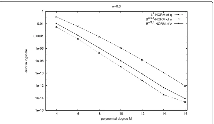
We first check the convergence behavior of numerical solutions with respect to the poly-nomial degreesM. In Figure , we plot the errors as functions of the polynomial degrees Mwithα= .,N= . Also, in Table , we list the maximum absolute errors ofq,u, and
Table 1 Maximum absolute errors forq,u, andJatN= 20,α= 0.3, and various choices ofM
for Example 5.1
M 4 6 8 10 12 14 16
q 4.08E–03 5.24E–05 2.93E–07 1.58E–09 9.97E–12 5.17E–14 2.30E–14
u 4.75E–02 7.96E–04 1.17E–05 1.39E–07 1.28E–09 9.82E–12 3.43E–13
J 2.86E–05 5.77E–09 8.23E–13 8.83E–17 6.38E–21 3.09E–25 1.12E–29
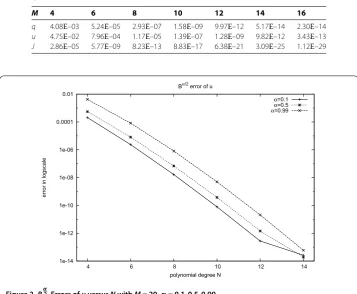
Figure 2 Bα2Errors ofu versus NwithM= 20,α= 0.1, 0.5, 0.99.
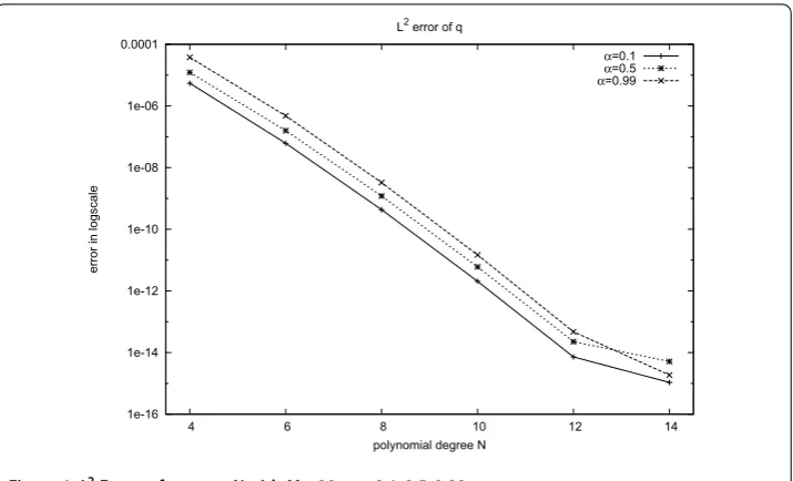
Figure 4 L2Errors ofq versus NwithM= 20,α= 0.1, 0.5, 0.99.
Table 2 Maximum absolute errors forq,u, andJatM= 20 and various choices ofαandNfor Example 5.1
Errors α N = 4 N = 6 N = 8 N = 10 N = 12 N = 14
q 0.1 7.11E–06 8.06E–08 6.19E–10 3.27E–12 1.79E–14 7.75E–15 0.5 1.68E–05 2.14E–07 1.61E–09 8.24E–12 2.94E–14 4.91E–16 0.99 6.96E–05 1.07E–06 8.98E–09 4.70E–11 1.63E–13 2.89E–16
u 0.1 7.74E–05 9.14E–07 7.45E–09 3.98E–11 2.14E–13 8.67E–14 0.5 1.82E–04 2.53E–06 1.97E–08 1.00E–10 3.66E–13 1.14E–14 0.99 6.69E–04 9.16E–06 7.07E–08 3.82E–10 1.75E–12 5.11E–15
J 0.1 8.39E–11 8.02E–15 3.24E–19 6.35E–24 6.76E–29 1.98E–31 0.5 4.64E–10 6.15E–13 3.01E–18 6.74E–23 7.83E–28 3.16E–32 0.99 5.00E–09 7.90E–13 3.88E–17 8.27E–22 9.04E–27 6.78E–32
J atα= .,N= , and various choices ofM. As expected, the errors show an expo-nential decay, since in this semi-log representation one observes that the error variations are essentially linear versus the degrees of polynomial.
We then investigate the temporal errors, which is more interesting to us because of the fractional derivative in time. In Figures to , we plot the errors as functions ofN with M= for three valuesα= ., ., .. The straight line of the error curves indicates that the convergence in time is also exponential. The maximum absolute errors ofq,u, andJatM= are also listed in Table .
Example . We choose another exact analytical solutions as
uq∗=sinπxet, zq∗=sinπx( –t)et, q∗= –zq∗.
Unlike the previous example which uses the exact solutionu(q∗) as the observation data, the observation datau(x,¯ t) here is calculated through (.) usingu(q∗) andz(q∗).
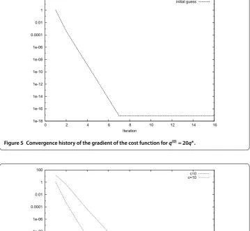
consider-Figure 5 Convergence history of the gradient of the cost function forq(0)= 20q∗.
Figure 6 Convergence history of the gradient of the cost function forq(0)=c.
ing q() = q∗. This represents a strong perturbation in the initial guess. We now fix M=N= ,α= .. In Figure , we plot the convergence history of the gradient of the objective function as a function of the iteration number withM=N= ,α= .. We see that the iterative method converges within seven iterations. We then takeq()to be constantcwithc= or , which has nothing to compare with the exact controlq∗. We repeat the same computation as in Figure . The result is given in Figure . These results seem to tell that the type and amplitude of the perturbation have no significant effects on the convergence of the optimization algorithm, since in any case the iterative algorithm converges with the same rate. In the following, the initial guess is set to .
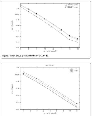
Figure 7 Errors ofu,z,q versus Mwithα= 0.6,N= 20.
Figure 8 Bα2Errors ofu versus NwithM= 20,α= 0.2, 0.6, 0.9.
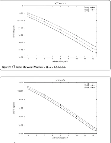
scale as a function of the polynomial degreesMandN, respectively. Also, in Tables and , we list the maximum absolute errors ofq,u, andJ. Clearly, all the errors show an exponential decay.
6 Concluding remarks
In the present work, we have shown an efficient optimization algorithm for the space-time fractional equation optimal control problem based on the spectral approximation. A priorierror estimates are derived. Some numerical experiments have been carried out to confirm the theoretical results.
Figure 9 Bα2Errors ofz versus NwithM= 20,α= 0.2, 0.6, 0.9.
Figure 10 L2Errors ofq versus NwithM= 20,α= 0.2, 0.6, 0.9.
Table 3 Maximum absolute errors forq,u, andJatN= 20,α= 0.6 and various choices ofM
for Example 5.2
M 4 6 8 10 12 14 16
q 7.24E–02 1.18E–03 1.62E–05 1.92E–07 1.75E–09 1.34E–11 1.57E–13
u 1.30E–01 2.17E–03 3.19E–05 3.78E–07 3.48E–09 2.66E–11 2.22E–13
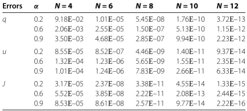
Table 4 Maximum absolute errors forq,u, andJatM= 20 and various choices ofαandNfor Example 5.2
Errors α N = 4 N = 6 N = 8 N = 10 N = 12
q 0.2 9.18E–02 1.01E–05 5.45E–08 1.76E–10 3.72E–13 0.6 2.06E–03 2.55E–05 1.50E–07 5.13E–10 1.15E–12 0.9 3.50E–03 4.68E–05 2.85E–07 9.94E–10 2.23E–12
u 0.2 8.55E–05 8.52E–07 4.46E–09 1.40E–11 9.37E–14 0.6 1.32E–04 1.23E–06 5.65E–09 1.55E–11 2.35E–14 0.9 1.01E–04 1.24E–06 7.83E–09 2.66E–11 6.33E–14
J 0.2 3.17E–05 2.37E–08 3.38E–11 4.55E–14 1.33E–15 0.6 5.52E–05 3.85E–08 2.22E–11 2.08E–13 2.44E–15 0.9 8.53E–05 8.61E–08 2.57E–11 9.77E–14 2.22E–16
terms of Riemann-Liouville derivatives. Secondly, studies for more complicated control problems and constraint sets are needed. Thirdly, although our analysis and algorithm are designed for the optimization of the distributed control problem, we hope that they are generalizable for the minimization problems of other parameters, such as boundary conditions and so on.
Competing interests
The authors declare that they have no competing interests.
Authors’ contributions
The authors have equal contributions to each part of this paper. All the authors read and approved the final manuscript.
Author details
1School of Science, Jimei University, Xiamen, 361021, China.2School of Mathematical Sciences, Xiamen University, Xiamen, 361005, China.
Acknowledgements
The work of Xingyang Ye is partially supported by the Science Foundation of Jimei University, China (Grant Nos. ZQ2013005 and ZC2013021), Foundation (Class B) of Fujian Educational Committee (Grant No. FB2013005), Foundation of Fujian Educational Committee (No. JA14180). The work of Chuanju Xu was partially supported by National NSF of China (Grant Nos. 11471274 and 11421110001).
Received: 8 January 2015 Accepted: 27 April 2015 References
1. Oustaloup, A: La Dérivation Non Entière: Théorie, Synthèse et Applications. Hermes, Paris (1995)
2. Zhang, H, Cao, JD, Jiang, W: Controllability criteria for linear fractional differential systems with state delay and impulses. J. Appl. Math.2013, Article ID 146010 (2013). doi:10.1155/2013/146010
3. Koeller, RC: Application of fractional calculus to the theory of viscoelasticity. J. Appl. Mech.51, 299-307 (1984) 4. Mainardi, F: Fractional diffusive waves in viscoelastic solids. In: Nonlinear Waves in Solids, pp. 93-97. ASME/AMR,
Fairfield (1995)
5. Bouchaud, JP, Georges, A: Anomalous diffusion in disordered media: statistical mechanisms, models and physical applications. Phys. Rep.195(4-5), 127-293 (1990)
6. Dentz, M, Cortis, A, Scher, H, Berkowitz, B: Time behavior of solute transport in heterogeneous media: transition from anomalous to normal transport. Adv. Water Resour.27(2), 155-173 (2004)
7. Goychuk, I, Heinsalu, E, Patriarca, M, Schmid, G, Hänggi, P: Current and universal scaling in anomalous transport. Phys. Rev. E73(2), 020101 (2006)
8. Benson, DA, Wheatcraft, SW, Meerschaert, MM: The fractional-order governing equation of Lévy motion. Water Resour. Res.36(6), 1413-1423 (2000)
9. Diethelm, K: The Analysis of Fractional Differential Equations. Springer, Berlin (2010)
10. Gutiérrez, RE, Rosário, JM, Machado, JT: Fractional order calculus: basic concepts and engineering applications. Math. Probl. Eng.2010, Article ID 375858 (2010). doi:10.1155/2010/375858
11. Miller, K, Ross, B: An Introduction to the Fractional Calculus and Fractional Differential Equations. Wiley, New York (1993)
12. Podlubny, I: Fractional Differential Equations. Academic Press, New York (1999)
13. Agrawal, O: A general formulation and solution scheme for fractional optimal control problems. Nonlinear Dyn.38(1), 323-337 (2004)
14. Frederico, G, Torres, D: Fractional conservation laws in optimal control theory. Nonlinear Dyn.53(3), 215-222 (2008) 15. Frederico, G, Torres, D: Fractional optimal control in the sense of Caputo and the fractional Noether’s theorem. Int.
16. Mophou, GM: Optimal control of fractional diffusion equation. Comput. Math. Appl.61(1), 68-78 (2011)
17. Dorville, R, Mophou, GM, Valmorin, VS: Optimal control of a nonhomogeneous Dirichlet boundary fractional diffusion equation. Comput. Math. Appl.62(3), 1472-1481 (2011)
18. Agrawal, OP, Hasan, MM, Tangpong, XW: A numerical scheme for a class of parametric problem of fractional variational calculus. J. Comput. Nonlinear Dyn.7(2), 021005 (2012)
19. Agrawal, O, Baleanu, D: A Hamiltonian formulation and a direct numerical scheme for fractional optimal control problems. J. Vib. Control13(9-10), 1269-1281 (2007)
20. Alipour, M, Rostamy, D, Baleanu, D: Solving multi-dimensional FOCPs with inequality constraint by BPs operational matrices. J. Vib. Control19(16), 2523-2540 (2013)
21. Baleanu, D, Defterli, O, Agrawal, O: A central difference numerical scheme for fractional optimal control problems. J. Vib. Control15(4), 583-597 (2009)
22. Bhrawy, A, Doha, E, Baleanu, D, Ezz-Eldien, S, Abdelkawy, M: An accurate numerical technique for solving fractional optimal control problems. Proc. Rom. Acad.16(1), 47-54 (2015)
23. Ezz-Eldien, S, Doha, E, Baleanu, D, Bhrawy, A: A numerical approach based on Legendre orthonormal polynomials for numerical solutions of fractional optimal control problems. J. Vib. Control (2015). doi:10.1177/1077546315573916 24. Liu, XY, Liu, ZH, Fu, X: Relaxation in nonconvex optimal control problems described by fractional differential
equations. J. Math. Anal. Appl.409(1), 446-458 (2014)
25. Li, XJ, Xu, CJ: A space-time spectral method for the time fractional diffusion equation. SIAM J. Numer. Anal.47(3), 2108-2131 (2009)
26. Li, XJ, Xu, CJ: The existence and uniqueness of the weak solution of the space-time fractional diffusion equation and a spectral method approximation. Commun. Comput. Phys.8(5), 1016-1051 (2010)
27. Lin, Y, Xu, C: Finite difference/spectral approximations for the time-fractional diffusion equation. J. Comput. Phys.
225(2), 1533-1552 (2007)
28. Bhrawy, A, Zaky, M, Baleanu, D: New numerical approximations for space-time fractional Burgers’ equations via a Legendre spectral-collocation method. Rom. Rep. Phys.67(2), 1-13 (2015)
29. Bhrawy, A, Al-Zahrani, A, Alhamed, Y, Baleanu, D: A new generalized Laguerre-Gauss collocation scheme for numerical solution of generalized fractional pantograph equations. Rom. J. Phys.59(7-8), 646-657 (2014)
30. Bhrawy, AH, Zaky, MA: A method based on the Jacobi tau approximation for solving multi-term time-space fractional partial differential equations. J. Comput. Phys.281, 876-895 (2015). doi:10.1016/j.jcp.2014.10.060
31. Lotfi, A, Yousefi, S, Dehghan, M: Numerical solution of a class of fractional optimal control problems via the Legendre orthonormal basis combined with the operational matrix and the Gauss quadrature rule. J. Comput. Appl. Math.250, 143-160 (2013)
32. Ye, X, Xu, C: A spectral method for optimal control problems governed by the time fractional diffusion equation with control constraints. In: Spectral and High Order Methods for Partial Differential Equations - ICOSAHOM 2012, pp. 403-414. Springer, Berlin (2014)
33. Doha, EH, Bhrawy, AH, Baleanu, D, Ezz-Eldien, SS, Hafez, RM: An efficient numerical scheme based on the shifted orthonormal Jacobi polynomials for solving fractional optimal control problems. Adv. Differ. Equ.2015, 15 (2015) 34. Adams, RA: Sobolev Spaces. Academic Press, New York (1975)