R E S E A R C H
Open Access
An exactly solvable multiple stochastic
optimal stopping problem
Hidekazu Yoshioka
1**Correspondence:
[email protected] 1Faculty of Life and Environmental
Science, Shimane University, Matsue, Japan
Abstract
A new kind of multiple stochastic optimal stopping problem is formulated and its associated recursive variational inequalities are derived. We show that these
variational inequalities can be solved exactly in a cascading manner. The relevance of the present problem in analyzing animal migration, which is an ecologically
important problem, is also briefly discussed.
Keywords: Multiple optimal stopping; Geometric Brownian motion; Dynamic programming principle; Variational inequality
1 Introduction
Stochastic optimal stopping models are useful mathematical tools for analyzing decision-making processes in the fields of financial [1, 2], environment [3, 4], and ecology [5–7]. Multiple optimal stopping problems based on stochastic differential equations (SDEs) are among the ones that have been analyzed most in detail because of their rich mathematical structures [8, 9]. Exactly solvable multiple optimal stopping models are useful from both theoretical and practical point of views [10, 11].
We are interested in solvability of a multiple optimal stopping problem that has not been focused on so far, which is related to animal migration: an important ecological problem. Our problem is explained below. In this paper, the summationki=jaiof a sequenceai
is replaced by 0 whenk<j. LetBt fort≥0 be a standard 1-D Brownian motion on the
probability space as in the usual setting [12]. Its associated completed filtration is denoted byF={Ft}t>0. Letτ0= 0. We consider a multiple optimal stopping problem of finding the
collection of the stopping timesτ = (τ1,τ2, . . . ,τM) (0 =τ0≤τ1≤τ2≤ · · · ≤τM, M≥1
is a given natural number) with no refraction. The stochastic processZt (t≥0) is the
geometric Brownian motion governed by the Itô SDE
dZt=Zt
r(t) dt+σ(t) dBt
, t> 0 (1)
with (r(t),σ(t)) = (ri,σi) forτi–1<t≤τiwhereri,σi> 0, 2ri>σi2 are given constants. We
putM+1(z) =z1–α/(1 –α) for the sake of brevity. The stopping times are chosen to
maxi-mize the performance index
Jτ(z) = E
M
i=1
ηi
τi
τi–1
qi
1 –βi
Z1–βi
s e–δi(s–τi–1)ds+ηM+1M+1(ZτM)
Z0=z (2)
with
ηi=e– i–1
j=1δj(τj–τj–1), (3)
where E is the expectation operator,δi> 0,qi> 0, and 0 <α<βM<βM–1<· · ·<β1< 1
are given constants andz≥0 is the initial condition ofZt. We show that an application
of the dynamic programming principle reduces the present optimal stopping problem to a series of variational inequalities (VIs). The VIs, and consequently the present multiple optimal stopping problem, turn out to be exactly solvable. Its implications in an ecological problem are briefly discussed as well.
The main difference between the present model and the existing models [8–11] is that the former has an ecological background, while the latter have the financial backgrounds. In addition, the performance indices to be maximized or minimized have different func-tional forms with each other. The resulting VIs have different forms as well. The main contribution of this paper is the derivation of an exact solution to the cascading system of VIs and its ecological implications.
By the strong Markov property of the processZt, (4) is rewritten as
(z) = sup
Similarly, introduce the functionsi(y) fory≥0 recursively as
i(y) = sup
The recursive equations (6) and (7) are later utilized to show that the present multiple optimal stopping problem results in a cascading system of VIs that can be solved in a cascading manner fromi=Mtoi= 1. The value functionis then obtained:(z) =1(z).
Assumei∈C1(0, +∞)∩C0([0, +∞)) for 1≤i≤Mand is twice continuously
elliptic operatorLiis defined as
for generic sufficiently smooth = (z). Then Theorem 10.4.1 [12] shows thati(1≤
i≤M) solves the VI
respectively. Theorem 1 is the main result of this paper, which shows that the VIs of the present multiple optimal stopping problem are exactly solvable.
Theorem 1 Assumeδi>riandλi> 0for1≤i≤M,and ki>ki+1for1≤i≤M– 1when
Proof of Theorem1 By (10), it is straightforward to check that the assumptionδi>rileads
toki> 1. General solutions ∈C2(0, +∞)∩C0([0, +∞)) to the problem
Li = 0, z> 0, (0) = 0 (13)
are expressed with a real constantcas (z) =czki. Fori=M, we have a candidate of the
solution of the form (12) withBM =qM/[λM(1 –βM)] whereBMz1–βM is the particular
solution toLMM–qMz1–βM/(1 –βM) = 0,z> 0. There are two unknowns,¯zM andAM,
which are determined from the smooth-pasting condition [13] atz=z¯M≥0:
The second equation of (14) excludes the case with¯zM= 0. Equation (14) is uniquely
solved as
AM=
βM–βM+1
1 –βM
(¯zM)–(kM–1+βM+1)
kM– 1 +βM
> 0,
¯
zM=
1 –βM+1
1 –βM
kM– 1 +βM
kM– 1 +βM+1
qM
λM
1
βM–βM+1 > 0.
(15)
Uniqueness of the solutionMto VI (9) in a viscosity sense follows from an infinite
hori-zon counterpart of Theorem 3.1 [14]. Regularity conditionsM∈C1(0, +∞)∩C0([0, +∞))
andM ∈C2(0,z¯M)∩C2(z¯M, +∞) directly follow from the form ofM. Hence, M =
M(z) is twice continuously differentiable almost everywhere forz> 0.
The discussion above can be continued for 1≤i≤M– 1 withM≥2. The proof in what follows is based on a recursive argument. We firstly assume 0 <z¯1<¯z2<· · ·<z¯M < +∞
and later show that this assumption is satisfied by appropriately choosing the sequence 0 <q1<q2<· · ·<qM< +∞. Assume that the statement of the theorem is true for alljsuch
thati+ 1≤j≤M. Then, from VI (9), we find that the candidate of its solution is expressed as (12) withBi=qi/[λi(1 –βi)] whereBiz1–βiis the particular solution toLii–qiz1–βi/(1 –
βi) = 0,z> 0. As in the case fori=M, there are two unknownsz¯iandAiin (12). They are
determined from the smooth-pasting condition atz=z¯i≥0:
Aizki+Biz1–βi=Ai+1zki+1+Bi+1z1–βi+1,
Aikizki–1+Bi(1 –βi)z–βi=Ai+1ki+1zki+1–1+Bi+1(1 –βi+1)z–βi+1, z=z¯i<z¯i+1.
(16)
The second equation of (14) excludes the case withz¯i= 0. A remarkable difference
be-tween the cases withi<Mandi=Mis thatz¯i andAicannot be expressed explicitly in
general in the former case. Fortunately, they are uniquely found from (16) as shown below. Combining the two equations of (16) leads to the equation to be solved byz¯i:
Bi(ki– 1 +βi) =fi(z), (17)
wherefi(z) forz≥0 is the polynomial
fi(z) =Ai+1(ki–ki+1)zki+1–1+βi+Bi+1(ki– 1 +βi)zβi–βi+1. (18)
The left-hand side of (17) and all the coefficients and powers appearing infiare
posi-tive by the assumption of the theorem. In addition,fi(z) is monotonically increasing with
respect toz> 0,limz→+∞fi(z)→+∞, andfi(0) = 0. Therefore, Eq. (17) admits a unique
positive solution by the classical intermediate theorem: namely,z¯i> 0. Substituting thisz¯i
into (16) uniquely yieldsAi. A useful result onfiis that
z<¯zi(z>z¯i) when Bi(ki– 1 +βi) >fi(z)
Bi(ki– 1 +βi) <fi(z)
(19)
due to its monotonicity. The sign ofAiis positive as shown in what follows. Combining
the two equations of (16) yields
wheregi(z) forz≥0 is defined as
gi(z) =Bi(ki+1– 1 +βi)z1–βi–Bi+1(ki+1– 1 +βi+1)z1–βi+1. (21)
By (20) and the assumptions of the theorem,Ai> 0 ifgi(¯zi) > 0. Define˜zi> 0 as
˜
zi=
Bi(ki+1– 1 +βi)
Bi+1(ki+1– 1 +βi+1)
1
βi–βi+1
, (22)
which is the unique solution togi(z) = 0 forz> 0. By the functional form ofgi,gi(z) < 0 for
z>z˜i. Thus,Ai> 0 ifz¯i<z˜i.
By (19),z¯i<˜ziwhenBi(ki– 1 +βi) <fi(z˜i). The quantityfi(˜zi) is calculated as
fi(˜zi) =Ai+1(ki–ki+1)z˜ki+1–1+
βi
i +Bi+1(ki– 1 +βi)z˜
βi–βi+1
i
=Ai+1(ki–ki+1)z˜kii+1–1+βi+Bi
(ki– 1 +βi+1)(ki+1– 1 +βi)
ki+1– 1 +βi+1
. (23)
Definelias
li=ki– 1 +βi–
(ki– 1 +βi+1)(ki+1– 1 +βi)
ki+1– 1 +βi+1
. (24)
By (24), the right-hand side of (23) is positive. A straightforward calculation shows
(ki+1– 1 +βi+1)li= (ki– 1 +βi)(ki+1– 1 +βi+1) – (ki– 1 +βi+1)(ki+1– 1 +βi)
= (ki+1–ki)(βi–βi+1)
< 0, (25)
namely, the desired inequality
li< 0 (26)
sinceki>ki+1andβi>βi+1. The inequalityBi(ki– 1 +βi) <fi(z˜i) follows from (26).
There-fore, we havez¯i<z˜iand thusAi> 0.
Uniqueness of the solutioni∈C1(0, +∞)∩C0([0, +∞)) is then proven as follows. In
addition,i=i(z) is identified withi+1=i+1(z) forz>z¯iby the construction, meaning
thatiis twice continuously differentiable except at theM–i+ 1 pointsz¯i,¯zi+1, . . . ,¯zM.
Furthermore, uniqueness of the solutionito VI (9) in a viscosity sense follows from an
infinite horizon counterpart of Theorem 3.1 [14]. Therefore, by the induction, it is shown that the statement of the theorem is true if we can construct a sequence 0 <z¯1<z¯2<· · ·< ¯
zM< +∞. This issue is not encountered forM= 1 where the problem involves a single
optimal stopping time, since we have 0 <z¯1< +∞.
AssumeM≥2. By the second equation of (15),z¯Mcan be seen as an increasing power
function ofqM. In addition,BM is increasing with respect toqM. Therefore, for a fixed
qM–1, it is possible to choose a sufficiently largeqMsuch that
This inequality means that there existz¯M–1and¯zMwith 0 <z¯M–1<z¯M< +∞by
appro-priately choosingqM–1andqM. As a next step, assumeM= 3 for the sake of simplicity. The
argument below can straightforwardly be extended toM≥3. Assume that the condition 0 <z¯2<z¯3< +∞is satisfied. The explicit expression ofz¯1is not available, but it satisfies
lim
q1→+0¯
z1= 0. (28)
Actually, (17) and (18) withi= 1 show that the left-hand side of (17) is increasing with respect toq1, while the right-hand side of (17) is independent ofq1. Therefore, we can
choose a sufficiently smallq1> 0 such thatB1(k1– 1 +β1) <f1(¯z2); namely, 0 <z¯1<z¯2. We
then have 0 <z¯1<z¯2<z¯3< +∞. The proof forM≥3 is essentially the same.
The following proposition is proven in an essentially similar way with Theorem 1.
Proposition 2 Replace “ki>ki+1 for1≤i≤M– 1when M≥2” by “ki=ki+1for1≤i≤
M– 1when M≥2” in Theorem1.Then we havei(1≤i≤M)of the form(12)where
Ai=
βi–βi+1
1 –βi
(z¯i)–(ki–1+βi+1)
ki– 1 +βi
> 0 and z¯i=
1 –βi+1
1 –βi
ki– 1 +βi+1
ki– 1 +βi
λi+1qi
λiqi+1
1
βi–βi+1
. (29)
The second equation of (29) shows thatz¯i is expressed as a monotonically increasing
and unbounded function ofqi/qi+1, implying thatz¯M–1<z¯MifqMis sufficiently larger than
qM–1. Similarly, we havez¯M–2<z¯M–1ifqM–1is sufficiently larger thanqM–2. We can choose
largerqMif necessary. SinceMis bounded, we can construct a sequence 0 <q1<q2<· · ·<
qM< +∞such that 0 <¯z1<z¯2<· · ·<z¯M< +∞.
An immediate consequence of Theorem 1 and Proposition 2 is the next proposition.
Proposition 3 1is the value functionunder the assumption of Theorem1or that of
Proposition2.
Remark4 A numerical example of Theorem 1 is provided. Set the following parameter values:δ1= 6.5,δ2= 4,r1= 3,r2= 2,σ1= 0.5,σ2= 0.2,β1= 0.8,β2= 0.5,β3= 0.1,q1= 0.4,
andq2= 0.9. In this case, the growth rateriof the animal population increases while its
fluctuationσidecreases asiincreases, which is an ecologically reasonable situation. Based
on these parameter values, we havek1= 2.074 >k2= 1.981,λ1= 5.920, andλ2= 3.005.
These given and calculated constants comply with the assumption of Theorem 1. Fur-thermore, we haveA1= 1.393,A2= 1.224,B1= 0.338,B2= 0.599,B3= 1.111,z¯1= 0.145,
andz¯2= 0.469. The obtained results satisfy 0 <z¯1<¯z2andA1,A2> 0, which comply with
the results of Theorem 1.
Remark5 Each optimalτiis denotedτi∗. Under the assumption of Theorem 1 or that of
Proposition 2, the optimal stopping timeτi∗is expressed as
τi∗=infτ|τ>τi–1∗ ,Zτ=z¯i
for 1≤i≤M,τ0∗= 0. (30)
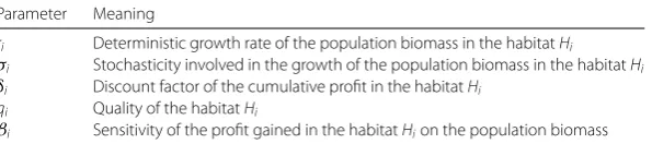
Table 1 Meaning of the variables and parameters of the present multiple optimal stopping problem in analyzing fish migration
Parameter Meaning
ri Deterministic growth rate of the population biomass in the habitatHi
σi Stochasticity involved in the growth of the population biomass in the habitatHi
δi Discount factor of the cumulative profit in the habitatHi
qi Quality of the habitatHi
βi Sensitivity of the profit gained in the habitatHion the population biomass
a straightforward calculation gives
where the notationz¯0=zis employed for the sake of simplicity. Similarly, the variance of
τMis found as
The present multiple optimal stopping problem is a simple theoretical model for mi-gration of animals, migratory fishes in particular [16]. A single optimal stopping problem for analyzing animal migration between two habitats has been discussed in Yoshioka and Yaegashi [7] from a numerical viewpoint. Assume that there areM+ 1 habitats, which are denotedH0,H1, . . . ,HMwhereH0is the initial habitat andHMis the final habitat: the goal
of the migration. The stochastic processZtrepresents the biomass of an animal population
at the timet. The stopping timeτirepresents the time to move fromHi–1toHi. The
objec-tive of the animal population is to choose the sequence of stopping timesτi(1≤i≤M),
so that the sum of the cumulative profit gain in each habitatHi(0≤i≤M– 1) and the
terminal wealth gained at the goal of migrationHM, namely the performance indexJτ in
(2), is maximized.
An example is the migratory fishPlecoglossus altivelis(P. altivelis, Ayu) having an annual life cycle that migrates between a river and the seas [17]. The present mathematical model can be applied to modelling one-generation life history of the fish withM= 2. In each autumn, the adults spawn eggs in downstream reaches of a river in which they live and die soon afterward. Hatched larvae descend to coastal areas of a downstream water body of the river: the sea or an estuary (H0). In the coming spring, grown fishes ascend into
the midstream of the river to mature (H1) until the coming autumn. In the autumn, the
fishes descend to the downstream reach of the river where they can spawn (H2). Table 1
summarizes the meaning of the model parameters in the above-mentioned problem. The assumptionsδi>riandλi> 0 for 1≤i≤Mandki>ki+1 for 1≤i≤M– 1 when
habitat quality degrades as the time elapses. This is in accordance with the fact that animal migration is often driven by seasonal changes of habitat quality. The remaining condition
ki>ki+1is satisfied ifδiis sufficiently larger thanδi+1. For the animal migration, this
con-dition to the situation where degradation of the habitat quality is critical for the earlier period of the animal life history.
4 Conclusions
This paper focused on a solvable multiple optimal stopping problem related to animal mi-gration. An extension of the present problem is to consider a refractionτi+1–τi≥μi> 0,
which leads to a different system of VIs, and consequently different value functions and optimal stopping criteria. Solvability of the problem with a refraction is currently under investigation for more realistic mathematical modelling of animal migration. There exist recent studies on optimization models of ecological and biological systems involving de-lays [18–20]. These systems are clearly more complicated than the system focused on in this paper. To examine the applicability of the present methodology, to extend these mod-els will be a quite interesting topic. Applicability of the present formalism to real animal migration, which is based on a mixed control problem like those in Koo et al. [21] and Lee and Shin [22], is also currently in progress.
Acknowledgements
JSPS Research Grant No. 17K15345 and a grant to Shimane University Fisheries Management Research Center from the Ministry of Land, Infrastructure, Transport and Tourism of Japan support this research. The author thanks the two Reviewers for their valuable comments and suggestions. The author also thanks Mr. Yuta Yaegashi of Graduate School of Agriculture, Kyoto University for his careful check on Grammar and Style of the manuscript.
Funding
JSPS Research Grant No. 17K15345 supports this research. A grant to Shimane University Fisheries Management Research Center from the Ministry of Land, Infrastructure, Transport and Tourism of Japan.
List of abbreviations
VI(s), Variational inequality(ies).
Availability of data and materials
All the data are provided in the manuscript.
Competing interests
The author declares that he has no competing interests.
Authors’ contributions
HY carried out mathematical analysis and wrote the manuscript. Author read and approved the final manuscript.
Publisher’s Note
Springer Nature remains neutral with regard to jurisdictional claims in published maps and institutional affiliations.
Received: 17 October 2017 Accepted: 2 May 2018 References
1. Jacka, S.L.: Optimal stopping and the American put. Math. Finance1, 1–14 (1991). https://doi.org/10.1111/j.1467-9965.1991.tb00007.x
2. Zhu, S.P., Le, N.T., Chen, W., Lu, X.: Pricing Parisian down-and-in options. Appl. Math. Lett.43, 19–24 (2015). https://doi.org/10.1016/j.aml.2014.10.019
3. Pindyck, R.S.: Optimal timing problems in environmental economics. J. Econ. Dyn. Control26, 1677–1697 (2002). https://doi.org/10.1016/S0165-1889(01)00090-2
4. Framstad, N.C., Strand, J.: Energy intensive infrastructure investments with retrofits in continuous time: effects of uncertainty on energy use and carbon emissions. Resour. Energy Econ.41, 1–18 (2015).
https://doi.org/10.1016/j.reseneeco.2015.03.003
5. Reed, W.J.: The decision to conserve or harvest old-growth forest. Ecol. Econ.8, 45–69 (1993). https://doi.org/10.1016/0921-8009(93)90030-A
7. Yoshioka, Y., Yaegashi, Y.: Numerical simulation of animal migration via a nonlinear degenerate elliptic free boundary problem. In: Proceedings of the 36th JSST Annual International Conference on Simulation Technology. Proceedings, pp. 174–177 (2017)
8. Carmona, R., Dayanik, S.: Optimal multiple stopping of linear diffusions. Math. Oper. Res.33, 446–460 (2008). https://doi.org/10.1287/moor.1070.0301
9. Carmona, R., Touzi, N.: Optimal multiple stopping and valuation of swing options. Math. Finance18, 239–268 (2008). https://doi.org/10.1111/j.1467-9965.2007.00331.x
10. Cai, N., Sun, L.: Valuation of stock loans with jump risk. J. Econ. Dyn. Control40, 213–241 (2014). https://doi.org/10.1016/j.jedc.2014.01.004
11. Dai, M., Kwok, Y.K.: Optimal multiple stopping models of reload options and shout options. J. Econ. Dyn. Control32, 2269–2290 (2008). https://doi.org/10.1016/j.jedc.2007.10.002
12. Øksendal, B.: Stochastic Differential Equations. Springer, Berlin (2003)
13. Dixit, A.K., Pindyck, R.S.: Investment Under Uncertainty. Princeton University Press, Princeton (1994) 14. Reikvam, K.: Viscosity solutions of optimal stopping problems. Stoch. Stoch. Rep.62, 285–301 (1998).
https://doi.org/10.1080/17442509808834137
15. Zhang, L., Du, Z.: On the reflected geometric Brownian motion with two barriers. Intell. Inform. Manag.2, 295–298 (2010). https://doi.org/10.4236/iim.2010.23034
16. Zydlewski, J., Wilkie, M.P.: Freshwater to seawater transitions in migratory fishes. Fish Physiol.32, 253–326 (2013). https://doi.org/10.1016/B978-0-12-396951-4.00006-2
17. Yaegashi, Y., Yoshioka, H., Unami, K., Fujihara, M.: An optimal management strategy for stochastic population dynamics of releasedPlecoglossus altivelisin rivers. Int. J. Model. Sim. Sci. Comput.8, 1750039 (2017). https://doi.org/10.1142/S1793962317500398
18. Liu, L., Meng, X.: Optimal harvesting control and dynamics of two-species stochastic model with delays. Adv. Differ. Equ.2017, 18 (2017). https://doi.org/10.1186/s13662-017-1077-6
19. Feng, T., Meng, X., Liu, L., Gao, S.: Application of inequalities technique to dynamics analysis of a stochastic eco-epidemiology model. J. Inequal. Appl.2016, 327 (2016). https://doi.org/10.1186/s13660-016-1265-z 20. Leng, X., Feng, T., Meng, X.: Stochastic inequalities and applications to dynamics analysis of a novel SIVS epidemic
model with jumps. J. Inequal. Appl.2017, 138 (2017). https://doi.org/10.1186/s13660-017-1418-8
21. Koo, J.L., Koo, B.L., Shin, Y.H.: An optimal investment, consumption, leisure, and voluntary retirement problem with Cobb–Douglas utility: dynamic programming approaches. Appl. Math. Lett.26, 481–486 (2013).
https://doi.org/10.1016/j.aml.2012.11.012
22. Lee, H.S., Shin, Y.H.: An optimal investment, consumption-leisure and voluntary retirement choice problem with subsistence consumption constraints. Jpn. J. Ind. Appl. Math.33, 297–320 (2016).