R E S E A R C H
Open Access
On the numerical solution of Fisher’s
equation with coefficient of diffusion term
much smaller than coefficient of reaction
term
K.M. Agbavon
1, A.R. Appadu
1*and M. Khumalo
2*Correspondence: [email protected]; [email protected]
1Department of Mathematics and
Applied Mathematics, University of Pretoria, Pretoria, South Africa Full list of author information is available at the end of the article
Abstract
Li et al. (SIAM J. Sci. Comput. 20:719–738,1998) used the moving mesh partial differential equation (MMPDE) to solve a scaled Fisher’s equation and the initial condition consisting of an exponential function. The results obtained are not accurate because MMPDE is based on a familiar arc-length or curvature monitor function. Qiu and Sloan (J. Comput. Phys. 146:726–746,1998) constructed a suitable monitor function called modified monitor function and used it with the moving mesh differential algebraic equation (MMDAE) method to solve the same problem of scaled Fisher’s equation and obtained better results.
In this work, we use the forward in time central space (FTCS) scheme and the nonstandard finite difference (NSFD) scheme, and we find that the temporal step size must be very small to obtain accurate results. This causes the computational time to be long if the domain is large. We use two techniques to modify these two schemes either by introducing artificial viscosity or using the approach of Ruxun et al. (Int. J. Numer. Methods Fluids 31:523–533,1999). These techniques are efficient and give accurate results with a larger temporal step size. We prove that these four methods are consistent for partial differential equations, and we also obtain the region of stability.
Keywords: Fisher’s equation; Moving mesh method; FTCS; NSFD; Artificial viscosity
1 Introduction
Real-life problems are mainly modeled by partial differential equations (PDEs) with ap-plications to engineering, physics, chemistry, ecology, biology, and other related fields of science. PDEs can be of different forms:
(i) linear or nonlinear,
(ii) homogeneous or nonhomogeneous, (iii) elliptic, hyperbolic, or parabolic.
PDEs have some specifications that give the information how smooth the solution is, how rapid information propagates, and what is the impact of initial and boundary conditions (which help to find if a particular approach is suitable to the problem being portrayed by the PDEs). Some examples of modeling real-life problems can be found in [4–7]. Indeed,
a new model and solution method for wave propagation in compressible two-phase flow problem were proposed by Zeidan et al. [4]. The model consists of six equations and is applicable for pure fluid and fluid mixtures. A modern shock-capturing method (total-variation diminishing (TVD)) slope limiter centered scheme (SLIC)) has been proposed to solve the problems considered in simple way and with good accuracy. The modeling of a two-phase gas–magma mixture was made using total-variation diminishing (TVD) slope limiter centered scheme (SLIC) and the model is based on a nonhomogeneous system of nonlinear hyperbolic conservation laws [5]. There is strong evidence that the model and the method used are accurate, robust, and conservative. The study of unsteady cavitation in liquid hydrogen flows was made in the context of compressible two-phase one-fluid inviscid solver by Goncalvés and Zeidan [6]. Three conservation laws for mixture mass, mixture momentum, and total energy alongside with gas volume fraction transport equa-tion with thermodynamic effect were used. Minhajul et al. [7] investigated the interaction of weak shocks for widely used isentropic drift-flux equations of two-phase flows. The existence and uniqueness condition for elementary waves was obtained.
Our study is based on reaction–diffusion equations of the form of PDEs, which are mostly used in modeling transport of air, adsorption of pollutants in soil, diffusion of neutrons, food processing, modeling of biological and ecological systems, modeling of semiconductors, oil reservoir flow transport, among others [8]. Some tangible applica-tions are modeling amazing patterns and phenomena such as tree–grass interacapplica-tions in fire-prone savannas [9], pulse splitting and shedding (the Gray–Scott equation; see [10]). The Gray–Scott equation has some applications, namely, reaction and competition in ex-citable systems, autocatalysis, reaction between two chemical species with different diffu-sivities [11], modeling labyrinthine patterns [12], which are formed in models of catalytic reactions. There are only a few cases where analytical solutions to such reaction–diffusion equations exist, and therefore we need to construct accurate and efficient numerical meth-ods.
In this work, our interest is in Fisher’s equation [13], which describes spontaneous growth and spread of a dominant gene. Fisher considers a population that is distributed linearly in an habitat (shore line) with uniform density. If the mutation happens at any point of the habitat, then the mutant gene is expected to increase at the risk of the allelo-morphs previously occupying the same position. This occurrence will be first terminated in a neighborhood of the mutation and later in the adjacent portion of its range. Assuming the range to be long enough in comparison with the distance separating the locations of offspring from those of their parents, there will be from the origin a wave of increase in the gene frequency.
1.1 Background of Fisher’s equation
We consider Fisher’s equation [13]
ut=uxx+u(1 –u), (1)
wherex∈(–∞, +∞),t> 0, and the boundary and initial conditions are
lim
x→–∞u(x,t) = 1, x→lim+∞u(x,t) = 0, (2)
This problem [13] was solved by Kolmogorov et al. [14] by introducing the concepts of traveling waves and the existence of wave speedc. Moreover, they showed that the propa-gation speedcof the waves is greater than two (c≥2) if the initial conditionu0(x) is in the
interval [0, 1] and the type of solution isu(x,t) =v(ξ), whereξ=x–ctsatisfyingu∈[0, 1] for all ξ. They also proved that such solutions do not exist forc∈[0, 1). The studies in [15] showed that all positive initial data,u0(x), decaying at least exponentially asx→ ∞
evolves to a unique travelling wave. If
u0(x)∼e–β asx→ ∞, (4)
then the solutionuevolves a traveling wave speed, which is a function ofβ, where
c(β) =
⎧ ⎨ ⎩
β+1β, β≤1,
2, β≥1. (5)
Furthermore, they proved that if the initial amplitude drops sufficiently quickly asxgoes to infinity, then the propagation speed of the wave (which determines the behavior of initial condition) has the minimum value,c= 2.
The numerical implementation of Eq. (1) with boundary and initial conditions given, respectively, by (2) and (3) involving the traveling wave solution is challenging due to the dependence of sensitive solution on the initial data behavior at infinity. For instance, prob-lem (1) with initial condition (3) (Cauchy problem) is replaced by an initial and boundary value problem on the finite spatial domain [xl,xr]. Moreover, Gazdag and Canosa [16] re-solved this issue by imposing an asymptotic representation of the boundary condition (2) atx=xl,x=xr. They found that the solution draws toward a traveling wave of the min-imum speedc= 2. They concluded that the demanding time to change to the minimum wave speed profile is linked to the right-hand cutoff pointx=xr. The same approach was done by Hagstrom et al. [15] with the wave speed greater than the minimum wave speed
c= 2. They showed that the traveling wave solutions can be interpreted in finite domain by constructing accurately the asymptotic boundary conditions atx=xlandx=xr. They obtained good results withu(xl,t) = 1 andu(xr,t) = 0 fort≥0.
Many authors like Canosa [17] and Hagstrom and Keller [15] have worked on the issue of stability and sensitivity of the solution to the boundary of traveling wave. For instance, the equilibrium solutionsu= 0 andu= 1 of Eq. (1) are, respectively, unstable and stable to small perturbations. Moreover, they demonstrated that all traveling waves are stable to small perturbations of compact support but unstable to those of infinite support.
In 2005, Anguelov et al. [18] solved the same problem (Eq. (1)) by using a periodic initial condition withθ-nonstandard method. They concluded that their method is elementarily stable in the limit case of space-independent variable, stable with respect to the bounded-ness and positivity property, and finally stable with respect to the conservation of energy in the stationary case.
2 Organization of paper
and FTCS-difference scheme are studied, and numerical results are displayed. Sections7
and8are devoted to derivation and properties of NSFD and NSFD-schemes, and results are presented. In Sect.9, we add artificial viscosity to both FTCS and NSFD and study properties of new schemes and present some results. In Sect.10, we highlight the salient features of this paper. All simulations are performed using MATLAB R2014a software on an Intel core2 as CPU.
3 Moving mesh method
Li et al. [1] have considered the scaled Fisher equation
ut=uxx+ρu(1 –u), (6)
wherex∈(–∞, +∞),t> 0, andρ is a positive large constant. The boundary condition and initial condition are given by Eqs. (2) and (3), respectively. The exact solution to this problem is
u(x,t) =
1 +exp
ρ
6x– 5ρ
6 t
–2
, (7)
with wave speedc= 5√ρ/6 and the minimum wave speedc= 2√ρ. Li et al. [1] used the method called the moving mesh partial differential equation (MMPDE). They obtained poor results whenρwas chosen to be 104and concluded that MMPDE is not suitable for
reaction–diffusion equation (in particular, Fisher’s equation) when the reaction term is much greater than the diffusion term with initial condition consisting of an exponential function. This is due to the fact that MMPDE is based on familiar arc-length or curvature monitor function and does not produce accurate results [19]. Qiu et al. [2] improved the results of Li et al. [1] by constructing a specific monitor function and used the method of moving mesh differential algebraic equation (MMDAE).
The technique of the MMPDE method has been utilized broadly over the last few years to find a solution to time-dependent partial differential equations (PDEs). The method consists of moving the mesh points as time change with motion designed to minimize some measurement in computational error [2].
We consider the variablesζ andtwithζ defined by a one-to-one coordinate transfor-mation of the form
x=x(ζ,t), ζi= 1 + 2i
N, i= 0, . . . ,N, (8)
whereζiare spaced nodes in the interval [–1, 1] to the nodes{xi}iN=0in the interval [xl,xr], with
xl=x0(t) <x1(t) <· · ·<xN(t) =xr, ∀t≥0.
We can rewrite (6) in a semidiscrete form such that
˙
ui–x˙i
ui+1–ui–1 xi+1–xi–1
= 2
xi+1–xi–1
ui+1–ui
xi+1–xi
–ui–ui–1
xi–xi–1
fori= 1, 2, . . . ,N– 1 by using the Lagrangian form [19]
˙
u–x˙∂ux=∂uxx+ρu(1 –u). (10)
Moreover u˙,x˙ are the derivatives respect tot, independent ofζ, and{xi}Ni=0 and{ui}Ni=0
are the time-dependent vectors for approximations. To adjust the mesh to the solution as presented in [20], they introduced the equidistribution principle
x(ζ,t)
xl
M(s,t)ds=ζ x(xr)
xl
M(s,t)ds, (11)
whereM> 0 indicates the monitor function that has to be equally distributed between the nodesxl,xr. Differentiation of Eq. (11) with respect toζ gives
∂ζ
Mx(ζ,t)∂ζx(ζ,t)
= 0. (12)
Furthermore, Eq. (12) has been used in [20] to derive a collection of moving meshs, and the most accurate of this collection is [21]
∂ζ ζx˙= –
1
τ∂ζ(M∂ζx), (13)
denoted by MMPDE6 with small positive parameterτ1. Under the condition that the discretization has been done on the gridζiand using the second-order central differences leads to a semidiscrete form of moving mesh equation:
˙
xi–1– 2˙xi+x˙i+1= –
1
τ
Mi+1/2(xi+1–xi) –Mi+1/2(xi–xi–1)
(14)
fori= 1, 2, . . . ,N– 1 withM
i+12 being a smoothed monitor function given in [19,20] by
M
i+12 =
i+p
k=i–pM2k+1/2( q q+1)|k
–i|
i+p k=i–p(
q q+1)|k–i|
, (15)
whereqis a positive real number, andpis a nonnegative integer. Furthermore, setting
Mi+1/2(xi+1–xi) –Mi+1/2(xi–xi–1) = 0 (16)
in Eq. (14) leads to the moving mesh differential-algebraic equation (MMDAE) developed by Mulholland et al. [19]. This method combines systems (9) and (16). The difference be-tween MMPDE6 and MMDAE is that MMPDE6 accommodates the parameterτ, which shows the time used to attain equidistribution from some initial state, whereas MMDAE enforces the approximate equidistribution condition (16) at each moment of time in the time discretization.
Each problem has its own choice of a monitor function. This makes the choice of a mon-itor function an open question. Following [2,19,20], the monitor function (arc-length) is defined by
M(x,t) =1 +α2(∂
with its discrete approximationMi+1/2being
Mi+1 2 =
1 +α2
ui+1–ui
xi+1–xi
2
, (18)
where the parameterα measures the amplitude to which the solution slope has control over the mesh location.
It has been shown in [2] that moving mesh based on the arc-length and curvature mon-itor function is not convenient for the computational solution of Eq. (6). Indeed, firstly, the computed solution att= 2.5×10⁻³is susceptible to the choice ofτ (at values 10–3,
10–5, 10–7 withαfixed at 2 andx
l= –0.2,xr= 0.8) in Eq. (13) in the moving mesh using the arc-length monitor function. Secondly, in the common monitor function utilized, the first derivative in (17) is substituted by the second derivative, and we have
M(x,t) =1 +α2(∂xxu)2
1/4
(19)
with its discrete approximation
M4i+1 2 = 1 +
α2
1
xi+1–xi
ui+2–ui
xi+2–xi
–ui+1–ui–1
xi+1–xi–1 2
. (20)
The results show the same sensitivity as in the case of arc-length monitor function. There is oscillation of the solution at the front of wave. In the quest for obtaining the accurate result, Qiu et al. [2] introduced the modified monitor function.
3.1 Modified monitor function
The modified monitor function is constructed to give a great nodal density and hence a better accuracy at the wave front. It has been shown by Hagstrom and Keller [15] and Gazdag and Canosa [16] that the difficulties that occur in simulating numerically the trav-eling waves for Fisher’s equation come from the front of the wave. This is why significant care should be taken in formulation of boundary conditions atx=xr. Furthermore, the results in [16] showed that the numerical solution of all traveling wave are stable to small disturbances with compact support and unstable with infinite extent especially to trunca-tion errors inserted at the wave front. Consequently, it is an origin of inaccuracy of trun-cations errors rather than similar truntrun-cations errors introduced at the back of the wave. In this regard, the modified monitor function is
M(x,t) =1 +α2(1 –u)2+β2(a–u)2(uxx)2
1/2
, (21)
whereα,β, andaare real specific carefully chosen parameters. The expressions (1 –u)2
and (a–u)2are designed to give more influence of the curvature region at the front of the
wave than that of the corresponding curvature region at the back of the wave.
Withα= 1.5,β= 0.1,a= 1.015, andt= 2.5×10⁻³in the computations of MMDAE and
the modified monitor function given by Eq. (21), the maximum pointwise error 9.25×10⁻³
Table 1 Computation ofL1andL∞errors using MMPDE and MMDAE methods with
ρ= 104,α= 1.5,β= 0.1,a= 1.015,τ= 10–7,N= 50, at timet= 2.5×10⁻³
Methods L1error L∞error CPU
MMPDE O(1) 4.29×10⁻² ext
MMDAE 9.25×10–3 k×10–2 0.86ext
with the parameterτ = 10–7 and timet= 2.5×10⁻³, theL
∞ error is 4.29×10⁻². For the values greater than N= 50 withτ = 10–7 and timet= 2.5×10⁻³, the error is not diminished. Whenever the reduction is applied to the value ofτ, we have the reduction in theL∞error.L1andL∞errors for MMPDE and MMDAE are displayed in Table1.
4 Numerical experiments
We consider two problems. Firstly, we consider the same problem as in Qiu et al. [2], which involves solving the following:
Problem 1
ut=uxx+ 104u(1 –u)
forx∈[–0.2, 0.8]with boundary conditionslimx→–∞u(x,t) = 1and
limx→+∞u(x,t) = 0and time2.5×10–3.
The initial condition is
u(x, 0) =
1 +exp
ρ
6x
–2
. (22)
Secondly, we consider a slight modification of Problem 1. We use a larger domain with the same boundary and initial conditions and the same propagation time.
Problem 2
ut=uxx+ 104u(1 –u)
forx∈[–10, 90]with boundary conditionslimx→–∞u(x,t) = 1andlimx→+∞u(x,t) = 0 and time2.5×10–3.
The initial condition is
u(x, 0) =
1 +exp
ρ
6x
–2
. (23)
In the next sections, we present the numerical methods used and study the properties.
5 Forward in time central space (FTCS)
The forward in time central space (FTCS) scheme, when used to discretize Eq. (6), gives [22]
un+1 m –unm
k =
unm+1– 2un m+unm–1
h2 +ρu
n m
1 –unm. (24)
A single expression for the FTCS scheme is
where R= hk2. The time-step size and spatial mesh are denoted by k and h, respec-tively.
5.1 Stability
Equation (6) is nonlinear, and hence Fourier series stability analysis cannot be applied di-rectly. We need to freeze the coefficients before applying von Neumann stability analysis [23]. Taha and Ablowitz [24] obtained the stability of a method proposed by Zabusky and Krustal [25] for Korteweg–de Vries (KdV) equation using the method of freezing coeffi-cients and von Neumann stability analysis. The scheme derived by Zabusky and Kuskal for the KdV equationut+ 6uux+uxxx= 0 is
To obtain stability, Taha and Ablowitz [24] expressuuxasumaxuxand use the ansatzunm=
ξneImw, wherewis the phase angle. They obtain the following equation:
ξ–ξ–1
which can be rewritten as
ξ=ξ–1–12k|umax|
The linear stability requirement is
k
Appadu et al. [26] used the method of freezing coefficient and von Neumann stability analysis to obtain the region of stability of some schemes for Eq. (6). We use the same idea to obtain the stability region of the FTCS scheme. We rewrite Eq. (25) as
unm+1=
whereumaxis a frozen coefficient. It follows by using Fourier series analysis for Eq. (28) that the amplification factor is given by
ξ= 1 +2k
h2
cos(w) – 1+kρ1 –|umax|. (29)
In our numerical experiment,umax= 1 andρ= 104. Hence we obtain
For stability, we must have|ξ| ≤1 forw∈[–π,π], and therefore
for the stability, the temporal step size is less than or equal to 5×10⁻⁵orTmax/50.
For the accuracy order of FTCS, we use the Taylor series expansion about point (n,m) of (25):
The FTCS scheme has the first-order accuracy in time and the second-order accuracy in space.
5.2 Numerical results using FTCS
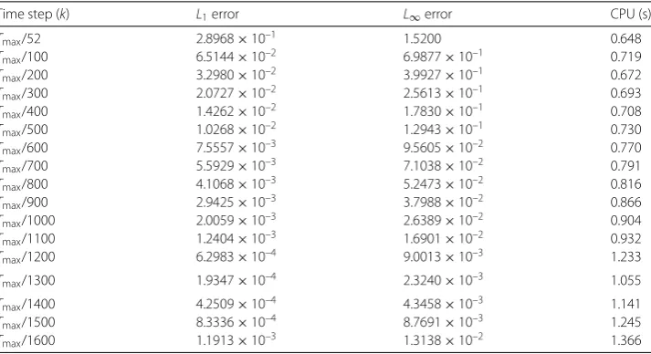
We tabulate theL1andL∞errors and display CPU times when Problems 1 and 2 are solved using FTCS at some different values of time-step size with spatial step sizeh= 0.01. The errors are displayed in Tables2and3.
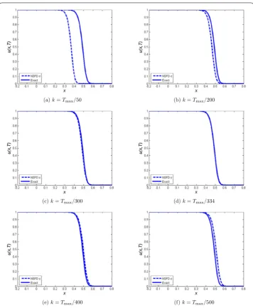
We observe from Tables2and3that theL1 andL∞ errors are almost the same with different computational times, which was expected since as we increase the length of the domain, the computational time increases. As we decrease the time-step size, theL1and L∞ errors initially decrease and reach minimum whenkTmax/1300, and then the er-rors increase again. Forkclose toTmax/50, the dispersion error is quite large. Comparing Tables2and3to Table1, we notice that theL1andL∞ errors from the FTCS method at
an optimal temporal step size are quite smaller than theL1andL∞errors from MMPDE
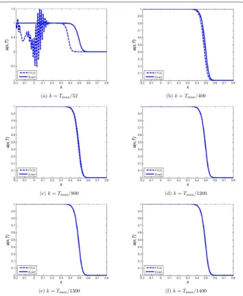
and MMDAE methods. Some plots ofuagainstxare depicted in Fig.1usingh= 0.01 and some different values ofk.
6 FTCS-
scheme
Table 2 L1andL∞errors and CPU time at some different values of time-step sizekfor Problem 1
withρ= 104at time 2.5×10⁻³with spatial mesh sizeh= 0.01 using FTCS scheme, where
Tmax= 2.5×10⁻³
Time step (k) L1error L∞error CPU (s)
Tmax/52 2.8968×10⁻¹ 1.5200 0.648
Tmax/100 6.5144×10⁻² 6.9877×10⁻¹ 0.719
Tmax/200 3.2980×10⁻² 3.9927×10⁻¹ 0.672
Tmax/300 2.0727×10⁻² 2.5613×10⁻¹ 0.693
Tmax/400 1.4262×10⁻² 1.7830×10⁻¹ 0.708
Tmax/500 1.0268×10⁻² 1.2943×10⁻¹ 0.730
Tmax/600 7.5557×10⁻³ 9.5605×10⁻² 0.770
Tmax/700 5.5929×10⁻³ 7.1038×10⁻² 0.791
Tmax/800 4.1068×10⁻³ 5.2473×10⁻² 0.816
Tmax/900 2.9425×10⁻³ 3.7988×10⁻² 0.866
Tmax/1000 2.0059×10⁻³ 2.6389×10⁻² 0.904
Tmax/1100 1.2404×10⁻³ 1.6901×10⁻² 0.932
Tmax/1200 6.2983×10⁻⁴ 9.0013×10⁻³ 1.233
Tmax/1300 1.9347×10⁻⁴ 2.3240×10⁻³ 1.055
Tmax/1400 4.2509×10⁻⁴ 4.3458×10⁻³ 1.141
Tmax/1500 8.3336×10⁻⁴ 8.7691×10⁻³ 1.245
Tmax/1600 1.1913×10⁻³ 1.3138×10⁻² 1.366
Table 3 L1andL∞errors and CPU time at some different values of time-step sizekfor Problem 2
withρ= 104at time 2.5×10⁻³with spatial mesh sizeh= 0.01 using FTCS scheme, where
Tmax= 2.5×10⁻³
Time step (k) L1error L∞error CPU (s)
Tmax/52 2.8667×10⁻¹ 1.5040 1.368
Tmax/100 6.5144×10⁻² 6.9877×10⁻¹ 2.183
Tmax/200 3.2980×10⁻² 3.9927×10⁻¹ 4.532
Tmax/300 2.0727×10⁻² 2.5613×10⁻¹ 7.689
Tmax/400 1.4262×10⁻² 1.7830×10⁻¹ 11.509
Tmax/500 1.0268×10⁻² 1.2943×10⁻¹ 16.099
Tmax/600 7.5557×10⁻³ 9.5605×10⁻² 22.270
Tmax/700 5.5929×10⁻³ 7.1038×10⁻² 28.343
Tmax/800 4.1068×10⁻³ 5.2473×10⁻² 35.383
Tmax/900 2.9425×10⁻³ 3.7988×10⁻² 43.181
Tmax/1000 2.0059×10⁻³ 2.6389×10⁻² 51.644
Tmax/1100 1.2404×10⁻³ 1.6901×10⁻² 61.532
Tmax/1200 6.2983×10⁻⁴ 9.0013×10⁻³ 71.195
Tmax/1300 1.9347×10⁻⁴ 2.3240×10⁻³ 82.456
Tmax/1400 4.2509×10⁻⁴ 4.3458×10⁻³ 94.146
Tmax/1500 8.3336×10⁻⁴ 8.7691×10⁻³ 107.725
Tmax/1600 1.1913×10⁻³ 1.3138×10⁻² 118.352
linear advection equation
ut+cux= 0, c> 0. (35)
We briefly describe their approach. To solve Eq. (35), a simple explicit consistent scheme can be constructed:
Figure 1Plot ofuagainstxfor Problem 1 using FTCS scheme at time 2.5×10⁻³at some different values ofk
andh= 0.01,Tmax= 2.5×10⁻³
The Taylor series expansion of (36) gives
1 +tDt+
t2
2! D
2 t +· · ·
uni =
(a1+a0+a–1) +x(a1–a–1)Dx
+x
2
2! (a1+a–1)D
2 x+
x3
3! (a1–a–1)D
3
x+· · ·+uni ,
whereDt=∂/∂tandDx=∂/∂x. Ruxun et al. [3] arrive at the following theorem.
Theorem 6.1 Assume that the solution u(x,t)of Eq. (35)is smooth enough and the scheme
mesh size h is small enough.Then
The Lax–Wendroff (LW) scheme discretizing Eq. (35) is given by
unm+1=1
Clearly, LW is not monotonic and is not a positive scheme. A simple approach to con-struct a monotonic scheme is to reform the LW scheme. Ruxun et al. [3] constructed the LW-scheme given by
unm+1=
Therefore LW-scheme is
unm+1=
with 0≤1. By working with dissipation and dispersion remainders, they found that
= 1/4 gives rise to a positive monotonic scheme, which still has the second-order accu-racy.
We attempt to derive the FTCS-scheme by adding numerical dissipation to the scheme to reduce numerical dispersion in the profile. We propose the following scheme:
unm+1=
The Taylor series expansion about point (n,m) gives
+3
On rearranging, we get
u– (1 +1+2+3)u+kut–h(3–1)ux–kuxx–kρu+kρu2
and the scheme is consistent.
For order of accuracy, we consider Eq. (44), replace3=1=and2= –21= –2, and
Dividing bykgives
ut–uxx–ρu+ρu2= –
The FTCS-scheme has the first-order accuracy both in time and in space.
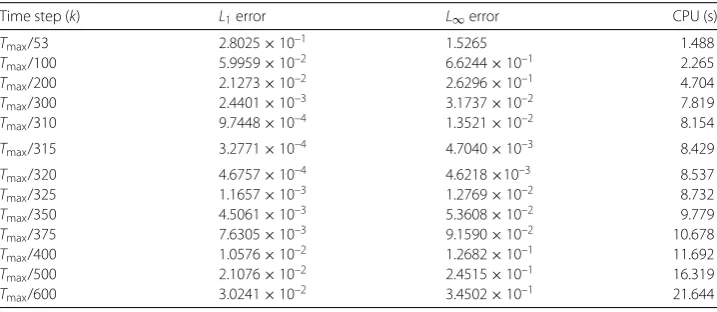
Table 4 L1andL∞errors and CPU time at some different values of time-step sizekfor Problem 1
and spatial mesh sizeh= 0.01,= 0.01 using FTCS-, whereTmax= 2.5×10⁻³
Time step (k) L1error L∞error CPU (s)
Tmax/53 2.8025×10⁻¹ 1.5265 0.764
Tmax/100 5.9959×10⁻² 6.6244×10⁻¹ 0.783
Tmax/200 2.1273×10⁻² 2.6296×10⁻¹ 0.796
Tmax/300 2.4401×10⁻³ 3.1737×10⁻² 0.928
Tmax/310 9.7448×10⁻⁴ 1.3521×10⁻² 0.850
Tmax/315 3.2771×10⁻⁴ 4.7040×10⁻³ 0.799
Tmax/320 4.6757×10⁻⁴ 4.6218×10⁻³ 0.814
Tmax/325 1.1657×10⁻³ 1.2769×10⁻² 0.902
Tmax/350 4.5061×10⁻³ 5.3608×10⁻² 0.821
Tmax/375 7.6305×10⁻³ 9.1590×10⁻² 0.927
Tmax/400 1.0576×10⁻² 1.2682×10⁻¹ 0.927
Tmax/500 2.1076×10⁻² 2.4515×10⁻¹ 0.925
Tmax/600 3.0241×10⁻² 3.4502×10⁻¹ 0.868
Table 5 L1andL∞errors and CPU time at some different values of time-step sizekand spatial mesh sizeh= 0.01,= 0.01 of Problem 2 using FTCS-, whereTmax= 2.5×10⁻³
Time step (k) L1error L∞error CPU (s)
Tmax/53 2.8025×10⁻¹ 1.5265 1.488
Tmax/100 5.9959×10⁻² 6.6244×10⁻¹ 2.265
Tmax/200 2.1273×10⁻² 2.6296×10⁻¹ 4.704
Tmax/300 2.4401×10⁻³ 3.1737×10⁻² 7.819
Tmax/310 9.7448×10⁻⁴ 1.3521×10⁻² 8.154
Tmax/315 3.2771×10⁻⁴ 4.7040×10⁻³ 8.429
Tmax/320 4.6757×10⁻⁴ 4.6218×10⁻³ 8.537
Tmax/325 1.1657×10⁻³ 1.2769×10⁻² 8.732
Tmax/350 4.5061×10⁻³ 5.3608×10⁻² 9.779
Tmax/375 7.6305×10⁻³ 9.1590×10⁻² 10.678
Tmax/400 1.0576×10⁻² 1.2682×10⁻¹ 11.692
Tmax/500 2.1076×10⁻² 2.4515×10⁻¹ 16.319
Tmax/600 3.0241×10⁻² 3.4502×10⁻¹ 21.644
For stability, we take|ξ| ≤1, which gives
2
+ k
h2
sin2
w
2
≤1 (50)
and finally yields
k h2 ≤
1
2–. (51)
Forh= 0.01 and= 0.01, we have the stability region given byk≤4.90×10⁻⁵.
We tabulate theL1andL∞errors and display CPU times for Problems 1 and 2 using FTCS-at some different values of time-step size with spatial step sizeh= 0.01 and= 0.01. The errors are displayed in Tables4and5. The time isTmax= 2.5×10⁻³, and the
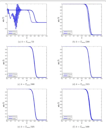
time-step size is less than or equal to 4.90×10⁻⁵. Plots ofuvsxat timeTmax= 2.5×10⁻³ are displayed in Fig.2.
Figure 2Plot ofuagainstxfor Problem 1 using FTCS-scheme at time 2.5×10⁻³and some different values
ofkandh= 0.01,= 0.01,Tmax= 2.5×10⁻³
and reach the minimum whenkTmax/315, and then the errors increase again. Fork
close toTmax/100, the dispersion error is quite large.
Comparing Tables 2and3 to Table1, we notice that theL1 andL∞ errors from the FTCS-method at an optimal step size are quite smaller than those obtained using the MMPDE and MMDAE methods.
7 Nonstandard finite difference schemes (NSFD)
sig-nificant difficulty in the computation of numerical solutions. This difficulty is numerical instabilities. Indeed, numerical instabilities are solutions to discrete equations that do not link to any solutions of the original differential equations [29]. The dynamical consistency is defined with respect to peculiar properties of a physical system, which vary mostly from one system to another. These properties must preserve positivity, boundedness, mono-tonicity of the solutions, correct number and stability of fixed-points, and other special solutions. The importance of dynamical consistency is to be taken as general standard used to restrain the possible forms for constructing an NSFD scheme [28].
7.1 Construction of NSFD schemes
The NSFD schemes are especially based upon two fundamental principles:
(1) Replacing the denominator of the discrete derivative by a more general function. (2) Nonlocal representation of both linear and nonlinear terms:
x→2xk–xk+1, (52)
x3→
xk+1+xk–1
2
x2
k, (53)
x3→2x3k–x2kxk+1, (54)
x2→
xk+1+xk+xk–1
3
xk. (55)
The selection of the functionsφ(k) for time derivatives has no general rule. Nevertheless, particular forms for precise equation can be easily found. The common functions usually used in [29] are
φ(k) =1 –e
–λk
λ , (56)
whereλis some parameter emerging in the differential equation. For partial differential equation, a suitable generalization can be made. For instance, in the nonlocalization, the nonlinear terms [29] are
u(x,t)2→ukm–1ukm+1, (57)
wherex→xm= (x)mandt→tk= (t)k. The utility and strength of NSFD procedures are that they do not need any a priori knowledge of the exact solutions to the differential equation. They come from the enforcement of certain physical system necessities on the discrete model equations as found by dynamical consistency. In conclusion, the lack of dynamical consistency leads to numerical instability. This practically appears for some values of the parameters or step-sizes [28].
Diverse explicit NSFD schemes have been suggested for Fisher’s equation with respect to their performances [18,29,30]. These performances are the stability of fixed points, positivity, boundedness of solutions, and so on. Following the idea of Mickens [31], a non-standard finite difference scheme for Eq. (6) is
un+1 m –unm
φ(t) –
un
m+1– 2unm+unm–1
[ψ(h)]2 =ρu n m–ρ
un
m+1+unm+unm–1
3
where the simple choice was made for the two denominator functions,
φ(t) =t=k; ψ(x) = (x)2=h2, (59)
and where nonlocal representation was used for theu2terms;
u2→
un
m+1+unm+unm–1
3
unm+1. (60)
A single expression of the scheme is
unm+1=(1 +kρ–
2k
h2)unm+hk2(unm+1+unm–1)
1 +kρ(u
n
m+1+unm+unm–1
3 )
. (61)
7.2 Positivity and boundedness: relation between time and space step-sizes
In this subsection, we study the positivity and boundedness properties of NSFD.
From the initial data, ifu(x, 0) =f(x) such that 0≤f(x)≤1, then we have 0≤u(x,t)≤1 [30]. If the quantityunm+1from Eq. (61) is required to satisfy the positivity condition (unm+1≥
0) ifunm≥0, then we must have
Γ = 1 +kρ– 2R≥0, R= k
h2. (62)
It follows that
1 –Γ = 2R–kρ. (63)
We have
0≤2R–kρ≤1, (64)
which gives
0≤k
2
h2–ρ ≤1. (65)
It follows that
k≤h 2
2
1 –Γ
1 –ρ2h2 and 0≤
Γ < 1, (66)
which is the condition required for positivity [30]. For stability, the amplification factorξis given by
ξ=1 +kρ–
2k
h2(1 –cos(w)) 1 +kρumax =
1 +kρ–4hk2sin2(w2)
1 +kρumax . (67)
We require|ξ| ≤1. Sinceumax= 1, we have
2k h2 sin
2
w
2
Forw∈[–π,π], we have
Note that we get the same inequality betweenhandhfor stability and positive definiteness to be satisfied. Forh= 0.01 andρ= 104, we havek≤10–4ork≤Tmax
Taking into account the symmetric condition (73), Eq. (71) can be rewritten as
unm+1= R(u
which can be rewritten
Table 6 L1andL∞errors and CPU time at some different values of time-step sizekfor Problem 1 at
time 2.5×10⁻³with spatial mesh sizeh= 0.01 using NSFD scheme, whereTmax= 2.5×10⁻³
Time step (k) L1error L∞error CPU (s)
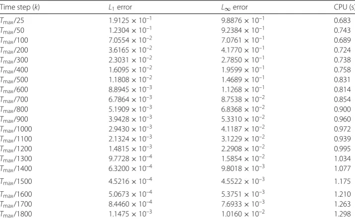
Tmax/25 1.9125×10⁻¹ 9.8876×10⁻¹ 0.683
Tmax/50 1.2304×10⁻¹ 9.2384×10⁻¹ 0.743
Tmax/100 7.0554×10⁻² 7.0761×10⁻¹ 0.689
Tmax/200 3.6165×10⁻² 4.1770×10⁻¹ 0.724
Tmax/300 2.3031×10⁻² 2.7850×10⁻¹ 0.738
Tmax/400 1.6095×10⁻² 1.9599×10⁻¹ 0.758
Tmax/500 1.1808×10⁻² 1.4689×10⁻¹ 0.831
Tmax/600 8.8945×10⁻³ 1.1268×10⁻¹ 0.814
Tmax/700 6.7864×10⁻³ 8.7538×10⁻² 0.854
Tmax/800 5.1909×10⁻³ 6.8368×10⁻² 0.900
Tmax/900 3.9428×10⁻³ 5.3310×10⁻² 0.960
Tmax/1000 2.9430×10⁻³ 4.1187×10⁻² 0.972
Tmax/1100 2.1324×10⁻³ 3.1229×10⁻² 0.939
Tmax/1200 1.4815×10⁻³ 2.2908×10⁻² 0.995
Tmax/1300 9.7728×10⁻⁴ 1.5854×10⁻² 1.034
Tmax/1400 6.3200×10⁻⁴ 9.8018×10⁻³ 1.077
Tmax/1500 4.5216×10⁻⁴ 4.5522×10⁻³ 1.175
Tmax/1600 5.0673×10⁻⁴ 5.3751×10⁻³ 1.210
Tmax/1700 8.4460×10⁻⁴ 7.6933×10⁻³ 1.263
Tmax/1800 1.1475×10⁻³ 1.0160×10⁻² 1.298
Using Eqs. (73) and (72), we have
Runm+unm+1+unm–1≤1 +kρ 3
unm+unm+1+unm–1, (79)
which gives
0≤unm+1= R(u n
m+unm+1+unm–1)
1 + (k3ρ)(un
m+1+unm+unm–1)
≤1. (80)
Hence the boundedness ofun+1 m .
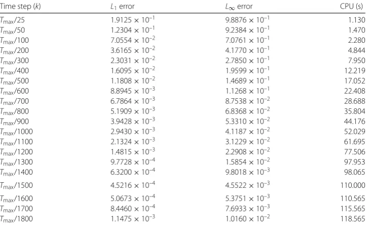
We tabulate theL1 andL∞ errors and CPU time when Problems 1 and 2 are solved using the NSFD scheme at some different values of time-step sizek, with spatial step size
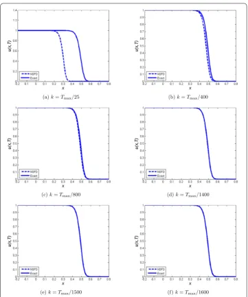
h= 0.01. The errors are displayed in Tables6and7. As the time-step size is reduced, the errors initially decrease, and optimalkis approximately equal toTmax/1500. On further decreasingk, the errors start to increase. Plots ofuvsxat some values of time-step size are displayed in Fig.3.
8 NSFD-
schemes
We construct the NSFD- by adding the expression1unm+1+2umn +3unm–1 tounm+1 to Eq. (61). We thus have
unm+1=(1 +kρ–
2k
h2)unm+hk2(unm+1+unm–1)
1 +kρ(unm+1+unm+unm–1
3 )
+1unm+1+2unm+3unm–1. (81)
Using the Taylor series expansion about (n,m), we have
u+kut+
k2
2utt+
k3
6uttt+O
Table 7 L1andL∞errors and CPU time at some different values of time-step sizekfor Problem 2 at
which can be written as
Figure 3Plot ofuagainstxfor Problem 1 using NSFD scheme at time 2.5×10⁻³at some different values ofk
andh= 0.01
+
k2
6 +
k3
6ρu+
k3
18ρh
2u xx
uttt+ρu2+
ρh2
3 uuxx
=uxx+ρu–uxx
h2
k +h
2ρu+ρh4
3 uxx
+Ok4+Oh4. (85)
We rewrite Eq. (85) in the form
ut–uxx–ρu+ρu2
= –
kρu+kρh
2
3 uxx
ut–
k
2+
k
2ρu+
k2
6ρh
2u xx
utt
–
ρh2
3 u+
h2 k +h
2ρu+ρh4
3 uxx
uxx–
k2
6 +
k3
6ρu+
k3
18ρh
2u xx
+Ok4+Oh4. (86)
We conclude that NSFD-has the first-order accuracy in time and the first-order accuracy in space.
8.1 Positivity and boundedness
We study the positivity of the method. We rewrite Eq. (81) as
unm+1=Γu
By taking the maximum ofun
j,j=m– 1,m,m+ 1, we have
m is positive if
k≤h
For stability analysis, we apply Fourier series analysis to Eq. (87) to obtain the amplifi-cation factorξ. Thus
For the stability, we have|ξ| ≤1. Sinceumax= 1, we solve
For the boundedness of NSFD-, we use the symmetric condition by takingR=Γ from Eq. (87). It follows that
which is a symmetric condition. Using Eq. (100), Eq. (87) becomes
It follows that
unm+1+unm+unm–1
3[1 –ρh32(1 – 3)]≤1 +
ρ
3
h2
3
1 – 3
1 –ρh32(1 – 3) u n
m+1+unm+unm–1
. (104)
From Eq. (99) and the symmetry condition (100) we have
Γun
m+1+unm+unm–1
≤1 +kρ 3
unm+1+unm+unm–1. (105)
It follows that
0≤unm+1= Γ(u n
m+1+unm+unm–1)
1 +k3ρ(un
m+1+unm+unm–1)
≤1. (106)
Hence the boundedness of NSFD-method. Generally without symmetry condition (100), we consider the boundedness ofun+1
m in case of NSFD, and we find the boundedness of NSFD-by stating from Eq. (81) that
0≤unm+1≤1 +unm–1– 2unm+unm+1. (107)
We rewrite(unm+1– 2unm+unm–1) as
unm–1– 2umn +unm+1=unm–1+unm+1– 2unm. (108)
Sinceunj,j=m– 1,m,m+ 1, are bounded (0≤unj ≤1), and hence from Eq. (108) we have
unm–1+unm+1– 2unm≤2– 2unm, (109)
due to the fact(unm–1+unm+1)≤2. It follows that
unm–1+unm+1– 2unm≤2– 2unm= 21 –unm. (110)
The quantity 1 –un
min Eq. (110) is bounded by
0≤1 –unm≤1. (111)
It follows from Eqs. (110) and (111) that
unm–1– 2umn +unm+1=unm–1+unm+1– 2unm≤2. (112)
Hence the boundedness ofun+1
m for NSFD-method from Eq. (107):
0≤unm+1≤1 + 2. (113)
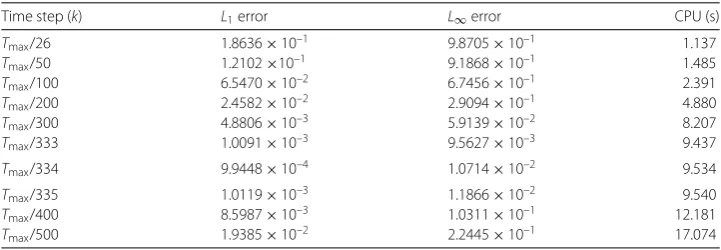
We tabulate theL1 andL∞ errors and CPU time when Problems 1 and 2 are solved
Table 8 L1andL∞errors and CPU time at some different values of time-step sizekfor Problem 1 at
time 2.5×10⁻³with spatial mesh sizeh= 0.01,= 0.01 using NSFD-scheme,Tmax= 2.5×10⁻³
Time step (k) L1error L∞error CPU (s)
Tmax/26 1.8636×10⁻¹ 9.8705×10⁻¹ 0.653
Tmax/50 1.2102×10⁻¹ 9.1868×10⁻¹ 0.662
Tmax/100 6.5470×10⁻² 6.7456×10⁻¹ 0.670
Tmax/200 2.4582×10⁻² 2.9094×10⁻¹ 0.682
Tmax/300 4.8806×10⁻³ 5.9139×10⁻² 0.699
Tmax/333 1.0091×10⁻³ 9.5627×10⁻³ 0.715
Tmax/334 9.9448×10⁻⁴ 1.0714×10⁻² 0.707
Tmax/335 1.0119×10⁻³ 1.1866×10⁻² 0.787
Tmax/400 8.5987×10⁻³ 1.0311×10⁻¹ 0.722
Tmax/500 1.9385×10⁻² 2.2445×10⁻¹ 0.780
Table 9 L1andL∞errors and CPU time at some different values of time-step size,kfor Problem 2 at
time 2.5×10⁻³with spatial mesh size,h= 0.01,= 0.01 using NSFD-scheme,Tmax= 2.5×10⁻³
Time step (k) L1error L∞error CPU (s)
Tmax/26 1.8636×10⁻¹ 9.8705×10⁻¹ 1.137
Tmax/50 1.2102×10⁻¹ 9.1868×10⁻¹ 1.485
Tmax/100 6.5470×10⁻² 6.7456×10⁻¹ 2.391
Tmax/200 2.4582×10⁻² 2.9094×10⁻¹ 4.880
Tmax/300 4.8806×10⁻³ 5.9139×10⁻² 8.207
Tmax/333 1.0091×10⁻³ 9.5627×10⁻³ 9.437
Tmax/334 9.9448×10⁻⁴ 1.0714×10⁻² 9.534
Tmax/335 1.0119×10⁻³ 1.1866×10⁻² 9.540
Tmax/400 8.5987×10⁻³ 1.0311×10⁻¹ 12.181
Tmax/500 1.9385×10⁻² 2.2445×10⁻¹ 17.074
9 Artificial viscosity
We observe from the numerical results of FTCS and NSFD that the schemes are plagued by dispersion at time step size quite close to the stability limit of the temporal step size at h= 0.01. We propose to use the artificial viscosity approach. The method of arti-ficial viscosity has been first introduced by Neumann et al. [32], who explicitly added a viscosity term to the inviscid gas dynamics equations to allow the computation of shock waves. Their approach was to change the momentum and energy equations by adding dissipation in the form of viscosity term to the pressure that would give the thickness of shock waves and also to space out the computational mesh. The artifi-cial viscosity was purposely made proportional to the second derivative uxx (which is positive in compression and negative in expansion) to ensure the mathematical consis-tency. It should satisfy some constraints: the modified equation must possess solutions without any discontinuities, the Rankine–Hugoniot conditions must hold (for conserva-tion equaconserva-tions), and the dissipative term must be negligible outside of the shock waves [33].
Figure 4Plot ofuagainstxfor Problem 1 using NSFD-scheme at time 2.5×10⁻³at some different values ofkandh= 0.01,= 0.01
Finally, it has been specified by Caramana et al. [38] that an artificial viscosity should have the following properties:
1. Dissipativity: The artificial viscosity must only act to decrease the kinetic energy. 2. Galilean invariance: The viscosity should vanish smoothly as the velocity field
becomes constant.
3. Self-similar motion invariance: The viscosity should vanish for uniform contraction and rigid rotation.
4. Wave-front invariance: The viscosity should have no effect along a wave front of constant phase on a grid aligned with shocks.
We start with a simple linear advection equation,ut+ux= 0 (Eq. (35) withc= 1). We add the artificial viscosityσhuxxto obtain
ut+ux=σhuxx. (114)
As h→0, we recover the initial linear advection equation ut+ux= 0, and σ is a real parameter. The numerical discretization for Eq. (114) is
un+1
2x are respectively forward, backward, and centered differencing operators. Rewriting Eq. (115), we have
unm+1=unm–kD0unm+σkhD+D–unm. (116)
Ash→0, the scheme given by Eq. (116) is a consistent approximation of Eq. (35) with
c= 1.
9.1 FTCS with artificial viscosity
We need to solve
ut=uxx+ρu(1 –u). (117)
We addσhuxxand obtain the new equation
ut=uxx+ρu(1 –u) +σhuxx. (118)
The numerical scheme used to discretize Eq. (118) is
un+1
which can be rewritten as
unm+1=
For the order of accuracy, the Taylor series expansion about the point (n,m) of (120) gives
Table 10 L1andL∞errors CPU time at some different values of time-step sizekfor Problem 1 with
ρ= 104at time 2.5×10⁻³with spatial mesh sizeσ= 2.0 andh= 0.01 using FTCS with artificial viscosity
Time step (k) L1error L∞error CPU (s)
Tmax/53 2.6947×10⁻¹ 1.5155 0.737
Tmax/100 6.2546×10⁻² 6.8175×10⁻¹ 0.737
Tmax/200 3.0034×10⁻² 3.6771×10⁻¹ 0.742
Tmax/300 1.7645×10⁻² 2.1809×10⁻¹ 0.758
Tmax/400 1.1108×10⁻² 1.3983×10⁻¹ 0.782
Tmax/500 7.0695×10⁻³ 8.9529×10⁻² 0.800
Tmax/600 4.3263×10⁻³ 5.5222×10⁻² 0.847
Tmax/700 2.3414×10⁻³ 3.0552×10⁻² 0.856
Tmax/800 8.5592×10⁻⁴ 1.2040×10⁻² 0.907
Tmax/850 3.1048×10⁻⁴ 4.4291×10⁻³ 0.913
Tmax/860 2.2700×10⁻⁴ 3.0141×10⁻³ 0.918
Tmax/870 1.6308×10⁻⁴ 1.8608×10⁻³ 0.923
Tmax/880 1.3833×10⁻⁴ 2.3032×10⁻³ 0.926
Tmax/890 2.3267×10⁻⁴ 2.9465×10⁻³ 0.930
Tmax/900 3.3881×10⁻⁴ 3.6042×10⁻³ 0.951
Tmax/1000 1.2861×10⁻³ 1.4273×10⁻² 0.967
Tmax/1100 2.0648×10⁻³ 2.3789×10⁻² 1.001
Tmax/1200 2.7162×10⁻³ 3.1756×10⁻² 1.042
Tmax/1300 3.2692×10⁻³ 3.8522×10⁻² 1.071
Tmax/1400 3.7445×10⁻³ 4.4336×10⁻² 1.124
Tmax/1500 4.1573×10⁻³ 4.9385×10⁻³ 1.142
which gives
ut–uxx–ρu(1 –u) = –
k
2utt–
k2
6uttt+σhuxx+O
k3+O
h4
k
. (122)
We conclude that FTCS with artificial viscosity has the first-order accuracy in time and the first-order accuracy in space.
If σ = 0, then we recover the FTCS scheme. The amplification factorξ of the FTCS scheme with artificial viscosity is
ξ= 1 +2k
h2(1 +σh)
cos(w) – 1+kρ1 –|umax|. (123)
We chooseumax= 1 based on the numerical experiment chosen and have
ξ= 1 –4k
h2(1 +σh)sin 2
w
2
. (124)
The stability region is
k<h
2
2
1
1 +σh . (125)
We chooseσ= 2.0 andh= 0.01 and obtaink< 4.9020×10⁻⁵orTmax/51.
We tabulate theL1andL∞errors and CPU time when Problem 1 is solved using FTCS
with artificial viscosity at some different values of time-step sizekwith spatial step size
Figure 5Plot ofuagainstxfor Problem 1 using FTCS with artificial viscosity at time 2.5×10⁻³at some
different values ofkandh= 0.01,σ= 2.0,Tmax= 2.5×10⁻³
9.2 Nonstandard finite difference method with artificial viscosity
The nonstandard finite difference scheme with artificial viscosity to discretize Eq. (118) is
unm+1–unm
k =
unm+1– 2unm+unm–1
h2 +ρu
n m–ρ
unm+1+unm+unm–1
3
unm+1
+σh
un
m+1– 2unm+unm–1 h2
. (126)
A single expression for the scheme is
unm+1=(1 +kρ– 2β)u n
m+β(unm+1+unm–1)
1 +kρ(unm+1+unm+unm–1
3 )
, whereβ= k
The Taylor series expansion of this scheme about (m,n) gives
which can be written as
ut–uxx–ρu+ρu2–σhuxx
We conclude that NSFD with artificial viscosity has the first-order accuracy in time and the first-order accuracy in space.
9.2.1 Positivity and boundedness
The scheme given by Eq. (127) is positive ifΓ = 1 +kρ–2k
h2(1 +σh)≥0. Hence the scheme is positive definite under the conditions
k≤h
For boundedness, we start by assuming that 0≤un
m≤1. We apply the same steps as in case of NSFD without artificial viscosity by letting
Γ = 1 +kρ– 2R, R=β= k
h2(1 +σh), (131)
and we use the symmetric condition
R= k
Hence the boundedness ofun+1 m .
We tabulate theL1andL∞errors, CPU time when Problem 1 is solved using NSFD with
artificial viscosity scheme at some different values of time-step sizekwith spatial step size
Figure 6Plot ofuagainstxfor Problem 1 using NSFD with artificial viscosity at time 2.5×10⁻³, at some different values ofkandh= 0.01,σ= 2.0,Tmax= 2.5×10⁻³
10 Conclusion
In this work, we have initially used the FTCS and NSFD schemes to solve Fisher’s equation when the coefficient of diffusion is much less than the coefficient of reaction term and the initial condition consists of an exponential function. The time-step size must be relatively small to obtain accurate results, and the CPU time becomes large if the domain is large.
We propose four schemes, namely FTCS-, NSFD-, FTCS with Artificial Viscosity, and NSFD with artificial viscosity, which give quite accurate results at larger time-step size and, consequently, a smaller CPU time as compared to the FTCS and NSFD methods. Also, the
Table 11 L1andL∞errors and CPU time at some different values of time step sizekfor Problem 1 at
time 2.5×10⁻³with spatial mesh sizeh= 0.01,σ= 2.0 using NSFD with artificial viscosity method
Time step (k) L1error L∞error CPU (s)
Tmax/25 1.8982×10⁻¹ 9.8811×10⁻¹ 0.891
Tmax/50 1.2102×10⁻¹ 9.1869×10⁻¹ 0.893
Tmax/100 6.8010×10⁻² 6.9128×10⁻¹ 0.897
Tmax/200 3.3252×10⁻² 3.8653×10⁻¹ 0.928
Tmax/300 1.9973×10⁻² 2.4143×10⁻¹ 0.998
Tmax/400 1.2961×10⁻² 1.5892×10⁻¹ 0.999
Tmax/500 8.6255×10⁻³ 1.0838×10⁻¹ 1.019
Tmax/600 5.6799×10⁻³ 7.3290×10⁻² 1.041
Tmax/700 3.5494×10⁻³ 4.7746×10⁻² 1.089
Tmax/800 1.9544×10⁻³ 2.8406×10⁻² 1.355
Tmax/900 8.4110×10⁻⁴ 1.3294×10⁻² 1.355
Tmax/950 5.2648×10⁻⁴ 7.1035×10⁻³ 1.564
Tmax/1000 4.4308×10⁻⁴ 5.5908×10⁻³ 1.664
Tmax/1050 7.8758×10⁻⁴ 8.5810×10⁻³ 1.683
Tmax/1100 1.1865×10⁻³ 1.1836×10⁻² 1.684
Tmax/1200 1.8866×10⁻³ 1.9106×10⁻² 1.687
Tmax/1300 2.4809×10⁻³ 2.5706×10⁻² 1.688
Tmax/1400 2.9918×10⁻³ 3.1732×10⁻² 1.690
Tmax/1500 3.4356×10⁻³ 3.6977×10⁻² 1.745
Acknowledgements
The authors are grateful to the anonymous reviewers for their very constructive comments and suggestions, which have helped to improve the paper considerably.
Funding
A.R. Appadu and K.M. Agbavon are grateful to the South African DST/NRF SARChI on Mathematical Models and Methods in Bioengineering and Biosciences (M3B2), Grant 82770 for funding.
Competing interests
None of the three authors has competing interests in the manuscript.
Consent for publication
The authors agree for the paper to be published.
Authors’ contributions
Each of the authors contributed to the work and read and approved the final version of the manuscript.
Author details
1Department of Mathematics and Applied Mathematics, University of Pretoria, Pretoria, South Africa.2Department of Mathematics, University of South Africa, Florida, South Africa.
Publisher’s Note
Springer Nature remains neutral with regard to jurisdictional claims in published maps and institutional affiliations.
Received: 8 November 2018 Accepted: 3 April 2019 References
1. Li, S., Petzold, L., Ren, Y.: Stability of moving mesh systems of partial differential equations. SIAM J. Sci. Comput.20, 719–738 (1998)
2. Qiu, Y., Sloan, D.M.: Numerical solution of Fisher’s equation using a moving mesh method. J. Comput. Phys.146, 726–746 (1998)
3. Ruxun, L., Mengping, Z., Ji, W., Xiao-Yuan, L.: The designing approach of difference schemes by controlling the remainder-effect. Int. J. Numer. Methods Fluids31, 523–533 (1999)
4. Zeidan, D., Romenski, E., Slaouti, A., Toro, E.F.: Numerical study of wave propagation in compressible two-phase flow. Int. J. Numer. Methods Fluids54, 393–417 (2007)
5. Zeidan, D.: Assessment of mixture two-phase flow equations for volcanic flows using Godunov-type methods. Appl. Math. Comput.272, 707–719 (2016)
6. Goncalves da Silva, E., Zeidan, D.: Numerical simulation of unsteady cavitation in liquid hydrogen flows. Int. J. Eng. Syst. Model. Simul.9, 41 (2017)
7. Minhajul, Zeidan, D., Raja Sekhar, T.: On the wave interactions in the drift-flux equations of two-phase flows. Appl. Math. Comput.327, 117–131 (2018)
9. Yatat, V., Couteron, P., Dumont, Y.: Spatially explicit modelling of tree-grass interactions in fire-prone savannas (a partial differential equations framework). Ecol. Complex..36, 290–313 (2018)
10. Doelman, A., Kaper, T.J., Zegeling, P.A.: Pattern formation in the one-dimensional Gray–Scott model. Nonlinearity10, 523–563 (1997)
11. Houdek, G., Balmforth, N.J., Christensen-Dalsgaard, J., Gough, D.O.: Amplitudes of stochastically excited oscillations in main-sequence stars (1999). ArXiv PreprintAstro-ph/9909107
12. Hagberg, A., Meron, E.: From labyrinthine patterns to spiral turbulence. Phys. Rev. Lett.72, (1994) 13. Fisher, R.A.: The wave of advance of advantageous genes. Ann. Hum. Genet.7, 355–369 (1937)
14. Kolmogorov, A.N., Petrovsky, I.G., Piskunov, N.S.: Etude de l’équation de la diffusion avec croissance de la quantité de matiere et son application à un problème biologique. J. Mosc. Univ. Math. Bull.129, 1–25 (1937)
15. Hagstrom, T., Keller, H.B.: The numerical calculation of traveling wave solutions of nonlinear parabolic equations. SIAM J. Sci. Stat. Comput.7, 978–988 (1986)
16. Gazdag, J., Canosa, J.: Numerical solution of Fisher’s equation. J. Appl. Probab.11, 445–457 (1974)
17. Canosa, J.: On a nonlinear diffusion equation describing population growth. IBM J. Res. Dev.17, 307–313 (1973) 18. Anguelov, R., Kama, P., Lubuma, J.M.S.: On non-standard finite difference models of reaction–diffusion equations.
J. Comput. Appl. Math.175, 11–29 (2005)
19. Mulholland, L.S., Qiu, Y., Sloan, D.M.: Solution of evolutionary partial differential equations using adaptive finite differences with pseudospectral post-processing. J. Comput. Phys.131, 280–298 (1997)
20. Huang, W., Ren, Y., Russell, R.D.: Moving mesh partial differential equations (MMPDES) based on the equidistribution principle. SIAM J. Numer. Anal.31, 709–730 (1994)
21. Huang, W., Ren, Y., Russell, R.D.: Moving mesh methods based on moving mesh partial differential equations. J. Comput. Phys.113, 279–290 (1994)
22. Chen-Charpentier, B.M., Kojouharov, H.V.: An unconditionally positivity preserving scheme for advection–diffusion reaction equations. Math. Comput. Model.57, 2177–2185 (2013)
23. Durran, D.R.: Numerical Methods for Fluid Dynamics with Applications to Geophysics, vol. 32. Springer, Berlin (2010) 24. Taha, T.R., Ablowitz, M.I.: Analytical and numerical aspects of certain nonlinear evolution equations, III. Numerical,
Korteweg–de Vries equation. J. Comput. Phys.55, 231–253 (1984)
25. Zabusky, N.J., Kruskal, M.D.: Interaction of solitons in a collisionless plasma and the recurrence of initial states. Phys. Rev. Lett.15, 240 (1965)
26. Appadu, A.R., Lubuma, J.M.S., Mphephu, N.: Computational study of three numerical methods for some linear and nonlinear advection–diffusion–reactions problems. Prog. Comput. Fluid Dyn.17, 114–129 (2017)
27. Mickens, R.E.: Exact solutions to a finite-difference model of a nonlinear reaction–advection equation: implications for numerical analysis. Numer. Methods Partial Differ. Equ.5, 313–325 (1989)
28. Mickens, R.E.: Dynamic consistency: a fundamental principle for constructing nonstandard finite difference schemes for differential equations. J. Differ. Equ. Appl.11, 645–653 (2005)
29. Mickens, R.E.: Nonstandard finite difference models of differential equations (1994)
30. Mickens, R.E.: Relation between the time and space step-sizes in nonstandard finite-difference schemes for the Fisher equation. Numer. Methods Partial Differ. Equ.13, 51–55 (1997)
31. Mickens, R.E.: Nonstandard finite difference schemes for differential equations. J. Differ. Equ. Appl.8, 823–847 (2002) 32. VonNeumann, J., Richtmyer, R.D.: A method for the numerical calculation of hydrodynamic shocks. J. Appl. Phys.21,
232–237 (1950)
33. Campbell, J.C., Shashkov, M.J.: A tensor artificial viscosity using a mimetic finite difference algorithm. J. Comput. Phys.
172, 739–765 (2001)
34. Noh, W.F., Protter, M.H.: Difference methods and the equations of hydrodynamics. J. Math. Mech.12, 149–191 (1963) 35. Landshoff, R.: A numerical method for treating fluid flow in the presence of shocks (1955)
36. Wilkins, M.L.: Use of artificial viscosity in multidimensional fluid dynamic calculations. J. Comput. Phys.36, 281–303 (1980)
37. Kurapatenko, V.F.: Difference methods for solutions of problems of mathematical physics. Am. Math. Soc. (1967) 38. Caramana, E.J., Shashkov, M.J., Whalen, P.P.: Formulations of artificial viscosity for multi-dimensional shock wave