Volume 2010, Article ID 716565,11pages doi:10.1155/2010/716565
Research Article
Characterizing the Path Coverage of
Random Wireless Sensor Networks
Moslem Noori, Sahar Movaghati, and Masoud Ardakani
Department of Electrical and Computer Engineering, University of Alberta, Edmonton, Canada T6G 2V4
Correspondence should be addressed to Moslem Noori,[email protected]
Received 1 November 2009; Accepted 24 February 2010
Academic Editor: Xinbing Wang
Copyright © 2010 Moslem Noori et al. This is an open access article distributed under the Creative Commons Attribution License, which permits unrestricted use, distribution, and reproduction in any medium, provided the original work is properly cited.
Wireless sensor networks are widely used in security monitoring applications to sense and report specific activities in a field. In path coverage, for example, the network is in charge of monitoring a path and discovering any intruder trying to cross it. In this paper, we investigate the path coverage properties of a randomly deployed wireless sensor network when the number of sensors and also the length of the path are finite. As a consequence, Boolean model, which has been widely used previously, is not applicable. Using results from geometric probability, we determine the probability of full path coverage, distribution of the number of uncovered gaps over the path, and the probability of having no uncovered gaps larger than a specific size. We also find the cumulative distribution function (cdf) of the covered part of the path. Based on our results on the probability of full path coverage, we derive a tight upper bound for the number of nodes guaranteeing the full path coverage with a desired reliability. Through computer simulations, it is verified that for networks with nonasymptotic size, our analysis is accurate where the Boolean model can be inaccurate.
1. Introduction
Wireless sensor networks (WSNs) have many applications in security monitoring. In such applications, since it is essential to keep track of all activities within the field, network coverage is of great importance and must be considered in the network design stage.
Path coverage is one of the monitoring examples, where WSNs are deployed to sense a specific path and report
possible efforts made by intruders to cross it. In a manual
network deployment, the desired level of the path coverage can be achieved by proper placement of the sensors over the area. When it is not possible to deploy the network manually, random deployment, for example, dropping sensors from an aircraft, is used. Due to the randomness of the sensors location, network coverage expresses a stochastic behavior and the desired (full) path coverage is not guaranteed. Thus, a detailed analysis of the random network coverage can be ultimately useful in the network design stage to determine the node density for achieving the desired area/path cover-age.
Path coverage by a random network (or barrier coverage which is a relaxed version of the path coverage) has been the focus of some previous work [1–6]. In [1], assuming that a random network is deployed over an infinite area with nodes following a Poisson distribution, authors investigate the path coverage of the network. They first study the path coverage over an infinite straight line when the sensor has a random sensing range. Then, they show that in the asymptotic situation, where the sensing range of the sensors tends to 0 and the node density approaches infinity, the results are extendible to finite linear and curvilinear paths. Further, a path coverage analysis is proposed for a high-density Poisson-distributed network in [2] where sensors have a fixed sensing range. The path coverage analysis of
[1,2] is based on the Boolean model of [7], where a Poisson
point process is justified.
Kumar et al. study k-barrier coverage provided by a
propose an algorithm determining whether an area is k -barrier covered or not. Also, they introduce the concepts of weak and strong barrier coverage over the belt and derive the condition on the sensors density guaranteeing the weak barrier coverage.
The focus of [4] is on the strong barrier coverage. First, authors present a condition insuring the strong barrier coverage over a strip where the sensors locations follow a Poisson point process. Then, by considering asymptotic situation (on the network size and number of nodes) and using Percolation theory [8], they determine, with a probability approaching 1, whether the network has a strong barrier coverage or not. Then, they use their analysis to devise a distributed algorithm to build strong barrier coverage over the strip.
In this work, unlike most existing studies which focus on asymptotic setups, we study the path coverage of a finite random network (in terms of both network size and the number of nodes). As a result, the Boolean model is not accurate. Alternatively, the methodology of this work is based on some results from geometric probability. Our focus is on the path coverage for a circle, but extension to other path shapes is briefly discussed.
In the ideal case, all sensors are located exactly on the path. This, however, is not a practical assumption for randomly deployed networks. To consider the inaccuracy of the sensors locations, we assume that sensors are inside a ring containing the circular path. As a result, the portion of the path covered by any given sensor is not deterministic.
Moreover, other factors may affect the sensing range of a
sensor. Thus, our analysis is not based on a fixed sensing range. Indeed, we first develop a random model for the covered segment of the path by each sensor. Then, we study the distribution of the number of uncovered gaps on the path. The full path coverage is a special case where the number of gaps is zero. This is used to determine a tight bound on the number of active sensors assuring the full path coverage with a desired reliability. Also, we find the probability of having all possible gaps smaller than a given size. This probability reflects the reliability of detecting an intruding object with a known size.
In addition to studying the number of gaps, we present a simplified analysis for deriving the cumulative distribution function (cdf) of the covered part of the path. This simplified analysis is based on using the expected value of the covered part of the path by a sensor instead of considering the precise random model. We observe that the simplified analysis can provide a fairly accurate approximation of the path coverage.
Since our analysis studies the effect of the number of
nodes on the path coverage of a finite size network, it can readily be used in the design of practical networks. In fact, using our results, one can determine the number of nodes in the network to satisfy a desired level of coverage. An example is provided.
The paper is organized as follows.Section 2introduces
the network model and defines the problem. Our coverage
analysis is presented in Section 3.Section 4 includes
com-puter simulations verifying our analysis. Finally, Section 5
concludes the paper.
P
w w
r
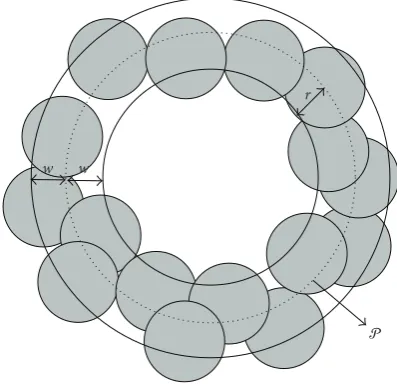
Figure1: Network structure.
2. Preliminary
2.1. Network Model. We consider N sensors monitoring a
circular path with unit circumference, calledP. In an ideal
case, the sensors are precisely located on the circular path, but this is not usually true for a randomly deployed network. In order to take this fact into account, we assume that
sensors are randomly spread over a ring containingP (See
Figure 1). We assume a symmetric distribution for sensors, that is, the sensor density does not depend on the polar angle and is determined only by the distance from the center. It is generally desired to have more sensors in the vicinity
ofP.Thus, distributions with larger values close toP are
preferred. When no effort is made to put the sensor as close as
possible to the path (Nsensors are spread totally randomly),
the uniform distribution is obtained. Hence, in the sense
of placement efforts, uniform distribution reflects the worst
case. We consider uniform distribution to verify our analysis
by computer simulation inSection 4. Our analysis, however,
is presented for any given symmetric distribution. Also, notice that since the number of sensors is finite and known, Poisson distribution, which has been the focus of existing asymptotic analysis, is not applicable.
We also assume that sensors sensing range may vary from
r1tor2. Obviously, for a fixed sensing range, modelr1=r2.
Without loss of generality, it is assumed that the width of the
ring is smaller than or equal to 2r2and the desired circular
path is located at the middle of the ring. Since the sensors
farther than r2 to the path do not contribute to the path
coverage, our assumption on the ring width does not hurt the generality of the analysis.
(i)Distribution of the number of gaps. Due to the randomness of the network implementation, sensors may not cover the whole path. In this case, one
or more gaps appear. Assume that g represents the
number of gaps onP. We are interested to find the
probability of havingmgaps, shown byP(g=m).
(ii)Full path coverage.It is desired to provide a complete coverage of the path. Since the full path coverage is identical to having no gaps, one can equivalently find
P(g =0). This can simply be found from the derived
distribution ofg.
(iii)Reliability of the network in detecting objects. It is
important to investigate whether the network is able to detect an object, while the path is not fully covered and there may exist some gaps. Basically, we need to consider the size of the gaps in addition to their number. If one knows the size of the intruders beforehand, it is not necessary to provide the full path coverage. Instead, it is possible to deploy a network such that while the path is not fully covered, the size of the possible gaps is smaller than the intruders. Clearly, implementing a network with possible small gaps requires fewer number of nodes and consequently is less expensive. To this end, we find the probability of having all gaps smaller than
a given lengtht, denoted byP(lg < t).
(iv)Distribution of the covered part of the path. The
covered part of the path,C, has a stochastic nature
and its distribution provides a general view of the entire path coverage. In fact, the covered part of the
network reflects the combined effect of the number
of gaps and their sizes. We derive the cdf ofC,FC(x).
3. Path Coverage Analysis
In this section, we present our analysis of the path coverage. For this purpose, we take advantage of existing results in geometric probability and extend them to our case. After the exact coverage analysis, a less complex approximate analysis is also presented.
An arbitrary point on P is covered if it is within the
sensing range of at least one sensor. Here, we assume
that the sensing area of sensor i is a circle denoted by
si,i=1, 2,. . .,N. The covered part of the path by eachsiis
its intersection withP which is an arc, calledai. Thus, the
total covered part of the path is
C= N
i=1
ai. (1)
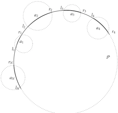
Notice that the length of ai’s depends on the location of
the sensor within the ring-shaped network area and its sensing range. Considering an arbitrary point as the origin
onP and choosing the clockwise direction as the positive
direction, each ai starts from li and continues (clockwise)
untilri, (Figure 2). In other words, li determines the most
left point of the arc andrispecifies the most right point of
the arc. There are two noteworthy issues here. First, the size
lN
Figure2: The random arcs placed clockwise onP.
ofai’s and their positions are random because of the random
placement of the sensors over the ring. Second, C is not
necessarily connected and there may exist several uncovered
gaps onP. The number of uncovered gaps onP and their
size can reflect the possible opportunities for intruders to
passP without being detected by the sensors. Ifg =0,P is
fully covered.
The problem of covering a circle with random arcs has been studied in geometric probability [9–15]. In some cases,
it is assumed that the arcs have a fixed length [9,12,13,15] or
the analysis is conducted in the asymptotic situation [10,14].
Asymptotic analysis is suitable for the situation where the
sizes ofsi’s are significantly smaller thanP. In the following,
we initially use the result of [11] on the coverage of a circle with random arcs of random sizes. This helps us to provide an exact explanation of the path coverage. Then, we use
the mean value ofai’s to provide a simplified approximate
analysis based on the fixed-length random arc placement over the circle [12].
3.1. Exact Analysis. We apply the following theorem from [11] to find the exact distribution of the number of gaps on
P.
Theorem 1. Assume thatNarcs are distributed independently
with a uniform distribution over a circle of circumference 1. If
F(·)shows the cdf of the arc length over[0, 1], the distribution of the number of uncovered gaps on the circle,g, is
Pg=m=
To applyTheorem 1for finding the number of uncovered
gaps on P, we first prove the uniformity of the arc
distribution overP in the following lemma.
Lemma 1. For a symmetric distribution of the sensors over the
path, the location of the intersection of the sensors sensing range andP is uniformly distributed overP.
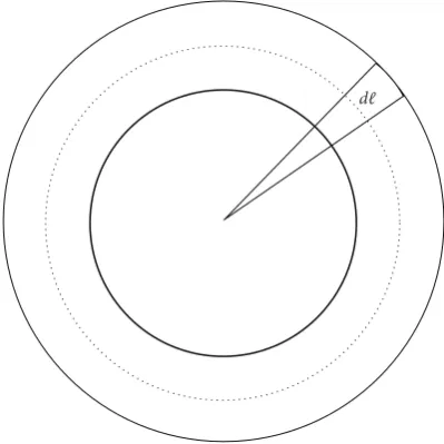
Proof. We equivalently show that the center points of the arcs are uniformly distributed over the circle. For this purpose,
consider a small element with length d → 0 on P.
Then, we build a sector of the ring based on this length element whose left and right sides pass the left and right ends of the length element (Figure 3). The center point of the arcs, resulted from the intersection of the sensing area
of the nodes within the sector andP, falls withind. Due
to the independence of the sensors distribution from the
polar angle, all elements with length d on the circle have
the same chance to include an arc center point. Therefore, the distribution of the arc centers, and consequently arc
locations, is uniform onP.
FollowingLemma 1, in order to find the distribution of
the number of gaps onP, we needF(·) or in our caseFa(·),
the cdf ofai’s. Notice thatai’s are independent and identically
distributed (i.i.d) random variables. We find Fa(·) in the
appendix for arbitrary distributions of sensor location and sensing range.
As a result of Theorem 1 and Lemma 1, we have the
following corollary.
Corollary 1. The probability of the full path coverage,Pf, is
Pf =P
Furthermore, one can show that the expected number of gaps onP is [11]
Eg=N1−μaN−1, (5)
whereμais the mean ofai’s.
E(g) can be used to find an upper bound on the number
of nodes in the network guaranteeing the full path coverage with a given reliability. This is presented below.
Corollary 2. To guarantee a full path coverage with
probabil-ityp, the following relation holds
N1−μaN−1≥1−p. (6)
Proof. Recall Markov’s inequality for a positive random
variableX
P(X≥b)≤E(X)
b , (7)
d
Figure3: Distribution of the arc position over the circle.
whereb >0. If we letXbe the random variable of the number
of gapsg, and putb=1, we have
Pg≥1≤Eg. (8)
Combining (5) and (8) results in (6).
Using (6), it is straightforward to find an upper bound
onN guaranteeing a desired level of coverage, p. Later, our
simulations show that this bound is in fact very tight. Another feature of the path coverage that we like to study is the quality of the coverage in terms of the size of the gaps
onP. Assume that we like to guarantee detecting any object
bigger than a particular size, sayt. To assure detecting such
objects, all of the gaps have to be smaller thant. Hence, we
like to find the probability of having no gaps larger than t,P(lg < t), wherelg is the length of the largest gap onP.
Corollary 3. The probability of having no gaps larger thantis
Plg< t=
Proof. Consider a realization of the random placement of arcs on the path. Now, one can consider a scenario where
the length of each arc is increased byt. If there exists a gap
smaller thantin the first scenario, this gap will be covered
in the second scenario since the arcs are t longer. On the
other hand, a gap with any size in the second scenario will
that the above discussion is valid for any realization of the network. Thus, instead of investigating the probability of
having no gaps longer thantin the first scenario, we look
for the probability of the full coverage in the second scenario.
Denoting the length of the arcs in the second scenario byai,
one can think of them as being drawn from the distribution
fa(x)= fa(x−t) or equivalently
Fa(x)=Fa(x−t). (10)
This completes the proof.
Using the same approach taken for finding the upper
bound onNin (6), one can derive an upper bound on the
number of nodes to guarantee having all gaps smaller thant.
We also like to investigateC, that is, the portion ofP
which is covered by the nodes. To find C, we first reorder
the arcs based on their starting points,li’s. Thusl1 < l2 <
l3 <· · · < lN. Now, we divideP to arcsbi, wherebi is an
arc starting fromliand ending atli+1. Finally,bN starts from
lN and ends atl1. Since we haveNrandom arcs intersecting
withP, there existNof such spacings on the circle. TheseN
spacings may or may not be covered by the network. Adding the covered parts of the path together, we have
C=
Notice that in (12) we assume rotational indices forai−j’s.
It means that ifi−j <1 we replace the index withN−i+j. In
(12),xiis the length of the connected part ofCstarting from
liand continuing clockwise. Whenyi≤xi, the whole spacing
yiis covered and min(·,·) function should returnyi. When
xi< yi, a portion ofyiremains uncovered and there exists a
gap at the right side ofyi. Thus, min(·,·) function returnsxi.
It is noteworthy that because of the problem symmetry,zi’s
are identically distributed random variables. Thus, we use a
single random variablezto refer to them.
The distribution of C can be well approximated by a
Gaussian distribution using central limit theorem (CLT)
where the mean value of C, μC, is μC = Nμz. Here, μz
denotes the mean value ofz. Also,σ2
C =Nσz2whereσC2 and
σ2
z represent the variance ofCandz, respectively. In reality,
one can safely simplify (12) to
xi=maxai,ai−1−yi−1. (13)
This is becauseai’s are i.i.d. and thus it is very unlikely that,
for example,ai−2−yi−1−yi−2> ai.
3.2. Approximate Analysis. In the following, we present an approximate analysis simplifying our path coverage study. The idea of this approximate analysis is to consider a model
where a set of fixed-length arcs are spread randomly overP
instead of using the actual random-sized arcs. The length of these fixed arcs is equal to the mean value of the random-sized arcs in the original case. We denote the mean value of
these random arcs withμa. In this case, it can be shown that
the number of uncovered gaps onP is distributed as follows
[12]:
applicable to find the probability of having no gaps larger
than tonP. For this purpose, we just need to use μa +t
instead ofμa in (14). In addition, the distribution ofCcan
be derived when the arc size is fixed [12]. In this case, we have
FC(x)=
this aim, we first consider the uncovered part of the path,V,
and find its expected value, calledμV. ThenμCcan be found
using the factμC=1−μV.
An arbitrary pointxonPremains uncovered when there
is noaicovering it. This is equivalent to having none ofli’s
within an arc with lengthμawhose right end point isx. There
areNsensors in the network, hence, the probability of having
xuncovered,μV, is
3.3. Some Remarks
Remark 1. Our path coverage analysis is applicable to any closed path, for example, ellipse, with finite length when the location of the path segment covered by an arbitrary sensor is uniformly distributed over the path. For this purpose, we just need to have the distribution of the intersection of sensors sensing range and the path. Also, the analysis is applicable to linear path coverage. In fact, the problem of covering a circle with random arcs can be transformed to the problem of
covering a piece of line, say the interval [0,b], with random
Remark 2. In many WSNs, the number of active sensors in the network changes with time. This can be due to, for example, sleep scheduling or death of some nodes. Since our
analysis is provided for arbitrary N, it can accommodate
such situations, simply by replacingNwithN(t) in relevant
equations. Consequently, the coverage can be studied as a function of time.
4. Simulation
In this section, we demonstrate the accuracy of our analysis via computer simulations. We have inspected two scenarios for the sensors sensing range. In the first scenario, we assume
a network with N sensors all having a fixed sensing range
equal tor. The sensors are uniformly deployed inside a ring
around the circular path, whereP has unit circumference.
In the second scenario, the sensors sensing range is also
uniformly distributed between 0 and rmax. A zero sensing
range can represent a dead sensor.
We evaluate random properties such as the full coverage, number of uncovered gaps, tightness of the bound presented in (6), the intruder detectability, and the portion of the covered path using simulation, and compare the results with our theoretical analysis.
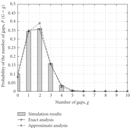
4.1. Uncovered Gaps. Probability density of the number of
uncovered gaps on the path, P(g = m), was derived in
Section 3.1. Figure 4 shows the probability mass function
(pmf) of the number of uncovered gaps via simulation
for N = 30. Here, we have assumed that the sensing
range of all sensor nodes is fixed and is equal to 0.06.
The theoretical results using (2) have also been sketched for comparison. It can be concluded that the formulation
derived inSection 3.1quite accurately describes the pmf of
the number of uncovered gaps on the path. The third curve in Figure 4is the result of approximation analysis inSection 3.2.
Parameterμain (14) is set to be the expected value of random
variablea, derived in the appendix.
It is clear from Figure 4 that the results from the
approximate analysis are fairly close to the exact analysis and the simulations. Due to the complexity of the evaluation of exact analysis, we compare the rest of our simulation results
with the approximate analysis presented in Section 3.2 to
characterize the coverage properties of the network.
In the case of fixed sensing range, as the width of the
ring becomes smaller, the variance ofadecreases and the arc
lengths become closer toμa, making the approximate analysis
more accurate. To study the worst case, in our analysis, we
assume the ring widthwis equal to 2r. Notice that any node
outside this ring does not contribute to the path coverage.
For random sensing range, we choosew = rmax/2. Notice
that sincer1=0, there will be nodes in the ring that will not
contribute to the path coverage.
Figures 5 and 6 demonstrate the probability of full
coverage versus number of sensors deployed in the region.
Figure 5 shows the results for the fixed sensing range
scenario. Pf is estimated through simulation for different
values of sensing range,r =0.05, 0.02, 0.01, and is compared
Number of gaps,g Simulation results
Figure4: Probability of the number of uncovered gaps whenr =
0.06 andN=30.
with the theoretical results using (14). As seen from the
curves, our theoretical formulation can effectively predict
probability of full path coverage. Figure 6 represents the
results of variable sensing range scenario. The sensing range of sensor nodes is randomly selected from a uniform
distribution between 0 andrmax. We have run the simulation
based on three uniform distributions,rmax=0.06, 0.04, 0.02,
and compared with the theoretical results. For theoretical calculations, we have computed the average arc length for the case of random sensing range using (A.22) in the appendix,
and then substituted the resultingμa into the approximate
formula (14). FromFigure 6, we can see that the theoretical
analysis inSection 3.2can closely describe the probability of
full coverage for random sensing range scenario.
We have also tested our analysis for full coverage of a
straight line segment instead of a circle.Figure 7depicts the
coverage of a straight line segment of length 1 when sensing
range is fixed and is equal to 0.05. The solid line is the
result of Poisson assumption in [2] and the dashed line is the result of our formulation. It can be seen that specially for smaller number of sensor nodes, the Boolean model is not well applicable to describe the coverage of small networks.
The expected number of uncovered gaps, E(g), after
deployingN sensors in the ring is given by (5). InFigure 8,
E(g) has been calculated versusN for three values of fixed
sensing range,r = 0.05, 0.02, 0.01, using simulation as well
as the analysis. The expected number of gaps for variable
sensing ranges is shown in Figure 9. The sensors sensing
range has been taken from the three uniform distributions used previously.
In Section 3.1, we used Markov’s inequality to find a
relation between the number of nodes and probability of full coverage over the path, presented in (6). The smallest
number of nodes that satisfies (6) can efficiently be found
0 100 200 300 400 500 600 700 800
Number of sensor nodes,N r=0.05 analysis
Figure5: Probability of full coverage, that is,g = 0, versus the number of sensor nodes for fixed sensing range.
0 100 200 300 400 500 600 700 800
Number of nodes,N r2=0.02 simulation
Figure6: Probability of full coverage, that is,g = 0, versus the number of sensor nodes for random sensing range.
of N found via search by N∗.Table 1 shows the value of
N∗ calculated for probability of full coverage being equal
to .8. The results found by inequality (6) and simulation
are shown for comparison. For probability of full coverage
closer to one (the region of interest in practice),N∗gets even
closer to the value ofNsatisfying the desired reliability found
via simulation. For example, for probability of full coverage
equal to.95, we foundN∗ = N for various values ofr.It
can be inferred that (6) provides a tight upper bound on the number of nodes needed for full path coverage.
P
Number of sensor nodes,N Poisson assumption
Our analysis Simulation results
Figure7: Probability of full coverage of a straight linear path of length 1 whenr=0.05.
Number of sensor nodes,N r=0.05 analysis
Figure8: Expected value of the number of gaps versus number of sensor nodes for fixed sensing range.
Table1: Upper bound on the number of sensors for guaranteeing full coverage with probabilityP=.8.
Inequality (6) Simulation
r=0.05 73 72
r=0.02 220 216
r=0.01 494 489
Exp
Number of sensors,N r2=0.02 simulation
Figure9: Expected value of the number of gaps versus number of sensor nodes for random sensing range.
0 100 200 300 400 500 600 700 800
Number of sensor nodes,N t=0 analysis
t=0 simulation t=0.1ranalysis
Figure10: Probability of having no gaps larger thantwhenr =
0.01.
sure that there are no uncovered gaps on the path, larger than
a certain maximum length t. The probability of this kind
of coverage,P(lg < t), was given by (9). We use simulation
to find P(lg < t) for values of t equal to r/2,r/5,r/10,
whenr = 0.01. Again, comparing simulation results with
theoretical ones in Figure 10verifies our formulation. Our
study on the size of the gaps is useful for decreasing the cost of the network implementation. In fact, if we know the size of the intruders, instead of providing a full path coverage, we can design the network with less number of nodes to have all
gaps smaller thant.
0 0.1 0.2 0.3 0.4 0.5 0.6 0.7 0.8 0.9 1
Ratio of the covered path to the total path r=0.02 analysis
Figure11: The cdf of the covered part of the path whenN=30.
0 10 20 30 40 50 60 70 80 90 100
Number of sensor nodes,N r=0.05 analysis
Figure12: Expected size of the covered portion of the path versus
N.
4.3. Covered Part of the Path. The covered portion of the
path, C, is another important metric for path coverage
in a WSN. Indeed, C is a random variable whose cdf is
approximated inSection 3.2.Figure 11shows the cdf of C,
for N = 30 and r = 0.02, 0.01. As it can be seen, our
path coverage analysis is more accurate for larger values
ofr.
The formulation for expected covered part, μC, is
derived in Section 3.2. Figure 12 shows simulation and
theoretical results for μC versus N, when r = 0.05, 0.02,
5. Conclusion
In this paper, we studied the path coverage of a random WSN when neither the area size nor the number of network nodes were infinite. Hence, the widely used Boolean model was no longer valid. Moreover, due to the randomness of the sensors placement over the area, network coverage was nondeterministic. Thus, a probabilistic solution was taken for determining the network coverage features. Our analysis considered the number of gaps, probability of full path coverage, probability of having all uncovered gaps smaller than a specific size, and the cdf of the covered length of the path. All these characteristics were found as a function of
the number of sensorsN.We also proposed a tight upper
bound on requiredNfor full coverage. Through computer
simulations, we verified the accuracy of our approach. Since
our study was performed for finiteN, using our results on
various features of path coverage, one can find the necessary number of sensors for a certain quality of coverage.
Appendix
In the following, we find the cdf of the intersection between
the sensing area of the sensors andP, calledFa(x). First, we
study the situation where sensors have a fixed sensing range
rand they are uniformly distributed over the ring. Then, we
investigate the general case where sensors can have a random
sensing range varying fromr1tor2and have any symmetric
distribution over the ring.
Let us first discuss the case where the sensors have a fixed
sensing range. Figure 13 shows the ring-shaped network
containingP. As mentioned previously, the circumference
of P is 1, hence, the radius of P is R = 1/2π. It is also
assumed that the ring width is 2w andw ≤ r, wherer is
the sensing radius of the sensors. Notice thatdinFigure 13
shows the distance of a sensor from the center of the ring. Since the sensors are uniformly distributed over the area, it
can be easily shown that the cdf ofd,Fd(x), is as follows:
InFigure 13, the intersection of the sensing area of an
arbitrary sensor withPis denoted bya. By forming a triangle
whose vertices are the center ofP, sensor location, and one
of the points where the sensing circle of the sensor meetsP,
one can write
r2=R2+d2−2Rdcos(θ). (A.2)
On the other hand, we have
a=2Rθ. (A.3)
Figure13: Covered part of the path by a single sensor.
Solving (A.4), we have
d=Rcos
Now having the cdf ofdand using the relation between
dandain (A.5) and (A.6), we will deriveFa(x). To this end,
one can state
where
to characterize the path coverage features of the network.
Notice that whenr is small,Fa(x) can be approximated as
follows:
Fa(x)=1−
r2−(x/2)2
w . (A.11)
In addition to the cdf of the arc length, we use the mean
value ofa for our approximate analysis. Recall that for an
arbitrary random variablezdistributed over [a,b],
μz=b−
b
a Fz(x)dx,
(A.12)
whereμzis the mean value ofzandFz(x) is the cdf ofz. Using
(A.12),μacan be found as follows:
μa
Now assume that both sensing range and sensor location
are random and we like to find Fa(x). Sensing range of
the sensors, r, varies over [r1,r2] with probability density
function (pdf) fr(x). Also,R−w ≤ d ≤ R+wsuch that
w≤r2, because sensors located farther thanr2from the path
do not contribute in the path coverage. It is noteworthy that
a∈[0,a1] where
This can simply be justified using (A.6).
To findFa(x), we partition the problem to two separate
cases. In the first case, sensing area of the sensor does not
intersect withP, that is,a=0. This happens whend+r ≤
Rord−r ≥ R. Ifw < r1, this never happens and sensing
area of the sensor always intersects withP and consequently
Fa(0)=0. Ifw≥r1, we have
Fa(0)=P(d+r < R) +P(d−r > R). (A.15)
To evaluate two terms in the right side of the above equation,
we use the joint distribution ofrandd, fr,d(x,y). Notice that
in the case where sensors sensing range is independent from
their location, fr,d(x,y) = fr(x)· fd(y), where fd(y) is the
Dirac delta function atx=0.
When sensing area of a sensor intersects with path,a >0.
To findFa(x) in this case, we first findfa(x). For this purpose,
we apply Jacobian transformation to derive fa,d(x,y), the
joint distribution ofaandd, fromfr,d(x,y). Using (A.6) and
Jacobian transformation, one can show that
fa,d
To integrate over d, the region of integration has to be
determined carefully. For any arbitrary value ofa ∈(0,a1],
there exist an infinite number of pairs (r,d) satisfying (A.6);
however, to guarantee an intersection between the sensing
range of the sensor andP,dshould fall within [d1,d2] where
In fact,d1andd2are the desired integral bounds. Thus,
The mean value ofa,μa, used in our approximate analysis, is also derived as follows:
μa=
a1
0 x fa
(x)dx
=0×Fa(0) +
a1
0−x fa(x)dx
=
a1
0−x fa(x)dx.
(A.22)
Acknowledgment
The authors would like to thank Natural Sciences and Engineering Research Council of Canada (NSERC) and
Informatics Circle of Research Excellence (iCORE) for
supporting our research.
References
[1] S. S. Ram, D. Manjunath, S. K. Iyer, and D. Yogeshwaran, “On the path coverage properties of random sensor networks,” IEEE Transactions on Mobile Computing, vol. 6, no. 5, pp. 446– 458, 2007.
[2] J. Harada, S. Shioda, and H. Saito, “Path coverage property of randomly deployed sensor networks with finite communica-tion ranges,” inProceedings of IEEE International Conference on Communications (ICC ’08), pp. 2221–2227, Beijing, China, May 2008.
[3] S. Kumar, T. H. Lai, and A. Arora, “Barrier coverage with wireless sensors,” in Proceedings of the 11th Annual Inter-national Conference on Mobile Computing and Networking (MOBICOM ’05), pp. 284–298, Cologne, Germany, August-September 2005.
[4] B. Liu, O. Dousse, J. Wang, and A. Saipulla, “Strong barrier coverage of wireless sensor networks,” inProceedings of the 9th ACM International Symposium on Mobile Ad Hoc Networking and Computing (MobiHoc ’08), pp. 411–419, Hong Kong, May 2008.
[5] A. Chen, T. H. Lai, and D. Xuan, “Measuring and guaranteeing quality of barrier-coverage in wireless sensor networks,” in Proceedings of the 9th ACM International Symposium on Mobile Ad Hoc Networking and Computing (MobiHoc ’08), pp. 421– 430, Hong Kong, May 2008.
[6] A. Chen, S. Kumar, and T. H. Lai, “Designing localized algorithms for barrier coverage,” in Proceedings of the 13th Annual ACM International Conference on Mobile Computing and Networking (MOBICOM ’07), pp. 63–74, Montreal, Canada, September 2007.
[7] P. Hall,Introduction to the Theory of Coverage Process, John Wiley & Sons, New York, NY, USA, 1988.
[8] D. Stauffer and A. Aharony,Introduction to Percolation Theory, CRC Press, Boca Raton, Fla, USA, 1988.
[9] A. Dvoretzky, “On covering a circle by randomly placed arcs,” Proceedings of the National Academy of Sciences of the United States of America, vol. 42, no. 4, pp. 199–203, 1956.
[10] L. A. Shepp, “Covering the circle with random ARCS,”Israel Journal of Mathematics, vol. 11, no. 3, pp. 328–345, 1972. [11] A. F. Siegel and L. Holst, “Covering the circle with random arcs
of random sizes,”Journal of Applied Probability, vol. 19, no. 2, pp. 373–381, 1982.
[12] T. Huillet, “Random covering of the circle: the size of the connected components,”Advances in Applied Probability, vol. 35, no. 3, pp. 563–582, 2003.
[13] M. Yadin and S. Zacks, “Random coverage of a circle with application to a shadowing problem,” Journal of Applied Probability, vol. 19, no. 3, pp. 562–577, 1982.