R E S E A R C H
Open Access
Stabilized lowest equal-order mixed finite
element method for the Oseen viscoelastic
fluid flow
Shahid Hussain
1, Md. Abdullah Al Mahbub
1,2, Nasrin Jahan Nasu
1and Haibiao Zheng
1**Correspondence: [email protected]
1School of Mathematical Sciences, Shanghai Key Laboratory of Pure Mathematics and Mathematical Practice, East China Normal University, Shanghai, P.R. China Full list of author information is available at the end of the article
Abstract
In this paper, we present a stabilized lowest equal-order mixed finite element (FE) method for the Oseen viscoelastic fluid flow obeying an Oldroyd-B type constitutive law. To approximate the velocity, pressure, and stress tensor, we choose lowest equal-order FE triplesp1 –p1 –p1dgrespectively. It is well known that these elements don’t satisfy the inf–sup (or LBB) condition. Owing to the violation of the essential stability condition, the system became unstable. To overcome this difficulty, a standard pressure stabilization term is added to the discrete variational formulation, which ensures the well-posedness of the FE scheme. The existences and uniqueness of the FE scheme are derived. The desired optimal error bound is obtained. Three numerical experiments are executed to illustrate the validity and efficiency of the numerical method. The stabilized method provides attractive computational advantages, such as simpler data structures, parameter-free, no calculations of higher-order derivatives, and fast solver in simulations.
Keywords: Lowest equal-order FE; Oseen viscoelastic fluid; DG method; Stabilized method
1 Introduction
Solving the viscoelastic fluid flow model is a great challenge due to the slow flow and the hyperbolic nature of the constitutive equation [1]. Owing to the complex structure of viscoelastic fluid, it is not solvable similarly to the Navier–Stokes equation. The difficulty arises in performing correct numerical computations due to the hyperbolic character of the constitutive equation, which does not include a dissipative (stabilizing) term for the stress. As a result, a certain technique must be used to discretize the constitutive equation for approximation. It was a great challenge for scientists and researchers to formulate a new mathematical model that can describe the large deformation of the viscoelastic fluid flow. In 1950, James G. Oldroyd was the first to develop a constitutive equation to model the large deformation of the viscoelastic fluids in [2]. By using Oldroyd’s original work many other constitutive equations have been formulated to describe different features of the viscoelastic fluids, for example, the Phan–Thien–Tanner model, the Maxwell model, the Jeffrey model, the Johnson–Segalman model, and so on [3–7].
Over the last decades, significant progress has been made in the development of numer-ical approximation for the stable and accurate solutions of the viscoelastic flow problems.
Currently, the literature on the FE method is burgeoning to approximate the viscoelas-tic fluid flow model equations by using a variety of alternative stabilization formulations. The most common among them are streamline-upwind Petrov–Galerkin (SUPG) meth-ods [8], discontinuous Galerkin (DG) methods [9], decoupled FE methods [10], multigrid methods [11], variational multiscale methods [12], and so on.
We consider theDGmethod for the mixed FE approximation of the viscoelastic fluid flow. To the best of our knowledge, Reed and Hill [13] were the first who studied theDG
technique. To deal with the hyperbolic nature of the constitutive equation, Lesaint and Raviart [14] analyzed theDGmethod on the neutron transport equation. Fortin and Fortin [15] first introduced theDGmethod for the viscoelastic fluid flow. Baranger and Sandri [16] analyzed the stability and error estimates for the steady-state viscoelastic flow by using theDGmethod. Zhang et al. [17] studied and obtained unconditional error estimate for the viscoelastic fluid flow with the DG method.
The Oseen fluid flow model is the reduced linearized form of the Newtonian fluid de-scribed by the Navier–Stokes equation [18]. The nonlinear convective term of the Navier– Stokes equation can be reduced to a linear system by replacing the unknown velocity with a known velocity field. The non-Newtonian fluid flow obeying the Oldroyd-B model is the combination of conservation of momentum equation and constitutive equation. Under the assumption of the creeping flow, the nonlinearity vanishes in the momentum equation of the Oldroyd-B model. So in the viscoelastic fluid flow model, the nonlinearity occurs only in the constitutive equation [19], which can be reduced to a linear form by fixing veloc-ity u with a known velocveloc-ity field b(x). The resulting system of equations can be explicitly described with the parameter space forα,λ, and∇b∞, which guarantee the existence and uniqueness condition for the solution of the continuous problem and its numerical approximation [20–22]. To solve the Oseen viscoelastic fluid flow, many methods have been formulated and discussed; the reader can see [23–26] and the references therein.
We study the mixed FE method to approximate the Oseen viscoelastic fluid flow, which is developed to approximate both scalar (pressure) variables and vector (velocity) vari-ables simultaneously. The mixed FE method in viscoelastic fluid flow [27] introduces two spaces for the approximation of pressure and velocity. These two spaces must satisfy the inf–sup or the Ladyzhenskaya–Babuska–Breezi (LBB) condition for the stability [28,29]. Here in our interest, during the implementation of the mixed FE method, we prefer to choose lowest equal-order FE triplesp1 –p1 –p1dgto approximate the solution of linear
This paper focuses on stabilization of lowest equal-order FE triples for the approximate solution of unknowns in the Oseen viscoelastic fluid flow model with theDGmethod. The method introduces a stabilized term with respect to the pressure space to get around the inf–sup condition. It has several important aspects; most notably, the new method is free of nonstandard data structures, approximation of higher-order derivatives, and specification of mesh-dependent parameters. Furthermore, the stabilized lowest equal-order method can be cast in the framework of the Oseen viscoelastic fluid flow with all the advantages discussed. The stability and optimal convergence order of the temporal discretized scheme are derived. To show the validation of the theoretical analysis, three numerical tests are executed, which reveal the efficiency of the Oseen viscoelastic fluid flow model.
The rest of the paper is organized as follows. In Sect.2, we introduce the governing equa-tions for Oseen viscoelastic fluid flow model, the notaequa-tions, and preliminaries. The varia-tional formulation, spatial discretization, and some well-known lemmas are discussed in Sect.3. To justify the proposed lowest equal-order FE algorithm, the well-posedness and optimal convergence analysis are derived in Sect.4. The results of the numerical simula-tions of three different experiments are illustrated in Sect.5to validate the efficiency and accuracy of the stabilization method. Finally, in Sect.6, we summarize this work by a short conclusion.
2 Model equations
We consider the following two-dimensional (2D) steady-state (Johnson–Segalman) model equations under the influence of applied forces and stress [36,37]:
τ+λ(u· ∇τ) +λga(τ,∇u) – 2αD(u) = 0, (2.1)
whereλis the Weissenberg number [38]. The termga(τ,∇u) is defined as
ga(τ,∇u) =
1 –a
2
τ(∇u) + (∇u)Tτ–1 +a 2
(∇u)τ+τ(∇u)T, (2.2) wherea∈[–1, 1] is related to the material parameter. Specifically, the choice ofa= 1 rep-resents the Oldroyd-B constitutive model, which is the reduced form of the Johnson– Segalman model. The momentum equation under the influence of the force f can be writ-ten as
(u· ∇)u –∇ ·τtot= f,
whereτtot= –pI+τN+τdenotes the total stress tensor with the Newtonian and
viscoelas-tic partsτN andτ. The Newtonian part is given byτN= 2(1 –α)D(u), and the deformation
tensor is defined as
D(u) =1 2
∇u+ (∇u)T.
The gradient of u is defined such that (∇u)ij=∂∂uxji = ui,j. The viscoelastic flow is essential
that is considered Newtonian. Henceα∈(0, 1) describes the proportion of the total vis-cosity that is considered to be viscoelastic in nature. For example, if a polymer is immersed within a Newtonian carrier fluid, thenαis related to the percentage of polymer in the mix. Based on the full information, the momentum equation reads as
(u· ∇)u – 2(1 –α)∇ ·D(u) –∇ ·τ+∇p= f. (2.3)
Guillopé and Saut [20] proved equation (2.3) for the assumption of creeping flow (u· ∇)u = 0. So the viscoelastic fluid flow follows as
–2(1 –α)∇ ·D(u) –∇ ·τ+∇p= f. (2.4)
2.1 Model problem
We consider the steady-state model equations under the open, bounded, and connected domainΩ. For the velocity u, we impose the homogenous Dirichlet boundary condition. In this case, there is no inflow boundary, and thus no boundary condition is required for stress. Hence by summarizing the modeling equations are
τ+λ(u· ∇)τ+λga(τ,∇u) – 2αD(u) = 0 inΩ, (2.5) ∇p– 2(1 –α)∇ ·D(u) –∇ ·τ= f inΩ, (2.6)
∇ ·u= 0 inΩ, (2.7)
u= 0 onΓ, (2.8)
where f denotes the body force,τ is the polymeric stress tensor, u is the velocity vector field,pis the pressure, andλis the Weissenberg number (defined as the product of the relaxation time and a characteristic strain rate). Assume thatphas zero mean value over the domain Ω. The existence and uniqueness of equations (2.5)–(2.8) are discussed in [39,40].
In the analysis, we consider the Oseen system as a linearization of viscoelastic model equations. For the ease of presentation, we suppose homogeneous Dirichlet boundary conditions with given velocity b(x).
Problem(O) Find the solution of (τ, u,p) such that
τ+λ(b· ∇)τ+λga(τ,∇b) – 2αD(u) = 0 inΩ, (2.9) ∇p– 2(1 –α)∇ ·D(u) –∇ ·τ= f inΩ, (2.10)
∇ ·u= 0 inΩ, (2.11)
u= 0 onΓ. (2.12)
We make the following assumption for b(x) [39]: there existsM> 0 such that
2.2 Variational formulation
For the mathematical setting, we introduce some basic notations. Form∈N, the norm is associated with the Sobolev spaceWm,p(Ω) by · Wm,p; the particular caseWm,2(Ω)
is written asHm(Ω) with the norm · m and seminorm| · |m [41]. The inner product
and norm inL2(Ω) are denoted by (·,·) and · = · Ω, respectively. TheLp(Ω) norm
is denoted by · Lp; in the particular cases ofL2(Ω) andL∞(Ω), the norms are denoted
by · and · ∞. The function spaces for the velocity u, pressurep, and stressτ are introduced as follows:
X:=H01(Ω)2:=v∈H1(Ω)2: v = 0 onΓ,
Q:=L20(Ω) =
q∈L2(Ω) :
Ω
q dx= 0
,
S:=τ= (τij);τij=τji:τij∈L2(Ω);i,j= 1, 2
∩τ= (τij); b· ∇τ∈L2(Ω)2×2,∀b∈X
.
To find the corresponding variational formulation ofProblem(O), we take the inner prod-uct of stress, velocity, and pressure test functionsσ, v, andq, respectively.
Given f∈H–1(Ω), find (τ, u,p)∈S×X×Qsuch that
(τ,σ) +λ(b· ∇)τ,σ+λga(τ,∇b),σ
– 2αD(u),σ= 0 ∀σ∈S, (2.13) –(p,∇ ·v) + 2(1 –α)D(u),D(v)+τ,D(v)= (f, v) ∀v∈X, (2.14) (q,∇ ·u) = 0 ∀q∈Q. (2.15) Note that the velocity and pressure spacesXandQsatisfy the inf–sup (or LBB) condition:
sup v∈X
(q,∇ ·v)
|v|1 ≥
Cq0, ∀q∈Q,
where the constantC> 0 is independent ofh. For further simplification, we multiply 2α
with equations (2.14)–(2.15) and add the resulting equations together with (2.13). Then, we use the bilinear formA¯ andBfor convenience:
¯
A(τ, u,p), (σ, v,q)= (τ,σ) +λga(τ,∇b),σ
– 2αD(u),σ
+ 2ατ,D(v)+ 4α(1 –α)D(u),D(v)
– 2α(p,∇ ·v) + 2α(q,∇ ·u), (2.16)
λB(b,τ,σ) =λ(b· ∇)τ,σ. (2.17) By using the bilinear formA¯((·,·,·), (·,·,·)) andB(·,·,·) equations (2.13)–(2.15) can be writ-ten as
¯
A(τ, u,p), (σ, v,q)+λB(b,τ,σ) = 2α(f, v). (2.18) An equivalent formulation of (2.18) can be written as
where
L(τ, u,p), (σ, v,q)=A¯(τ, u,p), (σ, v,q)+λB(b,τ,σ).
3 Discontinuous FE approximation
TheDGandSUPGmethods [42,43] are commonly used to solve the Oseen viscoelastic fluid flow problems. For discontinuous stress, we use theDGmethod as an upwinding technique. LetThdenote a triangulation ofΩsuch thatΩ={K:K∈Th}. Assume that there exist positive constantsr1,r2such that
r1h≤hK≤r2ρK,
wherehKis the diameter of the triangleK,ρKis the diameter of the greatest ball included
inK, andh=maxK∈ThhK. Accordingly, we define discrete subspaces for the FE
approxi-whereP1(K) denotes the space linear polynomial of degree set onK∈Th. Some notations
Thus
Bhb,τh,τh= (1/2)τh+–τh–2h,b≥0. (3.2) Due to the choice of lowest equal-order FE triples, the scheme is not stable in discrete formulation. Hence it needs a stabilization term to circumvent the inf–sup condition. To ensure stabilization, we introduce a symmetric, nontrivial, and bilinear stabilization term that is free of penalizing parameter. It is proposed and applied in [29,33,45–48]:
Gph,qh=(I–Π)ph, (I–Π)qh, whereΠ:L2(Ω)→R
0is the standardL2-projection into the piecewise constant spaceR0
associated with the partitionTh, andIis the identity. The projection operatorΠhas the
following properties:
Πp0≤Cp0, p–Πp0≤Chp1. (3.3)
Throughout the paper, we useCto denote a generic positive constant whose value may change from place to place, but it remains independent of the mesh sizeh. To the best of our knowledge, so far, this method has never been presented in the literature on the Oseen viscoelastic fluids. We state some lemmas that result from [29,32,34,35] directly to specify the bounds.
Lemma 3.1 Let Qh and Xh be the spaces.Then there exist positive constants C1and C2
such that
sup vh∈Xh
Ωp
h∇ ·vhdΩ
vh
1 ≥
C1ph0–C2h∇ph0 ∀ph∈Qh. (3.4)
Proof Thanks to [29].
Lemma 3.2 There exists a positive nonzero constant C such that
Ch∇ph0≤ph–Πph0. (3.5)
Proof Thanks to [29].
Now, the stabilized scheme for the approximation of the Oseen viscoelastic fluid flow problem for the lowest equal-order triples is formed in the discrete way as
Problem(ODg) Find (uh,τh,ph)∈(Xh×Sh×Qh) such that, for all (σh, vh,qh)∈(Sh×Xh×
Qh),
Lτh, uh,ph,σh, vh,qh= 2αf, vh, (3.6)
and hence
Lτh, uh,ph,σh, vh,qh=τh,σh+λga
τh,∇b,σh– 2αDuh,σh
– 2αph,∇ ·vh+ 2αqh,∇ ·uh
+ 2αGph,qh+λBhb,τh,σh. (3.7) We finish this section with the inverse inequalities and some approximation facts [44]. Ifu˜h∈Xhis defined as the interpolant of u inX,p˜h∈Qhis the orthogonal projection of
p∈Q, andτ˜h∈Shis the orthogonal projection ofτonThinS, then we have: u–u˜h
0+h∇
u–u˜h
0≤Ch 2u
2, (3.8)
p–p˜h0≤Chp1, (3.9) τ–τ˜h
0+h∇
τ–τ˜h
0≤Ch 2τ
2. (3.10)
The inverse estimates are defined as [23,44]
∇τh
0,h≤Ch –1τh
0, τ
h∈Sh. (3.11) τh20,Γh≤Ch–1/2τh
2 0,K, τ
h∈Sh. (3.12)
4 Existence and uniqueness of Problem(ODg)and error bound
In this section, we analyze the existence and uniqueness of the developed stabilized scheme with the lowest equal-order triples for the FE approximation of the Oseen vis-coelastic problem.
Theorem 4.1 Let f ∈H–1(Ω). If 1 – 2λMd > 0. Then there exists a unique solution
(τh, uh,ph)∈(Sh×Xh×Qh)of(3.6).
Proof Equation (3.6) is equivalent to
Lτh, uh,ph,σh, vh,qh
=Fσh, vh,qh ∀σh, vh,qh∈Sh×Xh×Qh, (4.1) whereF:Sh×Xh−→Ris the functional defined by
Fσh, vh,qh= 2αf, vh.
By simple calculation the functionalFcan be bounded as
Fσh, vh,qh≤2αf–1vh
1
≤2αf–1σh, vh,qh(Sh×Xh×Qh), (4.2)
where|(σh, vh,qh)|(Sh×Xh×Qh)= (σh20+vh21+qh20)
1 2.
We prove that the bilinear formL((·,·,·), (·,·,·)) is continuous in (Sh×Xh×Qh). By using (3.11) we have
Bhb,τh,σh=(b· ∇)τh,σhh+τh+–τh–,σh+h,b ≤Cb∞∇τh
0,hσ h
0+b∞τ h
≤CM∇τh
By combining all the bounded terms we have
Lτh, uh,ph,σh, vh,qh
First termof (4.9). Thanks to (3.2), (3.7), and (4.4), we have
Substituting all the bounds into (4.11), we obtain
As a result, combining the bounded terms (4.10)–(4.12), it is easy to see that
Then it is easy to see that
Lτh, uh,ph,τh, u –ξwh,ph
≥C∗∗τh, uh,phτh, uh–ξwh,ph, (4.15)
which completes the proof of coercivity.
Using the weak coercivity bound (4.6), error orthogonality, and (4.18) we get
Υτ˜h–τh,u˜h– uh,p˜h–ph
≤ sup
(σh,vh,qh)∈Sh×Xh×Qh
L((τ˜h–τh,u˜h– uh,p˜h–ph), (σh, vh,qh)) |(σh, vh,qh)|
= sup (σh,vh,qh)∈Sh×Xh×Qh
L((τ˜h–τ,u˜h– u,p˜h–p), (σh, vh,qh)) + 2αG(p,qh) |(σh, vh,qh)| .
From (3.3) we have that
2αGp,qh≤C2αG(p,p)1/2qh0. (4.19)
From (4.5) we have
Lτ˜h–τ,u˜h– u,p˜h–p,τ˜h–τh,u˜h– uh,p˜h–ph
≤Cτ˜h–τ0+u˜h– u1+p˜h–p0+ 2α(I–Π)p0
×σh, vh,qh. (4.20)
As a result,
Υτ˜h–τh,u˜h– uh,p˜h–ph
≤ sup
(σh,vh,qh)∈Sh×Xh×Qh
C( ˜τh–τ0+˜uh– u1+˜ph–p0+ 2α(I–Π)p0)|(σh, vh,qh)| |(σh, vh,qh)|
≤ C
Υτ˜ h–τ
0+u˜ h– u
1+p˜ h–p
0+(I–Π)p0
.
To end the proof, we use the triangle inequality to obtain (4.16)
5 Numerical tests
This section illustrates the numerical simulation results in support of the proposed stabi-lized lowest equal-order FE scheme and its theoretical analysis performed in Theorem4.2
for the Oseen viscoelastic fluid flow model. For numerical evaluation, we design and ex-amine three different experiments, that is, a nonphysical example with an exact solution, a viscoelastic cavity flow problem, and a benchmark 4-to-1 contraction channel flow [27]. In the analytical solution test, we demonstrate the optimal convergence order by assuming an exact solution. The second experiment elucidates the viscoelastic cavity flow to show the characteristics of the pressure contour and its behavior. The flow speed, behavior of the contours, streamlines patterns, and the pressure oscillation are examined by the 4-to-1 contraction channel flow. To show the distinguishing features of the new stabilized model, we compare newly formulated method for the lowest equal-order FE triplesp1 –p1 –p1dg
with the standard MINI element triplesp1b–p1 –p1dg. All numerical tests are performed
5.1 Analytical solution test
The theoretical convergence rates are verified by considering fluid flow across a unit square with known solution. To test the numerical stability of the new stabilized method, we considered the lowest equal-order FE triplesp1 –p1 –p1dgfor velocity, pressure, and
stress. Different authors used this experimental pattern for the Stokes and Navier–Stokes equations [11,44,51].
In this example, the known function b(x) is chosen to be the exact solution of the veloc-ity u. Moreover, the true solution of the problem for velocveloc-ity u = (u1,u2), pressurep, and
polymeric stressτ is given by
⎧ ⎪ ⎪ ⎪ ⎨ ⎪ ⎪ ⎪ ⎩
u=–10(x4–2x3+x2)(2y3–3y2+y)
10(2x3–3x2+x)(y4–2y3+y2)
,
p= –10.0(2x– 1)(2y– 1),
τ= 2αD(u).
The right-hand sides and initial and boundary conditions are derived by modelProblem
(O) with parametersa= 0,λ= 5.0, andα= 0.5.
In Tables 1–3, we illustrate the distinguished feature of the lowest equal-order FE method for the Oseen viscoelastic fluid flow model by comparing the results with the stan-dard FEp1b–p1 –p1dgtriples. We listed theH1-norm error for velocity,L2-norm error
for pressure, andL2-norm error for stress with varying spacingh= 1/8, 1/16, 1/32, 1/64.
Table1represents the computations of the errors for the standard FE withp1b–p1 –p1dg
Table 1 The illustration of the error for the Oseen viscoelastic fluid flow with standard FE p1b–p1 –p1dgtriples
h u–uh
1 p–ph0 τ–τh0 1/4 0.22122 0.20562 0.12221 1/8 0.10267 0.06430 0.04332 1/16 0.04883 0.02187 0.01579 1/32 0.02390 0.00724 0.00621 1/64 0.01185 0.00247 0.00253
Table 2 The illustration of the error for the Oseen viscoelastic fluid flow without stabilization term for the FEp1 –p1 –p1dgtriples
h u–uh1 p–ph0 τ–τh0
1/4 0.23599 1.78225 0.18981 1/8 0.12375 0.96397 0.06659 1/16 0.06110 0.54778 0.02502 1/32 0.03027 0.34309 0.01015 1/64 0.01507 0.25734 0.00429
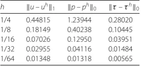
Table 3 The illustration of the error for the Oseen viscoelastic fluid flow with stabilization term for the FEp1 –p1 –p1dgtriples
h u–uh
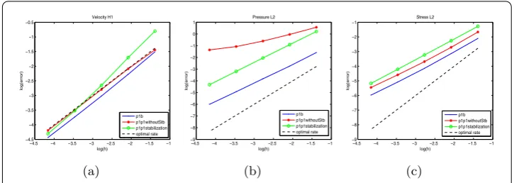
Figure 1The illustration of the order of convergence. (a)H1-norm error for velocity; (b)L2-norm error for pressure; (c)L2-norm error for stress
triples. Table2demonstrates the results for the approximation of the Oseen viscoelastic fluid model by FEp1 –p1 –p1dgtriples without stabilization term. Table3shows the error
obtained from the approximate values with stabilization term by using FEp1 –p1 –p1dg
triples.
To verify the desirable feature of the method, we compare the convergence orders in Fig.1for the three methods by using thelog–logplots of the data listed in Tables1–3. The experiment shows that, for all three methods, the order of convergence of velocity and stress is optimal ashdecreases. From Tables1–3and Fig.1we can observe that the velocityH1-norm error and stressL2-norm error obtain an optimal convergence order,
whereas the pressureL2-norm error is affected without stabilization term. The accuracy
of the convergence order of the pressure is ensured by adding a stabilization term, which is illustrated in Table3. This experimental test concludes that the technique we have adopted can be applied successfully for the Oseen viscoelastic fluid flow model.
5.2 The viscoelastic cavity flow
In this test, we apply the stabilization method in the famous problem for testing numerical validity is known as the “lid-driven cavity.” The aforementioned problem is chosen because some standard data are available for comparison. Cavity flows has been used in many test cases for testing the incompressible fluid dynamics algorithm for the Stokes flow [52]. To investigate the pressure oscillation, we perform the viscoelastic cavity flow experiment for standard FEp1b–p1 –p1dgtriples, FEp1 –p1 –p1dgtriples without stabilization, and FE
p1 –p1 –p1dgtriples with stabilization. Moreover, we compare the pressure lines of lowest
equal-order triples with standard FE methods.
The fluid is enclosed in a unit square domain with the boundary condition for velocity
u= (1, 0) on the upper boundary and the homogeneous Dirichlet condition on the re-maining boundaries. The parameters value are chosen as follows:a= 0,λ= 5.0, f = 0, and
α= 0.5. In this numerical formulation, b(x) denotes a known vector function used to lin-earize the nonlinear viscoelastic fluid flow model into reduced Oseen model equations. We output the data by computing the velocity vector field u = (u1,u2) for there different
FE triples known asp1b–p1 –p1dgstandard or MINI elements,p1 –p1 –p1dgwithout
stabilization, andp1 –p1 –p1dgwith stabilization. Furthermore, the computed solution
u= (u1,u2) is used as the known solution b(x) = (b1,b2) to reduce the nonlinear term as
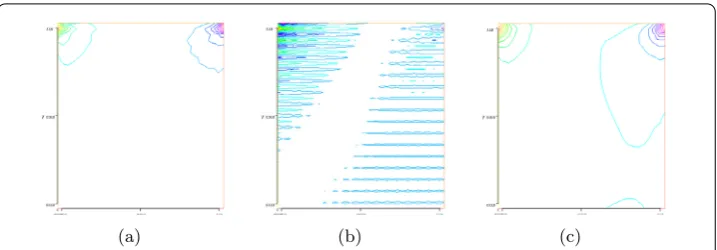
Figure 2The pressure lines for the Oseen viscoelastic cavity flow. (a) Standard FEp1b–p1 –p1dgtriples;
(b) FEp1 –p1 –p1dgtriples without stabilization term; (c) FEp1 –p1 –p1dgtriples with stabilization term
Figure 3The 4-to-1 contraction domain with sample contraction mesh
Figure2(a) represents a standard method for the approximation of the mixed FE triples
p1b–p1 –p1dg, where the pressure lines on the top corners are regular. For comparison of
the lowest equal order, we present the numerical result in Fig.2(b) without addition of a stabilization term. It can be seen that the pressure is poorly oscillated and obtain irregular shape. It is easy to observe that after adding a stabilization term in Fig.2(c), the pressure lines are appeared in similar precision with Fig.2(a). Based on this experiment, it is clear that the stabilization term ensures the stability of the scheme for the lowest equal-order triples to the approximation of the Oseen viscoelastic fluid flow model.
5.3 The 4-to-1 contraction channel flow
The third example is the well-known benchmark problem for viscoelastic fluid flow “4-to-1 contraction channel flow problem,” which has enormous application in polymeric liquid industries. The 4-to-1 channel flow has been extensively used to show the con-vergence, stability, behavior of the streamlines of the contraction channel, and the be-havior of pressure [10,24,53]. The domain of this problem is constructed in such a way that the channel lengths are sufficiently long for a fully developed Poiseuille flow at both inflow and outflow boundaries. Similar to our experiment, the diagram of the flow ge-ometry is demonstrated in Fig. 3. The computations are performed on a uniformly re-fined version of the mesh shown in Fig.4withxmin= 0.0625 andymin= 0.015625, with
Γin={(x,y) :x= 0, 0≤y≤1}andΓout={(x,y) :x= 8, 0≤y≤0.25}. For the velocity inflow
in the boundary and velocity outflow in the boundary, it is declared by
u1=
1 32
1 –y2, u2= 0 onΓin,
u1= 2
1 16–y
2
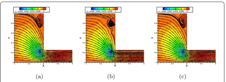
Figure 4Streamlines and magnitudes of the velocityu. (a) Standard FEp1b–p1 –p1dgtriples; (b) FE
p1 –p1 –p1dgtriples without stabilization term; (c) FEp1 –p1 –p1dgtriples with stabilization term
For stress, onΓin,
σ11=
–αλ(a+ 1)(–y/16)2
(a2– 1)λ2(–y/16)2– 1,
σ12=σ21=
–α(–y/16) (a2– 1)λ2(–y/16)2– 1,
σ22=
–αλ(a– 1)(–y/16)2
(a2– 1)λ2(–y/16)2– 1.
Symmetry conditions for the velocity on the solid walls of the concentration are imposed at the bottom of the computational domain. No-slip boundary condition is assumed in the other boundaries of the contraction channel. Besides, the physical parametersα,λ, andaare sequentially chosen 1, 8/9, 0.7, and 1. Furthermore, we computeb1 andb2by
following the procedure similar to that mentioned in Sect.5.2. This formulation have three cases in this section, namely,p1b–p1 –p1 standard,p1 –p1 –p1dgwithout stabilization,
andp1 –p1 –p1dgwith stabilization. For all cases, we use the solution ofu1andu2as the
known solution ofb1andb2to compute the approximate solution.
Figure4(a) illustrates the streamlines and flow speed of the standard FE triplesp1b–p1 –
p1dg. Figure4(b) shows the streamlines without stabilization term for the FE triplesp1 –
p1 –p1dg, and Fig.4(c) presents the streamlines with stabilization term for the FEp1 –p1 –
p1dgtriples. We can observe that without the addition of the stabilization term as shown
in Fig.4(b), the approximate value of the streamlines and vortex for the FEp1 –p1 –p1dg
triples is different and shows some irregularities. However, Fig.4(a) and Fig.4(c) appear similar in manner. The behavior of the streamlines and vortex confirm the theoretical results for the approximation of the Oseen viscoelastic fluid flow with the lowest equal-order FE triples.
In Fig.5(a), we plot the pressure contours with standard Galerkin FE known asp1b–
p1 –p1dg. To check the validity of the stabilization term, we plot the data without adding
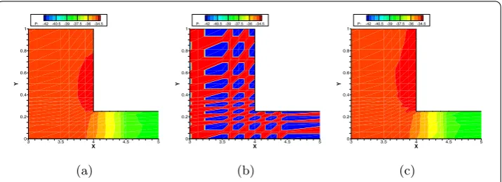
Figure 5The pressure contours for pressure fieldp. (a) Standard FEp1b–p1 –p1dgtriples; (b) FE
p1 –p1 –p1dgtriples without stabilization term; (c) FEp1 –p1 –p1dgtriples with stabilization term
stabilization under the lowest equal-order FE triples for the approximation of the Oseen viscoelastic fluid flow.
6 Conclusion and future work
In this contribution, a stabilized method for lowest equal-order finite elements (FE) triples
p1 –p1 –p1dgfor the Oseen viscoelastic fluid flow is presented. In the standard Galerkin
finite element method, the inf–sup (or LBB) condition is substantial while we circumvent the difficulty for the FE triplesp1–p1–p1dgby adding a stabilization term essentially in the
Oseen viscoelastic fluid flow model. This technique is new for the lowest equal-order FE triples for the reduced linearized viscoelastic fluid flow model. We proposed a stabilized FE algorithm and derived the well-posedness of the scheme. The desired error estimate is proved, and the optimal convergence order is obtained. In support of the given method, three numerical tests have been successfully implemented. In the analytical solution test, we demonstrate the optimal convergence order for lowest equal order. The second exper-iment elucidates the viscoelastic cavity flow to show the characteristics of the pressure contour and its behavior. The flow speed, behavior of the contours, streamlines patterns, and the pressure oscillation are examined by the “4-to-1 contraction channel flow.” This method can be extended to the streamline-upwind Petrov–Galerkin (SUPG) method for approximation of the Oseen viscoelastic fluid flow in the future studies.
Acknowledgements
The authors would like to thank the Editor and reviewers for constructive comments, which have helped to enrich the content and improve the presentation of the results in this manuscript.
Funding
This work was supported by the NSF of China with Grant Nos. 11571115, 11171269 and 11201369, Science and Technology Commission of Shanghai Municipality Grant No. 18dz2271000.
Competing interests
The authors declare that they have no competing interests.
Authors’ contributions
All authors contributed equally to this work. The manuscript is approved by all authors for publication.
Author details
1School of Mathematical Sciences, Shanghai Key Laboratory of Pure Mathematics and Mathematical Practice, East China
Normal University, Shanghai, P.R. China.2Department of Mathematics, Faculty of Science, Comilla University, Comilla,
Publisher’s Note
Springer Nature remains neutral with regard to jurisdictional claims in published maps and institutional affiliations.
Received: 21 June 2018 Accepted: 4 December 2018
References
1. Johnson, C., Pitkäranta, J.: An analysis of the discontinuous Galerkin method for a scalar hyperbolic equation. Math. Comput.46, 1–26 (1986)
2. Oldroyd, J.G.: On the formulation of rheological equations of state. Proc. R. Soc. Lond. A200, 523–541 (1950) 3. Martin, R., Zinchenko, A., Davis, R.H.: A generalized Oldroyd’s model for non-Newtonian liquids with applications to a
dilute emulsion of deformable drops. J. Rheol.58, 759–777 (2014)
4. Johnson, M.W., Segalman, D.: A model for viscoelastic fluid behavior which allows non-affine deformation. J. Non-Newton. Fluid Mech.2, 255–270 (1977)
5. Bonito, A., Clément, P., Picasso, M.: Mathematical and numerical analysis of a simplified time-dependent viscoelastic flow. Numer. Math.107, 213–255 (2007)
6. Phan-Thien, N., Tanner, R.I.: A new constitutive equation derived from network theory. J. Non-Newton. Fluid Mech.2, 353–365 (1977)
7. Renardy, M.: Mathematical Analysis of Viscoelastic Flows. SIAM, Philadelphia (2000)
8. Sandri, D.: Finite element approximation of viscoelastic fluid flow: existence of approximate solutions and error bounds. Continuous approximation of the constraints. SIAM J. Numer. Anal.31, 362–377 (1994)
9. Girault, V., Wheeler, M.F.: Discontinuous Galerkin methods. In: Partial Differential Equations, pp. 3–26. Springer, Dordrecht (2008)
10. Mahbub, M.A.A., Hussain, S., Nasu, N.J., Zheng, H.B.: Decoupled scheme for non-stationary viscoelastic fluid flow. Adv. Appl. Math. Mech.10, 1–36 (2018)
11. Lee, H.: A multigrid method for viscoelastic fluid flow. SIAM J. Numer. Anal.42, 109–129 (2004)
12. Barrenechea, G.R., Castillo, E., Codina, R.: Time-dependent semi-discrete analysis of the viscoelastic fluid flow problem using a variational multiscale stabilized formulation. IMA J. Numer. Anal. (2018).
https://doi.org/10.1093/imanum/dry018
13. Reed, W.H., Hill, T.R.: Triangular mesh methods for the neutron transport equation. Tech. report, 73–479, Los Alamos Scientific Laboratory (1973)
14. Lesaint, P., Raviart, P.A.: On a finite element method for solving the neutron transport equation. In: de Boor, C. (ed.) Mathematical Aspects of Finite Elements in Partial Differential Equations, pp. 89–123. Academis Press, New York (1974)
15. Fortin, M., Fortin, A.: A new approach for the FEM simulation of viscoelastic flows. J. Non-Newton. Fluid Mech.32, 295–310 (1989)
16. Barnger, J., Sandri, D.: Finite element approximation of viscoelastic fluid flow: existence of approximate solutions and error bounds I. Discontinuous constraints. Numer. Math.63, 13–27 (1992)
17. Zheng, H.B., Yu, J.P., Shan, L.: Unconditional error estimates for time dependent viscoelastic fluid flow. Appl. Numer. Math.119, 1–17 (2017)
18. Braack, M., Burman, E., John, V., Lube, G.: Stabilized finite element methods for the generalized Oseen problem. Comput. Methods Appl. Mech. Eng.196, 853–866 (2007)
19. Ervin, V.J., Lee, H., Ntasin, L.N.: Analysis of the Oseen-viscoelastic fluid flow problem. J. Non-Newton. Fluid Mech.127, 157–168 (2005)
20. Guillopé, C., Saut, J.C.: Existence results for the flow of viscoelastic fluids with a differential constitutive law. Nonlinear Anal.15, 849–869 (1990)
21. Luo, X.L.: An incremental difference for viscoelastic flows and high resolution FEM solution at high Weissenberg numbers. J. Non-Newton. Fluid Mech.79, 57–75 (1998)
22. Zhang, Y.Z., Xu, C., Zhou, J.: Convergence of a linearly extrapolated BDF2 finite element scheme for viscoelastic fluid flow. Bound. Value Probl.2017, 140 (2017)
23. Jenkins, E., Lee, H.: A domain decomposition method for Oseen-viscoelastic flow equations. Appl. Math. Comput. 195, 127–141 (2008)
24. Nasu, N.J., Mahbub, M.A.A., Hussain, S., Zheng, H.B.: Two-level finite element approximation for Oseen viscoelastic fluid flow. Mathematics6, 71 (2018)
25. Wang, A., Zhao, X., Qin, P., Xie, D.: An Oseen two level stabilized mixed finite element method for the 2D/3D stationary Navier–Stokes equations. Abstr. Appl. Anal.2012, Article ID 520818 (2012)
26. Lee, H.C., Lee, H.: Analysis and finite element approximation of an optimal control problem for the Oseen viscoelastic fluid flow. J. Math. Anal. Appl.336, 1090–1106 (2007)
27. Baijens, F.P.T.: Mixed finite element methods for viscoelastic flow analysis: a review. J. Non-Newton. Fluid Mech.79, 361–385 (1998)
28. Brown, R., Szady, M., Northey, P., Aramstrong, R.: On the numerical stability of mixed finite element methods for viscoelastic flows governed by differential constitutive equations. Theor. Comput. Fluid Dyn.5, 77–106 (1993) 29. Bochev, P.B., Dohrmann, C.R., Gunzburger, M.: Stabilization of low order mixed finite elements for the Stokes
equations. SIAM J. Numer. Anal.44, 82–101 (2006)
30. Brezzi, F., Fortin, M.: Mixed and Hybrid Finite Element Methods. Springer Series in Computational Mathematics. Springer, New York (1991)
31. Brezzi, F., Fortin, M.: A minimal stabilization procedure for mixed finite element methods. Numer. Math.89, 457–491 (2001)
32. Li, J., He, Y.: A stabilized finite element method based on two local Gauss integration for the Stokes equation. J. Comput. Appl. Math.214, 58–65 (2008)
33. He, Y., Li, J.: A stabilized finite element method based on local polynomial pressure projection for the stationary Navier–Stokes equations. Appl. Numer. Math.58, 1503–1514 (2008)
35. Li, R., Li, J., Chen, Z., Gao, Y.: A stabilized finite element method based on two local Gauss integrations for a coupled Stokes–Darcy problem. J. Comput. Appl. Math.292, 92–104 (2016)
36. Baranger, J., Wardi, S.: Numerical analysis of a FEM for a transient viscoelastic flow. Comput. Methods Appl. Mech. Eng. 125, 171–185 (1995)
37. Najib, K., Sandri, D.: On a decoupled algorithm for solving a finite element problem for the approximation of viscoelastic fluid flow. Numer. Math.72, 223–238 (1995)
38. Bird, R.B., Armstrong, R.C., Hassager, O.: Dynamics of Polymeric Liquids. Wiley, New York (1987)
39. Fernández-Cara, E., Guillén, F., Ortega, R.R.: Mathematical modeling and analysis of viscoelastic fluids of the Oldroyd kind. In: Handbook of Numerical Analysis, pp. 543–661. North-Holland, Amsterdam (2002)
40. Guillopé, C., Saut, J.C.: Existence results for the flow of viscoelastic fluids with a differential constitutive law. Nonlinear Anal.15, 849–869 (1990)
41. Adams, R.A.: Sobolev Space. Pure and Applied Mathematics, vol. 65. Academic Press, New York (1975) 42. Sandri, D.: Finite element approximation of viscoelastic fluid flow: existence of approximate solutions and error
bounds. Continuous approximation of the stress. SIAM J. Numer. Anal.31, 362–377 (1994)
43. Marchal, J.M., Crochet, M.J.: A new mixed finite element for calculating viscoelastic flow. J. Non-Newton. Fluid Mech. 26, 77–114 (1987)
44. Ervin, V.J., Lee, H.: Defect correction method for viscoelastic fluid flows at high Weissenberg number. Numer. Methods Partial Differ. Equ.22, 145–164 (2006)
45. Jia, H., Li, K., Liu, S.: Characteristic stabilized finite element method for the transient Navier–Stokes equations. Comput. Methods Appl. Mech. Eng.199, 2996–3004 (2010)
46. Li, Z., Chen, S., Qu, S., Li, M.: Stabilization of low-order mixed finite elements for the plane elasticity equations. Comput. Math. Appl.73, 363–373 (2017)
47. He, Y.N., Xie, C., Zheng, H.B.: A posteriori error estimate for stabilized low-order mixed FEM for the Stokes equations. Adv. Appl. Math. Mech., 798–809 (2010)
48. Zheng, H.B., Hou, Y.R., Shi, F.: A posteriori error estimate of stabilization of low-order mixed finite elements for incompressible flow. SIAM J. Sci. Comput.32, 1346–1364 (2010)
49. Zheng, H.B., Hou, Y.: A quadratic equal-order stabilized method for Stokes problem based on two local Gauss integration. Nonlinear Anal.26, 180–1190 (2009)
50. Hecht, F.: FreeFEM++. J. Numer. Math.20, 251–265 (2012)
51. Zhang, Y., Hou, Y., Mu, B.: Defect correction method for time dependent viscoelastic fluid flow. Int. J. Comput. Math. 88, 1546–1563 (2011)
52. Zheng, H.B., Hou, Y., Shi, F., Song, L.: A finite element variational multiscale method for incompressible flows based on two local Gauss integrations. J. Comput. Phys.228, 5961–5977 (2009)