R E S E A R C H
Open Access
eOLLA: an enhanced outer loop link
adaptation for cellular networks
Francisco Blanquez-Casado
*, Gerardo Gomez, Maria del Carmen Aguayo-Torres
and Jose Tomas Entrambasaguas
Abstract
Link adaptation (LA) process is a core feature for the downlink of 3GPP long-term evolution (LTE) and LTE-advanced (LTE-A). Through a channel quality indicator (CQI), the receiver suggests to the base station (BS) an appropriate modulation and coding scheme (MCS) according to the current channel conditions. In order to overcome any non-ideality in this process, the outer loop link adaptation (OLLA) algorithm is used to adaptively modify the mapping from signal-to-noise ratio (SNR) to CQI. OLLA basically modifies the measured SNR by an offset, according to whether data packets are received correctly or not, in order to adjust the average block error rate (aBLER) to a target. Although the OLLA technique has been extensively used, there exists a lack of analysis in the literature about its dynamics and convergence conditions. In this paper, a deep analysis of this algorithm has been carried out in order to cover this gap. From this analysis, we propose a new approach to the OLLA, the enhanced OLLA (eOLLA), which is able to adaptively modify its step size as well as to update its offset according to the reception conditions even if no data packets have been received. Thus, for LTE- and LTE-A-realistic scenarios, simulation results show that the proposed eOLLA outperforms the traditional OLLA, achieving a performance gain of up to a 15 % in terms of throughput. Keywords: Link adaptation, AMC, LTE-A, OLLA, BLER
1 Introduction
The adaptive modulation and coding (AMC) process car-ried out in the link adaptation (LA) is a crucial part of current wireless communication systems. This technique allows to increase the data rate that can be reliably trans-mitted [1] and has been adopted as a core feature in cellular standards such as long-term evolution (LTE) and LTE-advanced (LTE-A) [2].
In the LTE and LTE-A downlink AMC procedure [2], the user equipment (UE) has to suggest to the base sta-tion (BS) an appropriate modulasta-tion and coding scheme (MCS) to be used in the next transmission in order to keep the block error rate (BLER) below a target. The pro-posed MCS is signaled from the UE by means of a channel quality indicator (CQI). Typically, each CQI is associ-ated with a particular signal-to-noise ratio (SNR) inter-val; hence, MCSs are selected by mapping the estimated instantaneous SNR into its corresponding SNR interval, defined by an upper and a lower threshold.
*Correspondence: [email protected]
Department of Communications Engineering, Universidad de Málaga, Malaga, Spain
A static selection of the values for the AMC thresholds does not perform well in practical implementations as link conditions are inherently variant. It is usual to adjust these thresholds by means of the well-known outer loop link adaptation (OLLA) technique, which was first proposed in [3]. Basically, OLLA modifies the SNR thresholds by an offset [4, 5] which can be positive (making the MCS selec-tion more robust) or negative (when the CQI selecselec-tion was too strict). This offset is continuously updated based on the reliability of the received data blocks so that the average BLER is kept as close as possible to a predefined target.
Although there are works devoted to OLLA in the lite-rature [6, 7], they typically address its performance from simulations, and the lack of a comprehensive analysis of its behavior in the literature is noticeable. Furthermore, to the best of our knowledge, previous works do not analyze the conditions under which the OLLA technique works properly. The first aim of this work is to cover this gap by carrying out a deep study of the OLLA technique.
From this study, improvements in the implementation of the traditional OLLA can be inferred. Thus, in this
paper, a different approach to the OLLA technique is pro-posed, the enhanced OLLA (eOLLA), which can signifi-cantly improve the performance of the traditional OLLA.
This paper is organized as follows. In Section 2, the AMC model for LTE used in this work is described, and then a detailed description of the OLLA is carried out, including a study of its convergence conditions and its per-formance. In Section 3, the proposed eOLLA is presented. Finally, Section 4 shows a comparison between both the traditional OLLA and the proposed eOLLA in realistic scenarios based on the downlink of LTE and LTE-A, and some concluding remarks are given in Section 5.
2 Outer loop link adaptation (OLLA)
To perform the AMC [1], the instantaneous SNRγ is esti-mated at the UE to determine the current fading regioni
and, consequently, the transmission rateRi(bits/symbol).
At the UE, this instantaneous SNR is mapped into a certain CQI value, which is fed back to the BS.
The set of SNR thresholds{i}i=0,1,..,ndefines the
inter-vals to map the estimated instantaneous SNR into its corresponding CQI, with0representing the minimum
required SNR for transmission (outage condition) and n = ∞. These thresholds have been designed in order
to accomplish certain constraints, such as limiting the maximum instantaneous BLER (iBLER) or defining an average BLER (aBLER) target. The latter approach (based on aBLER) is the one adopted by most wireless tech-nologies like LTE [1]. Therefore, our description will be focused on the aBLER scenario.
For a certain average SNR, the average BLER under AMC can be evaluated as
aBLER(,{i})=
being iBLERAWGNi (γ ), the instantaneous BLER for a given MCS i over an additive white Gaussian noise (AWGN) channel and po(,γ ) the probability density function (PDF) of the instantaneous SNR conditioned to transmission.
In this, work we have assumed an uncorrelated Rayleigh channel for the analysis. Thus, the PDF of the instanta-neous SNR for a certain average SNR is given by an exponential function [1]
p(,γ )= 1
e−γ/. (2)
Then, the instantaneous SNR conditioned to transmis-sion is given by:
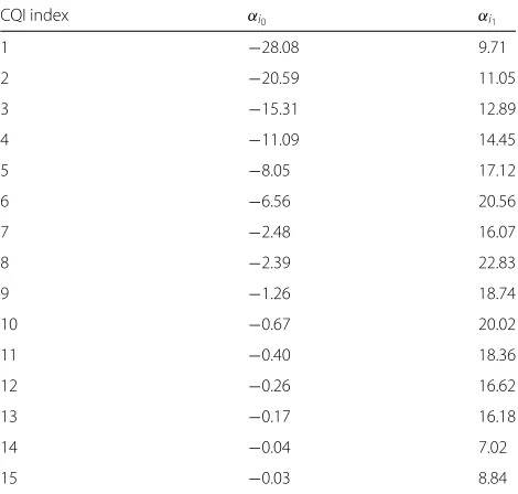
po(,γ )= According to Eq. (1), in order to evaluate the aBLER, it is necessary to have at our disposal an expression for iBLERAWGNi , but to the best of our knowledge, this is not available in the literature when turbo coding is used. Moreover, the exact value of the iBLER strongly depends on the specific decoder implementation [8]. Nevertheless, since the iBLER metric represents the probability of being in one of two states{error,no−error}, we propose the use of binary logistic regression [9]. This regression is a binary classifier based on one or more input variables. Thus, it is a useful tool to model iBLER curves for each MCS i over AWGN channels, for a given instantaneous SNRγ, by means of binary logistic functions as:
iBLERAWGNi (γ )≈fi(γ )=
1
1+e−αi0γ−αi1, (5) where the αi0 and αi1 values (see Table 1) are to be
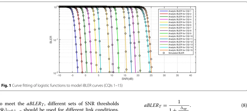
found from the logistic regression over results of the actual decoder implementation (see Section 3.2 for fur-ther details). The accuracy of logistic functions after the curve-fitting process is shown in Fig. 1 for the whole set of CQI values of LTE [2], where solid lines represent the analytic BLER curves whereas simulation results of a soft output Viterbi algorithm (SOVA)-based turbo decoder [10] are marked with circles.
A static selection of the values for the AMC thresh-olds i does not perfectly adjust the aBLER to a target
since link conditions are inherently variant. Thus, in order
SNR(dB)
-10 -5 0 5 10 15 20 25 30 35 40
BLER
10-2
10-1 100
Analytic BLER for CQI 1 Analytic BLER for CQI 2 Analytic BLER for CQI 3 Analytic BLER for CQI 4 Analytic BLER for CQI 5 Analytic BLER for CQI 6 Analytic BLER for CQI 7 Analytic BLER for CQI 8 Analytic BLER for CQI 9 Analytic BLER for CQI 10 Analytic BLER for CQI 11 Analytic BLER for CQI 12 Analytic BLER for CQI 13 Analytic BLER for CQI 14 Analytic BLER for CQI 15 Simulated BLER
Fig. 1Curve fitting of logistic functions to model iBLER curves (CQIs 1–15)
to meet the aBLERT, different sets of SNR thresholds
{i}i=0,1,..,n should be used for different link conditions.
This can be modeled by rewriting each SNR threshold i = γi·θ, beingγian initial value, andθ an offset that
must be designed to meet the aBLERT. Then, Eq. (1) is
modified as
aBLER(,{γi},θ)= n−1
i=0 γi+1θ
γiθ
iBLERAWGNi (γ )p(γ )dγ.
(6)
The previous process is typically performed in prac-tical implementations by the outer loop link adaptation (OLLA) technique [3–5]. The traditional OLLA opera-tion consists in dynamically modifying the value of the offset according to whether the previously transmitted data packet has been correctly received or not. In LTE and LTE-A, this information is extracted from the cyclic redundancy code (CRC) [11]. Thus, OLLA can be seen as a discrete time system in which, each timeka CRC is received, the value of the offsetθ[k] is updated according to the following equation [5]
θdB[k]=θdB[k−1]+up·e[k]−down·(1−e[k]),
(7)
being
• θdB[k]=10·log10(θ[k]).
• e[k]an error indicator, whose value is 0 if the CRC is correct, or 1 if not. It corresponds to a dichotomous random variable whose average is the aBLER. • upanddownconstant increment and reduction
values, respectively, of the offset, in decibels. These two values are positive and should satisfy Eq. (8) in order to meet theaBLERT[5]. This condition will be
justified in Subsection 2.1.
aBLERT =
1
1+up down
. (8)
In addition to that, the value ofdowncannot exceed an
upper limitdownmax in order to ensure the proper work-ing of the OLLA. This limit is given by the next equation, which is justified in Subsection 2.1.
downmax <
2e·aBLERT
−α1
. (9)
SNR threshold values are now modified at each instant kby a discrete offset, so they can be expressed as
i[k]=γi·θ[k] . (10)
To sum up, the OLLA operation consists in increas-ing the offset value (and so increasincreas-ing the value of the SNR thresholds) when error happens, and decreasing them when transmissions are correct. Therefore,θ[k] val-ues higher than 1 increase transmission robustness, while values lower than 1 decrease it.
2.1 OLLA convergence in average
It should be noticed that OLLA dynamics imply that the offset valueθdB[k] is continuously being updated by
addingup(if error) or subtractingdown(if not). Thus, it
will never converge to a single value. However, the offsetθ presented in (6) is a single value that ensures theaBLERT
for stationary link conditions. The reason of this differ-ence is thatθis used in an averaging process, while in case of the OLLA,θdB[k] is an instantaneous value. Therefore,
to study the convergence of the OLLA process, averaged values must be considered.
E[θdB[k]] = θdBk value at k, obtaining the following
Note that since the average value of θdB[k] depends
on k, it is not an ergodic process. Only when k → ∞ the process can be considered ergodic. Expression (11) corresponds to a difference equation, i.e., there is a recur-rence relation between the terms in the form ofθdBk = TθdBk−1
, beingT(θdB)the recurrence function. Hence,
according to the Banach fixed-point theorem [12], when k → ∞ the equation will converge to the only value such thatθdBo = TθdBo if certain conditions are fulfilled. The following equation is obtained when convergence in average is reached the aBLER. Thus, in order to ensure that the converged offset valueθdBo = 10·log10(θo)meets theaBLERT, the
aBLER should be forced to this value, obtaining the the following relation
which was already presented in (8), and now it has been justified. Therefore, under certain link conditions, the OLLA algorithm converges in average to a valueθowhich is the value ofθ to be introduced in (6) in order to meet theaBLERT.
Equation (13) manifests that there are infinite suit-able combinations of up and down that ensures the
aBLERT. However, the specific values of up anddown
must accomplish the convergence criteria required by the Banach fixed-point theorem applied to (11), whose two sufficient conditions are described next.
2.1.1 First Banach fixed-point theorem condition
The function T(θdB) should be a contraction mapping,
that is, it should satisfy that
T(θdB)∈[θmin,θmax] ,∀θdB∈[θmin,θmax] . (14)
It can be easily shown that this condition is always ful-filled by the OLLA. Firstly, since E[e[k]] is the average number of errors, i.e., the aBLER, its range of values are comprised between 0 and 1. Thus, there will be a value θdB=θminlow enough to ensure that E [e[k]]=1, which
means thatT(θmin)=θmin+up. Then, asθdBincreases,
the value of E [e[k]] will decrease untilθdBraises a value
θmax high enough to ensure that E [e[k]] = 0, which
means thatT(θmax)= θmax−down. As a result of that,
the values ofT(θdB)will be comprised between
T(θdB)∈
2.1.2 Second Banach fixed-point theorem condition
The second condition that the function T(θdB) should
fulfill is that
T(θdB) <1, ∀θdB∈[θmin,θmax] (16)
being T(θdB) the first order derivative of T(θdB). To
check this condition, it is necessary as an expression for E [e[k]], this is, for the aBLER. This expression is pro-vided by (6), and it depends on the specific parameters of the binary logistic regression carried out to model the iBLERAWGNi curves. In order to have a more tractable expression, aBLER(,{γi},θ) values have been obtained
numerically for an average SNR value of = 15dB and certain iBLERAWGNi curves (see Section 5 for fur-ther details) for differentθdBvalues according to (3), (5),
and (6). These values have been obtained based on the parameters of Table 2 and are presented in Fig. 2 (solid line).
The shape of the aBLER curve is similar to the iBLER. Thus, it could also be modeled by means of logistic regres-sion, which was introduced in Section 2. In this case, we propose to model this curve by means of a modified binary logistic function, which introduces a parameters which controls the slope, as
E[e[k]]=aBLER(,θdB)≈fm(θdB)=
regression, the resulting fitted curve is shown in Fig. 2 as a dashed line. It can be seen how the proposed expression perfectly fits with the simulated results.
By using the proposed modified logistic function, it can be evaluated by the expression of T(θdB), according to
(11), as
T(θdB)=θdB+up+down
·fm(θdB)−down (18)
Next, the condition to ensure that T(θdB) < 1 is
derived from (13), (17), and (18). First, we find the value of T(θdB)as
Table 2Parameters for OLLA convergence
Fig. 2Curve fitting of modified logistic function to model aBLER for
0, and both up and down are positive, the following
condition must be guaranteed in order to ensure the convergence condition
imposed by (20) is fulfilled. After reordering, we find
that the offset value θdBmax for which the maximum of
fm (θdB) is achieved as
ing function implies thats ≥ 0. It can be easily seen that higher values of fm(θdB) are achieved ass is increased.
Then, we get an upper bound offm (θdB)whens→ ∞as
fmmax = |α1|
e . (23)
Finally, from (13), (20), and (23), we find that the second condition to ensure the OLLA convergence, which was already presented in (9), is given by
downmax <
2e·aBLERT
−α1
.
Thus, convergence is ensured if the decrement step does not raise a maximum value, which is determined byα1,
that is, by the curve of aBLER for a certainvalue of mean SNR.
According to previous results, there is a range ofdown
values, and so ofup values, that ensures convergence.
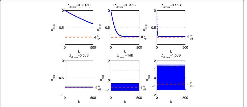
In Fig. 3, the convergence process when different values ofdownare used is presented, for given link conditions
whose parameters are listed in Table 2. These parameters have been obtained for the same conditions in Fig. 2.
Figure 3, shows how the converged valueθdBk raises its final valueθdBo ≈ −0.8 (dashed line) faster as the size of
down is higher. Note that this convergence value is the
same that obtained in Fig. 2 by using (17). Oncedown
exceeds downmax, whose value is 0.52 for the proposed scenario, the OLLA begins to diverge, this divergence being more remarkable asdown increases. Therefore, it
would be advisable to choose the highest possible value of downin order to achieve convergence as fast as possible.
2.2 OLLA performance
In this subsection, the OLLA performance is analyzed under stationary link conditions. As it will be shown, when convergence, the instantaneous offset valueθdB[k]
fluctuates around the converged valueθdBo following the instantaneous channel variations. The amplitude of these fluctuations will be related to the values ofupanddown.
Thus, high values of these two parameters, even if they guarantee the OLLA convergence, may lead to a high vari-ance in the instantaneous offset value that could degrade the OLLA performance. On the other hand, too small val-ues ofupanddownmay imply that the OLLA could not
follow the channel variations if they are too fast.
In Fig. 4, the instantaneous values of θ[k] are shown for the same simulation conditions of Table 2, for a set of values ofdownthat guarantee convergence (down < downmax = 0.52). These results show that for the lowest down value, it takes several steps to the OLLA to reach
a state for which the offset is stabilized around a certain value, which is the converged valueθdBo ≈ −0.8 of Fig. 3. As the value ofdownincreases, it takes less steps to the
OLLA to stabilize; however, the variance of the offset also increases, which may cause a degradation in the OLLA performance.
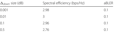
As it was previously stated, a high variance of the OLLA offset can degrade its performance. This fact is shown in Table 3, which presents the achieved throughput and
Fig. 4Instantaneous offset for an uncorrelated flat Rayleigh channel
Table 3System performance for OLLA with differentdownsizes
downsize (dB) Spectral efficiency (bps/Hz) aBLER
0.001 2.98 0.1
0.01 3 0.1
0.1 2.96 0.1
0.5 2.76 0.1
the aBLER for the differentdownvalues, under the same
condition as in Fig. 4. Results reveal that as the size of the step increases, there is a reduction of the spectral effi-ciency, although all configurations meet theaBLERT. The
reduction of spectral efficiency for the maximumdown value that guarantees convergence (0.5 dB) is about 8 % with respect to the step value with better throughput performance (down=0.01 dB).
The reason for this throughput degradation for high step values is that they may cause that when an error happens, the OLLA selects a more robust MCS than the required to ensure theaBLERT.
To sum up, while high values of the OLLA steps are desirable to achieve a fast convergence, low step values lead to higher throughput once convergence is achieved, since it provides a better adjustment of the MCS. Thus, the selection of the values of up and down should
be carried out carefully in order to optimize the OLLA performance.
3 Enhanced outer loop link adaptation
In the previous section, the traditional OLLA algorithm has been deeply studied, showing that a key factor to opti-mize the performance is the appropriate selection of its step size. However, the way this selection should be car-ried out is not clear. Moreover, the performance of the OLLA also depends on the specific implementation of features at the receiver such as the turbo decoder or the channel estimation method.
In addition to that, another problem is that the OLLA only updates its offset every time k an ACK/NACK is received, i.e., when a transmission is done. In real sce-narios, it is usual not to have full-buffer traffic but a discontinuous transmission with variable traffic. In these cases, the UE may be most of the time in idle mode [13]. Therefore, a combination of variant channel conditions together with these kind of traffic patterns could cause a performance degradation since the OLLA may not be able to update its offset fast enough to follow the channel variations.
3.1 Proposed eOLLA
system. Furthermore, the proposed eOLLA updates its offset independently of whether a transmission is carried out or not.
Since the error indicator e[k] used in the traditional OLLA can be seen as a one bit instantaneous BLER esti-mator (1 if error, 0 if not), this value could be replaced by a more accurate instantaneous BLER estimation. Thus, to carry out the implementation of the proposed eOLLA, a model for the instantaneous BLER of each MCSiover AWGN channels for instantaneous SNR,iBLERAWGNi (γ), is needed.
The proposed eOLLA implemented from (7) is as fol-lows
1. If an ACK/NACK is received, update the
correspondingiBLERAWGNi model according to the MCSi used in this transmission (optional). 2. Estimate the instantaneous SNR valueγ[t]. 3. At each Transmission Time Interval (TTI)t,
calculate the instantaneous BLER value B[t]=iBLERAWGNi (γ[t]).
4. Get the offset value as
θdB[t]=θdB[t−1]+up·B[t]−down·(1−B[t]). (24)
In the eOLLA algorithm description, it should be noticed that the index k of Eq. (7) of the traditional OLLA description has been replaced by the index t in Eq. (24). This means that the offset of the eOLLA will be updated every TTIt (every time a transmission can be potentially carried out) instead of every timeka CRC is received (every time a transmission is carried out). Then, in case of discontinuous transmissions, the pro-posed eOLLA updates its offset more frequently than in case of the traditional OLLA, which implies that the eOLLA is able to follow easily the temporal variations of the channel, thus improving the AMC performance.
This continuous updating of the eOLLA offset can be easily performed in LTE since there is an estimation of the SNR available every TTIt. In the downlink of LTE and LTE-A, the BS transmits reference signals (RS) [2] at each subframe, in both connected and idle modes. Thus, every UE is able to perform SNR estimation from this RS at each TTI, and so to update its eOLLA offset.
The fitting process referred in step (1) of the proposed algorithm is used to adjust the instantaneous BLER model to the specific system implementation used. This process is required just in case a fitted model is not available.
For the purpose of a better understanding of the eOLLA behavior, step (4) can be rewritten according to (13) as
θdB[t]=θdB[t−1]+down·
From the previous equation, it can be deduced that the proposed eOLLA adapts the increment to be applied to
the offset according to the difference between the esti-mated instantaneous BLER B[t] and the target aBLER. Then, ifB[t]= 0, the offset will be decreased bydown,
thus decreasing the robustness of the next transmission in the same way than in the traditional OLLA. As B[t] increases, the size of the decreasing step reduces, and so increases the robustness of the next transmission until B[t]= aBLERT, which is the equilibrium point. At this
point, no step will be applied to the offset, since if the eOLLA remains in this state the average BLER will meet the target aBLER. In case thatB[t] exceeds theaBLERT,
the offset will be increased, and thus the robustness of the next transmission, untilB[t]= 1. In this case, the offset will be increased byup, as in the traditional OLLA.
Hence, for the eOLLA, if the offset value leads to either a very high or a very low instantaneous BLER, high-step values are used in order to correct this situation as fast as possible. Then, as the iBLER is closer to the average target BLER, lower step sizes are used to reduce the variance of the MCS and maximize the throughput.
SinceE[B[t]] is the same thanE[e[t]], the convergence analysis of the traditional OLLA carried out in Subsection 2.1 can be applied to the eOLLA. Thus, to ensure the convergence of the eOLLA, condition (9) must be also sat-isfied. Note that under stationary conditions, the offset value for which E[B[t]] = aBLERT corresponds to the
convergence valueθdBo previously described.
3.2 Logistic regression implementation
In previous section, we stated that an expression of the instantaneous BLER iBLERAWGNi (γ[t]) was required to model the eOLLA algorithm. As described in Section 2, instantaneous BLER for MCSiover AWGN channels can be modeled by means of binary logistic functions.
Therefore, logistic regression can be used in the eOLLA algorithm (step 1) to find out the values ofαi0 andαi1
in Eq. (5) that better fit with the iBLERAWGNi curve. In practice, this logistic regression can be easily implemented by the well-known gradient descend algorithm [14]. This algorithm is typically used to minimize a cost function J(α)as follows
α:=α−λ ∂
∂αJ(α) (26)
where λ is a parameter that controls the convergence speed. Thus, first of all, it is necessary to provide the logistic regression cost function, given by [15]
J(α)=y·logfα(x)−(1−y)·log1−fα(x) (27)
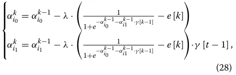
instantaneous SNR valueγ, the classification resultyas an error indicatore, andfα as the binary logistic function of (5). Then, applying partial derivation of the cost function, the resulting logistic regression process for the proposed eOLLA is given by:
⎧ packet at the instant k, which is obtained from the ACK/NACK report, andγ[t−1] is the estimated instan-taneous SNR during the previous TTI t. Note that the values ofαik0 andαik1 have to be updated simultaneously. Regardingλ, low values will lead to a slower but a more accurate convergence, while high values will accelerate the convergence, although it may also cause oscillations. However, it should be noticed that the logistic regression cost function is convex, so convergence is guaranteed.
3.3 eOLLA performance
Figure 5 shows the instantaneous offset valueθ[t] of the eOLLA for the same conditions as that in Fig. 4. Note that in this case,t=ksince a transmission is carried out every TTI. In this figure, it can be seen that the convergence values are the same with that achieved for the traditional OLLA. In addition, instantaneous offset values have lower variance than the ones obtained in Fig. 4 for the same down.
Fig. 5Instantaneous offset for an uncorrelated flat Rayleigh channel
Throughput and aBLER results are shown in Table 4. For the eOLLA, an increment ofdowndoes not lead to
an important throughput degradation as in the case of the traditional OLLA (see Table 3). The throughput degra-dation when using the highestdownconsidered in these
simulations is about 4 % for the eOLLA, while for the tra-ditional OLLA, this degradation is doubled. In both cases, theaBLERT is met.
Results presented for the traditional OLLA and the eOLLA do not correspond to a realistic scenario, since an uncorrelated channel is assumed. However, they are useful in order to understand the dynamics of both the OLLA and the proposed eOLLA. In practice, AMC can-not be used in uncorrelated channels due to the outdating of CQI reports. Next, both OLLA and eOLLA have been evaluated in a correlated channel scenario. Furthermore, a bursty traffic pattern has been taken into account in order to give a complete picture.
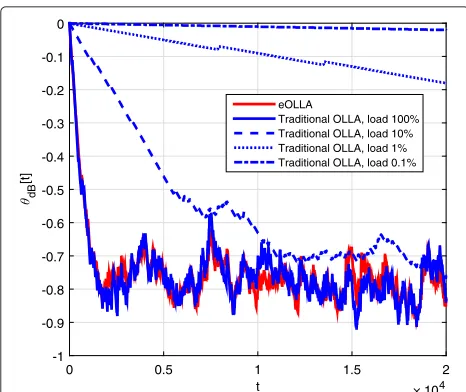
Figure 6 shows the instantaneous offset values for both the traditional OLLA and the eOLLA for a correlated flat Rayleigh channel with a Doppler frequency (fD) of 7 Hz
andaBLERT =0.1, when a smalldownstep is used (0.001
dB). The transmission periods are expressed in percent-age of the maximum traffic load case. First of all, notice that the same results are achieved by the eOLLA inde-pendently of the traffic load, since the eOLLA only needs the estimated iBLER (available at each TTI) to update the offset. In contrast, different performance is achieved by the traditional OLLA depending on the traffic load, since it needs an ACK/NACK report to update its state. As a consequence, when full buffer is assumed, i.e., t = k, both OLLA implementations have a similar performance; but as the traffic load decreases, it is harder for the tra-ditional OLLA to follow the temporal channel variations since its offset is only updated when a CRC is received, thus degrading its performance compared to the eOLLA, which updates its offset every TTI.
On the other hand, if the same simulation is carried out with a high step sizedown =0.5, which ensures
conver-gence, this convergence is easily achieved independently of the traffic load. However, low load is still a problem for the traditional OLLA since it is not able to properly follow the channel, as shown in Fig. 7.
Table 4System performance for eOLLA with differentdown
sizes
downsize (dB) Spectral efficiency (bps/Hz) aBLER
0.001 2.99 0.1
0.01 3 0.1
0.1 2.99 0.1
Fig. 6Instantaneous offset comparison for a correlated flat Rayleigh channel (fD=7 Hz) withdown=0.001 dB
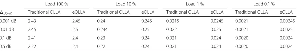
Table 5 summarizes the spectral efficiency results for different traffic loads and down sizes for both the
traditional OLLA and the eOLLA, assumingaBLERT =
0.1 and a correlated flat Rayleigh channel with fD =
7 Hz. First of all, note that for high down sizes the
performance of both OLLA techniques is degraded, inde-pendently of the traffic load. However, while this degra-dation does not exceed the 4 % for the eOLLA, in the case of the traditional OLLA, this degradation varies between 5 and 10 %. Furthermore, given a down step
size, the performance of the eOLLA does not vary with the traffic load. However, when using the traditional OLLA, low traffic load can degrade its performance with
Fig. 7Instantaneous offset comparison for a correlated flat Rayleigh channel (fD=7 Hz) withdown=0.5 dB
respect to the eOLLA up to 17 %. To sum up, the eOLLA outperforms the traditional OLLA while reduc-ing the influence of thedown step size and the traffic
load.
4 eOLLA: application and simulation scenarios The proposed eOLLA has been implemented in a com-plete 3GPP-LTE-A downlink simulator [10] in order to present realistic scenarios for which the eOLLA can significantly improve the performance of the tra-ditional OLLA. These scenarios are based on LTE and LTE-A features. Both the traditional OLLA and the eOLLA have been evaluated for different sizes of down, all of them ensuring convergence according to
Subsection 2.1.
4.1 Simulation environment
The 3GPP-LTE-A downlink simulator includes most of the features of physical (PHY) and medium access control (MAC) layers. Furthermore, it includes the LTE-A eICIC feature [16], which will be addressed in Subsection 4.5.
The MAC layer includes a hybrid automated repeat request (HARQ) process and an AMC process, which exchanges information with a channel aware scheduler. This scheduler allocates the LTE transport blocks (TBs) by assigning a set of physical resource blocks (PRBs) with a certain MCS [2] to each UE in order to meet some criteria. At the BS, the PHY layer is made up of a coder system, which includes a CRC and a turbo coder; a quadrature amplitude modulation (QAM) mapper and an orthogo-nal frequency domain multiplexing (OFDM) modem. An AWGN channel and a multipath channel with temporal fading are included. At the UE, channel estimation and SINR estimation methods are implemented. With those methods, the channel state information (CSI) is reported to the BS [2]. The CSI is composed of the CQI, the pre-coding matrix indicator (PMI) and the rank indicator (RI). A QAM demapping and a channel-decoding pro-cess, which includes a CRC decoder and turbo decoder, is carried out to obtain the transmitted TBs. Finally, a HARQ entity manages the report of the ACK/NACK to the BS.
Table 6 summarizes the main simulation parame-ters. A typical pedestrian mobile speed (3 km/h) has been assumed to ensure the evaluation of the OLLA implementations under appropriate operating condi-tions of the AMC process. Regarding the channel aware scheduling, a round robin algorithm has been selected.
4.2 High traffic load with continuous transmission scenario
Table 5Spectral efficiency (bps/Hz) comparison between traditional OLLA and eOLLA in correlated flat Rayleigh channel (fD=7 Hz)
Load 100 % Load 10 % Load 1 % Load 0.1 %
Down Traditional OLLA eOLLA Traditional OLLA eOLLA Traditional OLLA eOLLA Traditional OLLA eOLLA
0.001 dB 2.43 2.45 0.24 0.245 0.0215 0.0245 0.0021 0.00245
0.01 dB 2.45 2.5 0.244 0.25 0.022 0.025 0.0021 0.0025
0.1 dB 2.41 2.4 0.23 0.24 0.021 0.024 0.0020 0.0024
0.5 dB 2.22 2.4 0.22 0.24 0.021 0.024 0.0020 0.0024
traffic load is evaluated . In this scenario, both algorithms update their offsets continuously as there will always be queued packets to be transmitted. Then, the ben-efit of eOLLA comes from its ability to dynamically adapt the size of the step, thus reducing the offset variance.
Next, main results for BLER, throughput, goodput, mean packet delay and jitter [17] are shown for differ-ent sizes ofdown. Except for the BLER, these results are
expressed in percentage of the maximum value (which is also indicated in the figures). As shown in Fig. 8, there is no performance difference in terms of BLER since theaBLERT is met for both algorithms. However,
it can be seen in Figs. 9 and 10 that a better perfor-mance in terms of throughput and goodput is achieved by the eOLLA for the majority of down sizes. Only
for the lowest down sizes, throughput and goodput
results are quite similar since the margin of adaptation
Table 6Simulation parameters
Parameter Value
Carrier frequency 2 GHz
Sampling frequency 7.68 MHz
System bandwidth 5 MHz
FFT size 512
Number of data subcarriers 300
OFDM symbols per subframe 14
Allocable PRBs 25
Channel model Flat Rayleigh
Mobile terminal speed 3 km/h
Number of antennas 1 x 1
Channel aware scheduler algorithm Round robin
Channel estimation method Low-pass filter [21]
Interference and noise power estimation Error-based
Reference signals overhead According to 3GPP TS36.211 [2]
Turbo decoder SOVA-based
Number of CQI bits 4 [19]
Average SNR 15 dB
down 0.001–0.5 dB
of the step is very low. As the step size increases, the eOLLA gain is more remarkable, achieving a gain close to the 15 %.
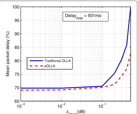
Finally, the performance in terms of delay is evalu-ated, which is a very useful metric [18]. Figures 11 and 12 show the results for mean packet delay and jitter, respectively. In this case, the eOLLA also outperforms the traditional OLLA. While for the traditional OLLA, the optimum size of down is the lowest, the eOLLA
toler-ates higher sizes without a significant degradation of its performance.
4.3 High load traffic with bursty transmission scenario
In some scenarios, it is possible that some UEs cannot be served even if they have queued packets and good chan-nel conditions, because of low-priority assignment or in case the BS is serving a great number of UEs. In this situ-ation, the UE may stay in idle mode during long periods; as a consequence, channel conditions may change consid-erably during the time interval between packets, so the offset of the traditional OLLA would be outdated (since it can only be updated when an ACK/NACK is received). However, as analyzed in previous section, the eOLLA is
10−3 10−2 10−1
0 0.02 0.04 0.06 0.08 0.1 0.12 0.14 0.16 0.18 0.2
Δdown (dB)
aBLER
Traditional OLLA eOLLA
10−3 10−2 10−1 75
80 85 90 95 100
Δdown (dB)
Throughput (%) Traditional OLLA
eOLLA Throughput
max=8.75Mbps
Fig. 9Throughput comparison for high traffic load with continuous transmission scenario
able to follow the channel variations even if no packets are received, since it uses the instantaneous SNR estimation to update its offset.
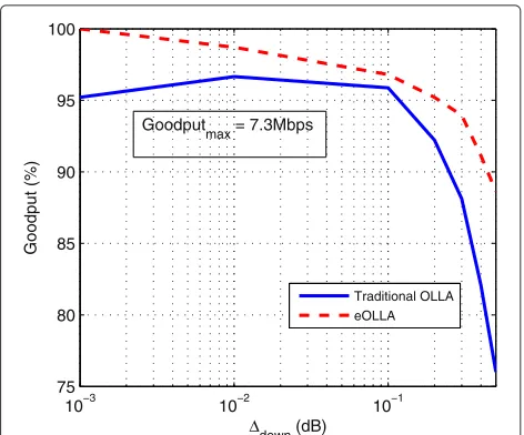
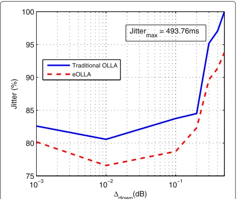
In this section, we evaluate a scenario where a data transmission is just allowed every 100 TTIs. Figures 13, 14, 15, 16, and 17 present the performance results in terms of throughput, goodput, mean packet delay, and jitter (expressed in percentage of the maximum value).
In Fig. 13, it can be seen that the traditional OLLA does not raise theaBLERT for the lowest values ofdown,
10−3 10−2 10−1
70 75 80 85 90 95 100
Δdown (dB)
Goodput (%) Traditional OLLA
eOLLA Goodput
max = 7.7Mbps
Fig. 10Goodput comparison for high traffic load with continuous transmission scenario
10−3 10−2 10−1
65 70 75 80 85 90 95 100
Δdown(dB)
Mean packet delay (%)
Traditional OLLA eOLLA
Delay
max = 931ms
Fig. 11Mean packet delay comparison for high traffic load with continuous transmission scenario
whereas the eOLLA achieves the aBLERT. The reason
is that in the traditional OLLA, the offset cannot be updated continuously in order to follow the channel. As a result, Fig. 14 shows that for the lowest step sizes, the traditional OLLA decreases its throughput dramat-ically with respect to the eOLLA, as much as 15 %. Regarding the rest of performance metrics (Figs. 15, 16, and 17), the eOLLA generally outperforms the tradi-tional OLLA while it is less influenced by the size of down. Only for the lowest values of down, delay
met-rics are pretty similar. However, since the aBLERT is
10−3 10−2 10−1
30 40 50 60 70 80 90 100
Δdown(dB)
Jitter (%) Traditional OLLA
eOLLA
Jitter
max = 1.28ms
10−3 10−2 10−1 0
0.02 0.04 0.06 0.08 0.1 0.12
Δdown (dB)
aBLER
Traditional OLLA eOLLA
Fig. 13BLER comparison for high traffic load with bursty transmission scenario
not met for the traditional OLLA, these results are not meaningful.
4.4 Low-load traffic scenario
A M2M, online gaming [18] or an automated teller machine (ATM) scenario are examples of bursty traffic patterns with low data packet rates. In such scenarios, small data packets are exchanged over long periods of time; UE during these periods of time remain in idle mode. In LTE and LTE-A, there exists a minimum number of physical resources to allocate the TB to be transmitted [19]. For the DL, this number depends on the system
10−3 10−2 10−1
80 82 84 86 88 90 92 94 96 98 100
Δdown (dB)
Throughput (%)
Traditional OLLA
eOLLA Throughput
max = 0.08Mbps
Fig. 14Throughput comparison for high traffic load with bursty transmission scenario
10−3 10−2 10−1
75 80 85 90 95 100
Δdown (dB)
Goodput (%)
Traditional OLLA eOLLA Goodput
max = 7.3Mbps
Fig. 15Goodput comparison for high traffic load with bursty transmission scenario
bandwidth; for instance, for a system bandwidth of 5 MHz the minimum number of physical resources corre-sponds to one PRB. Thus, in case that the size of the packets to be transmitted is smaller than the minimum number of assignable physical resources, more redun-dancy will be included to fill them, i.e., the MCS will be modified making it more robust than the proposed by the reported CQI. As a consequence, less erroneous TBs will be received, and therefore, the aBLER will be lower than theaBLERT, making the traditional OLLA to
increase its offset in order to meet the target aBLER. Note that in this case, the traditional OLLA is unnecessarily
10−3 10−2 10−1
90 91 92 93 94 95 96 97 98 99 100
Δdown(dB)
Mean packet delay (%)
Traditional OLLA
eOLLA
Delay
max = 2540ms
10−3 10−2 10−1 75
80 85 90 95 100
Δdown(dB)
Jitter (%)
Traditional OLLA
eOLLA
Jitter
max = 493.76ms
Fig. 17Jitter comparison for high traffic load with bursty transmission scenario
forcing the aBLER to meet the target, since increasing the robustness of the MCS does not mean saving phys-ical resources when the minimum number of assignable PRBs is used. Instead, it will cause erroneously received TB that could be avoided without increasing the amount of physical resources. Therefore, if the eOLLA is used in this scenario, since its offset is not affected by the number or erroneous TBs received but by the instanta-neous channel state, it will not try to force theaBLERTto
be met.
Next, the figures show the performance of the tradi-tional OLLA and the eOLLA for an online gaming sce-nario [20], whose mean packet size is 70 bytes and mean period between packets is 50 ms. Figure 18 shows that the average BLER is not achieved for the eOLLA whereas the traditional OLLA achieves it for the majority of thedown
sizes. Regarding the normalized throughput, 100 % is always achieved since the capacity of the system is higher than the load of the traffic source. This fact also means that packet delay is always the minimum achievable value, i.e., 1 ms. Finally, goodput results of Fig. 19 show how the eOLLA outperforms significantly the traditional OLLA without any extra cost in terms of physical resources usage.
4.5 eICIC scenario
In LTE-A, the time domain-enhanced cell inter-ference coordination (eICIC) is defined as a tech-nique to manage interference in heterogeneous networks (HetNets). An extensive description of this technique can be found in [16]. Briefly, in a scenario composed by a macro- and a pico-cell, a bias is applied to the cover-age area of the pico-cell to balance the number of users
10−3 10−2 10−1
0 0.01 0.02 0.03 0.04 0.05 0.06 0.07 0.08 0.09 0.1
Δdown (dB)
aBLER
Traditional OLLA
eOLLA
Fig. 18BLER comparison for low load traffic scenario
associated to both types of cells. This process is named cell range expansion (CRE). Pico-cell users (PUEs) that are located in this CRE area generally suffer from very high interference from the macro-cell, since its trans-mission power is higher than the transtrans-mission power of the pico-cell. Thus, in order to improve the perfor-mance of these users, the macro-cell periodically does not schedule any transmission to their associated macro-cell users (MUEs), even if they have queued packets, generating the so called almost-blank subframes (ABSs). During the transmission of these ABSs, the pico-cell pri-oritizes the transmission to the PUEs of the CRE area
10−3 10−2 10−1
90 91 92 93 94 95 96 97 98 99 100
Δdown (dB)
Goodput (%)
Traditional OLLA eOLLA
Goodput
max = 920Kbs
Fig. 20Effects of ABSs in normal PUEs
since their SINR conditions improve significantly. On the other hand, during the transmission of normal subframes from the macro-cell, CRE PUEs are not scheduled by the pico-cell.
Thus, the eICIC technique implies that MUEs and CRE PUEs are not scheduled over certain periods of time (see Fig. 20). Therefore, in a similar way as the scenario described in Subsection 4.3, the offset of the traditional OLLA may not be able to follow the channel variations during these periods, while the eOLLA is.
Next, a performance comparison for both the traditional OLLA and the eOLLA is presented for a MUE and 30 ABSs transmitted every 40 TTIs. Note that this scenario
10−3 10−2 10−1
0 0.02 0.04 0.06 0.08 0.1 0.12 0.14 0.16 0.18 0.2
Δdown
aBLER
Traditional OLLA eOLLA
Fig. 21BLER comparison for eICIC scenario
is a mix of the two previously evaluated high-load traffic scenarios, since there is no continuous transmission, but the interval between transmissions is much lower than in the case of the high-load traffic with a bursty transmis-sion scenario. Firstly, in Fig. 21, BLER results are presented for both algorithms, showing that theaBLERT is met in
both cases. However, for the lowest size of down, the eOLLA is closer to the target than the traditional OLLA (which is consistent with results of subsection 4.3). Fur-thermore, in Figs. 22, 23, 24, and 25, it is shown how the proposed eOLLA also outperforms the traditional OLLA in terms of throughput, goodput, delay, and jitter, as much as a 10 %.
10−3 10−2 10−1
70 75 80 85 90 95 100
Δdown
Throughput (%)
Traditional OLLA eOLLA Throughput
max = 2.12 Mbps
10−3 10−2 10−1 75
80 85 90 95 100
Δdown
Goodput (%)
Traditional OLLA eOLLA Goodput
max = 1.92 Mbps
Fig. 23Goodput comparison for eICIC scenario
A summary of the maximum gain of the pro-posed eOLLA with respect to the traditional OLLA for the different presented scenarios is shown in Table 7.
To sum up, the eOLLA outperforms the traditional OLLA in the whole set of evaluated scenarios. Then, for high-load traffic sources with continuous transmis-sion, the ability of the eOLLA to adapt its step size is the cause of outperforming the traditional OLLA for the highest down. Regarding the bursty traffic sources, the ability of the eOLLA to follow the channel variations
0 0.1 0.2 0.3 0.4 0.5
80 82 84 86 88 90 92 94 96 98 100
Δdown
Mean packet delay (%)
Traditional OLLA eOLLA
Delay
max = 9850ms
Fig. 24Mean packet delay comparison for eICIC scenario
0 0.1 0.2 0.3 0.4 0.5
82 84 86 88 90 92 94 96 98 100
Δdown
Jitter (%)
Traditional OLLA eOLLA
Jitter
max = 10.82 ms
Fig. 25Jitter comparison for eICIC scenario
even if no packet is received is the key factor. Finally, for the eICIC scenario, a combination of both abili-ties are exploited. Regarding the size of down,
previ-ous results show that while for the traditional OLLA the selection of an appropriate value (which is different depending on the scenario) is crucial, for the eOLLA, there is a wide range of values that have a similar performance.
5 Conclusions
Table 7Summary of eOLLA maximum gain with respect to the traditional OLLA
Subsection Throughput gain Goodput gain Mean packet delay gain Jitter gain
High traffic load with continuous transmission scenario 15 % 17 % 17 % 52 %
High-load traffic with bursty transmission scenario 15 % 15 % 8 % 7 %
Low-load traffic scenario NA 8 % NA NA
eICIC scenario 17 % 10 % 11 % 14 %
Competing interests
The authors declare that they have no competing interests.
Acknowledgements
This work has been partially supported by the Spanish Government and FEDER (TEC2013-44442-P).
Received: 9 September 2015 Accepted: 5 January 2016
References
1. ST Chung, AJ Goldsmith, Degrees of freedom in adaptive modulation: a unified view. IEEE Trans. Commun.49(9), 1561–1571 (2001).
doi:10.1109/26.950343
2. 3GPP TS 36.211,Evolved universal terrestrial radio access (E-UTRA); Physical Channels and Modulation (Release 10), V10.7.0, (Sophia Antipolis Valbonne, France, 2013). http://www.3gpp.org/ftp/Specs/archive/36_series/36.211/ 36211-a70.zip
3. A Sampath, P Sarath Kumar, JM Holtzman, inIEEE Vehicular Technology Conference,vol. 2. On setting reverse link target sir in a cdma system, (1997), pp. 929–9332. doi:10.1109/VETEC.1997.600465
4. P Song, S Jin, inInternational Conference on Communications and Information Technology (ICCIT). Performance evaluation on dynamic dual layer beamforming transmission in tdd lte system, (2013), pp. 269–274. doi:10.1109/ICCITechnology.2013.6579562
5. KI Pedersen, G Monghal, IZ Kovacs, TE Kolding, A Pokhariyal, F Frederiksen, et al, inIEEE Vehicular Technology Conference (VTC Fall), Baltimore, USA. Frequency domain scheduling for OFDMA with limited and noisy channel feedback, (2007), pp. 1792–1796. doi:10.1109/VETECF.2007.378 6. MG Sarret, D Catania, F Frederiksen, AF Cattoni, G Berardinelli, P Mogensen,
in21th European Wireless Conference, Budapest, Hungary. Dynamic outer loop link adaptation for the 5G centimeter-wave concept, (2015), pp. 1–6 7. A Duran, M Toril, F Ruiz, A Mendo, Self-optimization algorithm for outer
loop link adaptation in lte. IEEE Commun. Lett.19(11), 2005–2008 (2015). doi:10.1109/LCOMM.2015.2477084
8. J Ortin, P Garcia, F Gutierrez, A Valdovinos, Performance analysis of turbo decoding algorithms in wireless ofdm systems. IEEE Trans. Consum. Electron.55(3), 1149–1154 (2009). doi:10.1109/TCE.2009.5277969 9. A Agresti,Categorical Data Analysis. (John Wiley and Sons, Hoboken, New
Jersey, 1990)
10. G Gómez, D Morales-Jiménez, JJ Sánchez-Sánchez, JT Entrambasaguas, A next generation wireless simulator based on MIMO-OFDM: LTE case study. EURASIP J. Wirel. Commun. Netw.2010, 15–11512 (2010) 11. 3GPP TS 36.212,Evolved universal terrestrial radio access (E-UTRA);
Multiplexing and Channel Coding (Release 10), V10.9.0, (Sophia Antipolis Valbonne, France, 2015). http://www.3gpp.org/ftp/Specs/archive/ 36_series/36.212/36212-a90.zip
12. S Banach,Sur les operations dans les ensembles abstraits et leur application aux equations integrales. PhD thesis. (University of Lwow, Poland (now Ukraine), 1920)
13. 3GPP TS 36.304,Evolved universal terrestrial radio access (E-UTRA); User Equipment (UE) Procedures in Idle Mode (Release 10), V10.8.0, (Sophia Antipolis Valbonne, France, 2014). http://www.3gpp.org/ftp/Specs/ archive/36_series/36.304/36304-a80.zip
14. RU Andrzej Cichocki,Neural Networks for Optimization and Signal Processing. (Wiley, Chichester, 1993)
15. A El-Koka, K-H Cha, D-K Kang, inInternational Conference on Advanced Communication Technology (ICACT), PyeongChang, South Korea.
Regularization Parameter Tuning Optimization Approach in Logistic Regression, (2013), pp. 13–18
16. KI Pedersen, Y Wang, S Strzyz, F Frederiksen, Enhanced inter-cell interference coordination in co-channel multi-layer LTE-advanced networks. Wireless Commun.20(3), 120–127 (2013).
doi:10.1109/MWC.2013.6549291
17. H Schulzrinne, S Casner, R Frederick, V Jacobson, RTP: a Transport Protocol for Real-time Applications, IETF RFC 3550 (2013). https://www.ietf.org/rfc/ rfc3550.txt
18. IM Delgado-Luque, F Blanquez-Casado, MG Fuertes, G Gomez, MC Aguayo-Torres, JT Entrambasaguas,et al, inEuropean Signal Processing Conference (EUSIPCO), Bucharest, Romania. Evaluation of latency-aware scheduling techniques for M2M traffic over LTE, (2012), pp. 989–993 19. 3GPP TS 36.213,Evolved universal terrestrial radio access (E-UTRA); Physical
Layer Procedures (Release 10), V10.13.0, (Sophia Antipolis Valbonne, France, 2015). http://www.3gpp.org/ftp/Specs/archive/36_series/36.213/36213-ad0.zip
20. D Drajic, S Krco, I Tomic, P Svoboda, M Popovic, N Nikaein, N Zeljkovic, in Conference on Wireless On-demand Network Systems and Services (WONS). Traffic generation application for simulating online games and m2m applications via wireless networks, (2012), pp. 167–174.
doi:10.1109/WONS.2012.6152224
21. S Coleri, M Ergen, A Puri, A Bahai, Channel estimation techniques based on pilot arrangement in OFDM systems. IEEE Trans. Broadcast.48(3), 223–229 (2002). doi:10.1109/TBC.2002.804034
Submit your manuscript to a
journal and benefi t from:
7Convenient online submission 7Rigorous peer review
7Immediate publication on acceptance 7Open access: articles freely available online 7High visibility within the fi eld
7Retaining the copyright to your article