A note on global properties for a stage structured predator–prey model with mutual interference

(1)

R E S E A R C H

Open Access

A note on global properties for a stage

structured predator–prey model with mutual

interference

Gang Huang

1

_{and Yueping Dong}

2*

*_{Correspondence:}

[email protected]

2_{School of Mathematics and} Statistics, Central China Normal University, Wuhan, China Full list of author information is available at the end of the article

Abstract

The global stability for a stage structured predator–prey model with mutual

interference is investigated. By using the method of Lyapunov functionals, it is shown that the system has a unique interior equilibrium, which is always globally

asymptotically stable without any additional assumptions. The results indicate that mutual interference helps the endangered predators survive under any maturation time delay of preys. This answers two open problems presented in (Discrete Contin. Dyn. Syst., Ser. B 19(1):173–187,2014).

MSC: Primary 92D25; secondary 34D20

Keywords: Predator–prey model; Stage structure; Mutual interference; Global stability; Lyapunov functional

1 Introduction

To obtain useful predictions, mathematical models should be based on detailed observa-tion data. One good example was the study by Hassell and Varely [9], who successfully ﬁtted the data in [3] with the following model:

lg₁₀a=lg₁₀Q–mlg₁₀p, (1.1)

whereais the area of discovery andpis the density of searching parasites in a generation,

Qindicates the level of efficiency of one parasite andmis the mutual interference con-stant. The concept of mutual interference was first introduced by Hassell [8] to capture the behavior between a host (a kind of bee) and parasite (a kind of butterfly). It is a mea-sure of the degree of interference between parasites. Furthermore, mutual interference was considered by Freedman [5,6] to describe the phenomenon that predators have the tendency to leave each other when they meet. Freedman [5] proposed a general Volterra model with mutual interferencem(0 <m≤1) as follows:

x(t) =xg(x) –ym_p₍_x_),

y(t) =y–s+cym–1p(x) –q(y),

(1.2)

(2)

where g(0) > 0,g≤0,g(K) = 0 (for someK> 0),p(0) = 0, p> 0,q(0) = 0, q≥0. The author in [5] got the conditions for the existence of the interior equilibrium and analyzed its stability. The special case ofm= 1 andq(y) = 0 was studied in [4].

Based on the fact that some individual members of the population may go through sev-eral stages in their whole life cycle [1], Barclay and Van den Driessche [2] exhibited two distinct stages of the populations, immature and mature ones, with delayτ representing the time from birth to maturity. The dynamics of stage structured predator–prey model is investigated in several studies (see, e.g., [12,15,19]). Recently, a predator–prey model with stage structure and mutual interference was proposed and investigated in [16]. The model is given as follows:

x₁(t) =r1x2(t) –dx1(t) –r1e–dτx2(t–τ),

x₂(t) =r1e–dτx2(t–τ) –b1x2₂(t) –c1x2(t)ym(t),

y(t) =y(t)–r2–b2y(t) +c2x2(t)ym–1(t),

(1.3)

wherex1(t),x2(t), andy(t) denote the densities of immature prey, mature prey, and mature predator, respectively;mwith 0 <m< 1 is the mutual interference constant;τ is mature period of prey;r1is the birth rate of the mature prey;dandr2represent the death of

imma-ture prey and maimma-ture predator, respectively;b1andb2are the intra-speciﬁc competition among the mature prey and mature predator, respectively;c1describes the capturing rate of the mature predator;c2is the conversion rate for the predator;e–dτ_{is the surviving rate}

of each immaturity to reach maturity in prey species. Given the assumption from biology, all of the coeﬃcients presented in system (1.3) are positive constants.

Since the ﬁrst equation of system (1.3) is uncoupled with the rest of the system, we in-vestigate the global behavior for the subsystem of system (1.3) as follows:

x₂(t) =r1e–dτx2(t–τ) –b1x22(t) –c1x2(t)ym(t),

y(t) =y(t)–r2–b2y(t) +c2x2(t)ym–1(t).

(1.4)

From a biological point of view, it is reasonable to consider the following initial conditions for system (1.4):

x2(θ) =φ(θ) > 0, y(0) > 0, –τ≤θ≤0, (1.5)

whereφ∈C{[–τ, 0],R+}, the space of continuous functions mapping [–τ, 0] intoR+.

The following results are taken from [16].

Proposition 1.1 Solutions of system(1.4)with the initial conditions(1.5)are positive for all t> 0.

Proposition 1.2 System(1.4)has two boundary equilibria E0(0, 0), E1(r1e–dτ

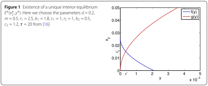
b1 , 0) and a

unique interior equilibrium E∗(x∗₂,y∗) (see Fig.1),which satisﬁes

x2=r1e

–dτ

b1 –

c1 b1y

m_≡_f₍_y_),

x2=r2

c2y

(1–m)₊b2 c2y

(2–m)_≡_g₍_y_).

(3)

Figure 1Existence of a unique interior equilibrium E∗(x∗₂,y∗). Here we choose the parametersd= 0.2, m= 0.5,r1= 2.5,b1= 1.8,c1= 1,r2= 1,b2= 0.5, c2= 1.2,τ= 20 from [16]

It is easy to see that the solutions (x2(t),y(t)) of system (1.4) with the initial conditions (1.5) exist for allt≥0 and are unique.

By the analysis of the characteristic equations and the iterative schemes coupled with the comparison principle, the dynamical properties of system (1.4) were established in [16]. That is, when (1 –m)2_r2_{> 2}_mr1_{, the interior equilibrium is locally asymptotically stable}

and globally attractive when the following inequality holds:

mr1e–dτ(r2+b2M) <r2r1e–dτ–c1Mm, (1.7)

whereM= (c2r1e–dτ

b1r2 ) 1 1–m_.

However, numerical simulations suggest that the unique interior equilibriumE∗of sys-tem (1.4) is always globally stable when it exists. Hence the authors in [16] raise two worthy problems: (i) Under some weaker conditions, or even without preconditions, whether sys-tem (1.4) has a unique interior equilibrium, which is globally stable. (ii) In more general situations, whether the mutual interference (0 <m< 1) can make the endangered species become globally stable.

The object of this study is to show that the interior equilibrium of system (1.4) is al-ways globally asymptotically stable as long as it exists and to give straightforward positive answers to the questions above.

2 Main result

In this section, by constructing suitable Lyapunov functionals for delay diﬀerential equa-tions system (1.4), we establish the global stability of the interior equilibrium when it exists for anyτ≥0.

Lemma 1 For any positive constants w and m where0 <m≤1,the following two inequal-ities hold:

1 –w1–m1 –wm≥0, (2.1)

1 –w2–m1 –wm≥0. (2.2)

Proof Letf1(w) = (1 –w1–m_{)(1 –}_wm_{) = 1 –}_wm_–_w1–m₊_w_{, then}

f₁(w) = –mwm–1– (1 –m)w–m+ 1 = – m

w1–m –

(4)

When 0 <w≤1, we havef₁(w) < 0. Whenw> 1, we havef₁(w) > 0. Thus, it has

Theorem 2.1 The interior equilibrium E∗(x∗₂,y∗)of system(1.4)is globally asymptotically stable for any delayτ≥0.

Proof Deﬁne the global Lyapunov functional forE∗,

U(t) =V1(t) +r1e–dτx∗2·V+(t) +

(5)

= –x2(t–τ)

Now, the time derivative ofU(t) computed along solutions of system (1.4) is

dU

By factoring the last two terms, we have

(6)

From Lemma1, for 0 <m< 1, we know that

1 –

y∗

y

2–m

1 –

y∗

y m

≥0, (2.7)

1 –

y∗

y

1–m

1 –

y∗

y m

≥0. (2.8)

Further, since the functionh(z) =z(t) – 1 –lnz(t) is always nonnegative for any function

z(t) > 0, andh(z) = 0 if and only ifz(t) = 1, we know that

x2(t–τ)

x2 – 1 –ln

x2(t–τ)

x2 ≥0. (2.9)

It follows that the positive-deﬁnite functionalU(t) has non-positive derivative_dtdU(t). Let Mbe the largest invariant subset of{(x2(t),y(t))| dU_dt = 0}. Since dU_dt equals zero if and

only ifx2(t) =x∗₂=x2(t–τ),y(t) =y∗, we see thatMis the singleton{E∗}. By the LaSalle invariance principle [7], every solution of system (1.4) tends to the interior equilibrium

E∗, which is globally asymptotically stable.

The proof is completed.

Remark The type of Lyapunov functionV1was ﬁrst used for the Lotka–Volterra system, and then it was successfully applied to epidemiological models by Korobeinikov [13,14]. Furthermore, McCluskey [17,18] extended it as the Lyapunov function of formV+for

some delay diﬀerential equations models.

3 Numerical simulations and conclusions

Here we perform numerical simulations to show that parametersmandτhave no eﬀects on the stability of the interior equilibriumE∗(x∗2,y∗) of system (1.4). Parameters values are

from [16] except formandτas follows:

d= 0.2, r1= 2.5, b1= 1.8, c1= 1,

r2= 1, b2= 0.5, c2= 1.2.

(3.1)

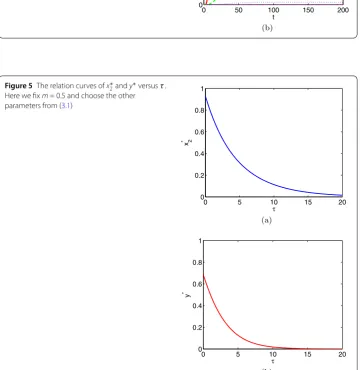
First, we fixτ= 2.5 and varym= 0.1, 0.3, 0.7, 0.9, which correspond to four values ofE∗= (0.346676, 0.320008), (0.444703, 0.328168), (0.62698, 0.258366), (0.741398, 0.150437). Fig-ure 2shows that all solutions tend toE∗. We can see that the value ofx∗₂ increases as the increase of m(see Fig.3(a)), but the value ofy∗ increases first and then decreases as the increase of m (see Fig. 3(b)). Second, we fix m= 0.5 and vary τ = 1, 5, 10, 20, which correspond to four values of E∗ = (0.742163, 0.505426), (0.313992, 0.125679), (0.113186, 0.0181181), (0.0152641, 0.000335395). Figure4also reveals that all solutions tend toE∗. And we found that the values of bothx∗₂andy∗decrease with the increase ofτ

(see Fig.5). In conclusion, bothmandτcan change the value ofE∗, but they cannot aﬀect the stability ofE∗.

(7)

Figure 2All solutions converge to the interior equilibriumE∗for diﬀerentm. Here we ﬁxτ= 2.5 and choose the other parameters from (3.1) with the initial condition (x2(0),y(0)) = (0.01, 0.001)

Figure 3The relation curves ofx2∗andy∗versusm. Here we ﬁxτ= 2.5 and choose the other

(8)

Figure 4All solutions converge to the interior equilibriumE∗for diﬀerentτ. Here we ﬁxm= 0.5 and choose the other parameters from (3.1) with the initial condition (x2(0),y(0)) = (0.01, 0.001)

(9)

(1.4) always exists and is globally asymptotically stable. This essentially improves the pre-vious stability results in [16]. On the other hand, whenτ= 0, system (1.4) will be simplified to the ordinary differential system. Theorem2.1indicates that mature period delay of prey does not affect the global asymptotic properties of the model.

In the special case ofm= 1 (that is, no mutual interference), system (1.4) has a positive equilibrium if and only if

r2 c2 <

r1e–dτ

b1 . (3.2)

By using the same Lyapunov functional, it is easy to see that the positive equilibrium is globally asymptotically stable when it exists. When we introduce mutual interference (0 <m< 1), system (1.4) always has a positive equilibrium. That is, we do not need the condition (3.2) to ensure the existence of positive equilibrium for 0 <m< 1. It means that the mutual interference (0 <m< 1) helps the endangered predators survive under any maturation time delay of preys.

We would like to point out that the Lyapunov approach in this study comes from the gen-eralization of our previous work in Huang et al. [10,11]. Here we applied the technology of constructing Lyapunov functionals to the delayed predator–prey model with mutual interference, and it can also be applied to some classes of systems similar to system (1.4).

Funding

This work was partially supported by the National Natural Science Foundation of China (Grant No. 11571326).

Competing interests

The authors declare that they have no competing interests.

Authors’ contributions

The authors contributed equally to the writing of this paper. The authors read and approved the ﬁnal manuscript.

Author details

1_{School of Mathematics and Physics, China University of Geosciences, Wuhan, China.}2_{School of Mathematics and} Statistics, Central China Normal University, Wuhan, China.

Publisher’s Note

Springer Nature remains neutral with regard to jurisdictional claims in published maps and institutional aﬃliations.

Received: 27 May 2018 Accepted: 17 August 2018 References

1. Aiello, W.G., Freedman, H.I.: A time-delay model of single-species growth with stage structure. Math. Biosci.101, 139–153 (1990)

2. Barclay, H.J., Van den Driessche, P.: A model for a species with two life history stages and added mortality. Ecol. Model.

11, 157–166 (1980)

3. Burnett, T.: Eﬀects of natural temperatures on oviposition of various numbers of an insect parasite (Hymenoptera, Chalcididae, Tenthredinidae). Ann. Entomol. Soc. Am.49, 55–59 (1956)

4. Freedman, H.I.: Graphical stability, enrichment, and pest control by a natural enemy. Math. Biosci.31, 207–225 (1976) 5. Freedman, H.I.: Stability analysis of a predator–prey system with mutual interference and density-dependent death

rates. Bull. Math. Biol.41, 67–78 (1979)

6. Freedman, H.I., Rao, V.S.: The trade-oﬀ between mutual interference and time lags in predator–prey systems. Bull. Math. Biol.45, 991–1004 (1983)

7. Hale, J., Verduyn Lunel, S.M.: Introduction to Functional Diﬀerential Equations, vol. 9. Applied Mathematical Science, New York (1993)

8. Hassell, M.P.: Mutual interference between searching insect parasites. J. Anim. Ecol.40, 473–486 (1971)

9. Hassell, M.P., Varley, G.C.: New inductive population model for insect parasites and its bearing on biological control. Nature223, 1133–1137 (1969)

10. Huang, G., Liu, A., Fory´s, U.: Global stability analysis of some nonlinear delay diﬀerential equations in population dynamics. J. Nonlinear Sci.26, 27–41 (2016)

(10)

12. Jiang, X., She, Z., Feng, Z., Zheng, X.: Bifurcation analysis of a predator–prey system with ratio-dependent functional response. Int. J. Bifurc. Chaos27, Article ID 1750222 (2017)

13. Korobeinikov, A., Maini, P.K.: A Lyapunov function and global properties for SIR and SEIR epidemiological models with nonlinear incidence. Math. Biosci. Eng.1, 57–60 (2004)

14. Korobeinikov, A., Wake, G.C.: Lyapunov functions and global stability for SIR, SIRS and SIS epidemiological models. Appl. Math. Lett.15, 955–961 (2002)

15. Li, H., She, Z.: Uniqueness of periodic solutions of a nonautonomous density-dependent predator–prey system. J. Math. Anal. Appl.422, 886–905 (2015)

16. Li, Z., Han, M., Chen, F.: Global stability of a predator–prey system with stage structure and mutual interference. Discrete Contin. Dyn. Syst., Ser. B19, 173–187 (2014)

17. McCluskey, C.C.: Global stability for an SEIR epidemiological model with varying infectivity and inﬁnite delay. Math. Biosci. Eng.6, 603–610 (2009)

18. McCluskey, C.C.: Complete global stability for an SIR epidemic model with delay—distributed or discrete. Nonlinear Anal., Real World Appl.11, 55–59 (2010)