R E S E A R C H
Open Access
Serial distributed detection for wireless
sensor networks with sensor failure
Junhai Luo
*and Zuoting Liu
Abstract
We study serial distributed detection and fusion over noisy channels in wireless sensor networks (WSNs) with bathtub-shaped failure (BSF) rate of the sensors in this paper. In the previous work, we applied BSF rate to parallel topology and derived the Extension Log-likelihood Ration Test (ELRT) rule. Although ELRT is superior to traditional fusion rule without considering failed sensors, the detection performance decreases noticeably in the presence of a large number of failed sensors. In this paper, we construct a serial topology based on the target radiation energy attenuation model, apply BSF rate to serial topology, and derive the corresponding fusion rule. Unlike the parallel fusion, where the local sensors send their decisions to the Global Fusion Center (GFC) in the region of interest (ROI) directly, sensors in the serial topology transmit local decisions through multi-hop, short-range communications. At the same time, we extend ELRT to noisy channels. Finally, simulation results prove the effectiveness of the proposed fusion rules.
Keywords: Serial distributed detection, bathtub-shaped failure rate, failed sensors
1 Introduction
WSNs have attracted many researchers in various disci-plines due to their flexibility, robustness, mobility, and cost-effectiveness. A major application of WSNs is tar-get detection. WSN typically consists of a vast number of small, inexpensive, and low-powered sensors, which are deployed in the ROI to obtain and preprocess the received observation. The GFC is making a final decision about whether the target is present or not. There are two popular detection methods: centralized detection and dis-tributed detection. In the centralized detection, the local sensor sends the received observation to the GFC directly without any processing. In the distributed detection, each sensor quantifies its observation into a local decision (“0” or “1”) and sends it to the GFC. Although centralized detection achieves the highest performance, it is at the cost of more bandwidth and communication energy to obtain real-time results. Thus, the distributed detection is often preferable in these situations.
Distributed target detection has been extensively stud-ied in many kinds of literature. In [1, 2], each sensor made a local decision by conducting likelihood ratio test
*Correspondence: [email protected]
School of Electronic Engineering, University of Electronic Science and Technology of China, No. 2006, Xiyuan Ave, West Hi-Tech Zone, 611731 Chengdu, China
and sent the local decision to the GFC to perform global log-likelihood ratio test, and then the GFC made a final decision. In [3], a uniformly most powerful (UMP) detec-tor based on likelihood ratio test was developed, and an elegant test for target presence or absence was also derived. Typically, the performance of local sensors is hard to calculate. Therefore, in [4], a suboptimal fusion rule requiring less prior information was proposed, which we refer to as the counting rule (CR). CR employed the total number of decisions transmitted from local sen-sors for hypothesis testing at the GFC. In [5], CR was extended to the case where the total number of sensors was uncertain. Authors in [6–9] took into account imper-fect communication channels between the sensors and the GFC, such as additive white Gaussian noise (AWGN) channels and fading channels. In [6], noisy communica-tion links were considered and a Bayesian framework for distributed detection was presented, where noisy links were modeled as binary symmetric channels (BSC). In [7], distributed detection fusion in hierarchical WSNs was investigated in the presence of fading and noise, two fusion rules were derived accordingly, one utilized the complete fading channel state information (CSI), the other utilized the channel envelope statistics (CS). For resource-constrained sensor networks, a fusion rule using CSI was more preferable. Typically, local sensors communicated
with the GFC directly. In [10], authors considered the case where local decisions need to be relayed through the multi-hop transmission to reach the GFC and also took fading into account. In [11], based on various decisions from local sensors, a decision rule was derived in the case of unknown probability distributions. In [12, 13], deci-sion fudeci-sion rules with unknown detection probability were investigated. Clustering-based decision fusion algorithms and fusion rules for distributed target detection in WSNs were studied in [14–16].
The structure of the WSNs can be classified into three categories: parallel topology, serial topology, and tree topology. Most researchers focus on parallel distributed detection. However, sensors are usually powered by a bat-tery, so the energy and the communication range are limited. When sensors are far away from the GFC, the power consumption increases dramatically and the life-time of the WSN has shortened accordingly. In [17, 18], serial distributed detection was investigated, where local decisions are transmitted to the GFC through short-range and multi-hop communication. The channel between two adjacent sensors was modeled as BSC. However, authors in [17] assumed the received energy emitted by the tar-get at the local sensors was a deterministic value. In this case, the detection performances of the local sensors were similar.
The most common practice of traditional fusion rules, such as CR and Chair-Varshney fusion rules, is to employ all sensors in the ROI to derive a final decision. How-ever, the signal emitted by the target often decays as the distance from the target increases. Sensors far away from the target make little contribution to the final decision at the GFC or are more likely to make a false judgment in the presence of background noise. In this paper, we sim-ply employ sensors around the target to make the final decision.
We propose a new serial topology reconstruction method, where decisions are transmitted from sensors with lower credibility to sensors with higher credibil-ity. Assuming the transmission channels were ideal, we applied a BSF rate of the sensor into the parallel struc-ture and proposed ELRT in [19]. In this paper, we solve the problem when there are failed sensors in the serial structure and propose the corresponding fusion rule over noisy channels which we call serial rule (SR). In order to demonstrate the more stable detection performance of the serial structure, we also extend ELRT to noisy chan-nels and derive the corresponding fusion rule in the same scenario which we call parallel rule (PR).
The remainder of this paper is organized as follows. In Section 2, the BSF rate of the sensor is described. In Section 3, a sensor deployment model is described. In Section 4, a detection system model is described. In Section 5, the fusion rules of the serial and parallel
structure are derived. In Section 5, the performance of the proposed fusion rules is provided through simulation. In Section 6, conclusions are drawn.
2 BSF rate
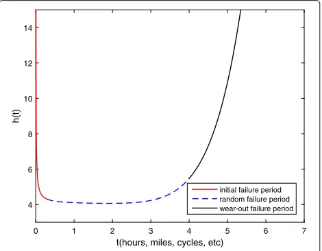
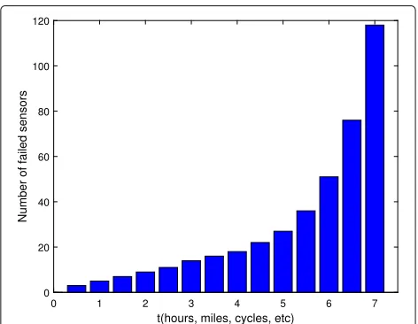
One can characterize a lifetime distribution through three functions: reliability function, failure rate function, and mean residual life [20]. The lifetime typically means the time the product can operate regularly before it fails and can be measured in hours, miles, cycles, etc. In our orig-inal research work [19], we used failure rate function to characterize the lifetime distribution of electronic compo-nents. The failure rate function is shown in Fig. 1, which we call BSF. We can see that the failure rate function has a bathtub shape and can be visually subdivided into three stages: initial failure period, random failure period, and wear-out failure period. The initial failure period starts at zero and decreases noticeably due to early failures caused by design faults or initial implementation problems. The random failure period is relatively flat (approximately con-stant), which is denoted as the “useful life” phase. The failure is noticeably increasing due to material fatigue or component aging during wear-out failure period [21]. We also gave the modified failure rate functionr(t)as follows in [19]
r(t)=ab(at)b−1+ a
b
(at)1b−1+h0, t,a,h0≥0,b>1 (1)
whereaandbare related with life data of the products and
h0is a worthy constant adding to the failure rate function. Thus, sensors in this paper can be classified into four categories
• Normal sensors, sensors that can detect and transmit
decision reliably
• Partially disable sensors, sensors that are still operable, but have poor detection capability
• Inoperable sensors, sensors which no longer function
at all
• Failed sensors, the group of sensors consisting of the
combination of the partially disable and the inoperable sensors
LetNdenote the initial number of the sensors,Mbe the number of the sensors excluding the inoperable sensors,n
be the number of normal sensors, andmbe the number of failed sensors at timet, respectively. We can easily get that
n=N−m.mcan be written as
m=ceil
t
0 r(t)dt
(2)
where ceil(·)denotes the ceiling function.
Irrespective of the inoperable sensors at time t, the remaining sensor is either a normal sensor or a partially disable sensor.Ri=1 which represents sensorsiis a
nor-mal sensor, and Ri=0 which represents sensor si is a
partially disable sensor. The probability that sensorsiis a
partially disable sensor is given as follows
pi =Pr(Ri=0)
=Pr(sensor siis a partially disable sensor)
= s M
= M−n M
= M−N+m
M (0≤s≤m, 0<M≤N)
(3)
wheresis the number of the partially disable sensors at timet, it is easy to note thatpi is constant at timetand
Pr(Ri=1)=1−pi. We usepwhich denotes Pr(Ri=0)
in the latter sections.
3 Sensor deployment model
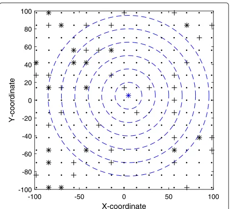
A sensor deployment example in the presence of failed sensors is shown in Fig. 2. N sensors follow the grid deployment, and a target is deployed randomly in the ROI. The target and different types of sensors are labeled by dif-ferent symbols. The received signal power emitted by the targetmi,i=1, 2,. . .,Nof sensorsidecays as the distance from the target increases. An isotropic attenuation power model adopted in this paper is defined as follows
m2i = P0D γ 0
Dγi (4)
where P0is the signal power from the target at a refer-ence distanceD0andDirepresents the Euclidean distance between the target and sensorsi. The signal attenuation exponentγ ranges from 2 to 3.
Signal power versus distance from the target is shown in Fig. 3. We can see that target radiation energy decays rapidly as the distance from the target increases. Sensors
Fig. 2A deployment example in the presence of failed sensors. Area of the ROI:A2;black dot: the normal sensors;black star: the inoperable sensors;black +: the partially disable sensors; andblue star: the target
far away from the target are prone to make wrong deci-sions influenced by background noise. Authors in [14] establish the precursor-successor relationship among the clusters based on tree topology. The cluster the target located in serves as the root cluster and the other clusters serve as the branch or leaf clusters, in this way, the root cluster can achieve the highest detection performance. Authors in [22] study a binary tree topology, where the sensor nearest the target serves as the root. Authors in [23, 24] think there are several “target spots” in the ROI where the target often appears, then analyze the area cen-tered at the “target spot” and propose a target detection
Fig. 3Signal power versus distance from target, where
algorithm based on a probabilistic decision model. So, it is reasonable for us to investigate the area centered at the target in this paper.
The radiation energy of the target can be assumed as a series of concentric circles centered at the target. In this paper, we set the interval between two adjacent circles identical. Sensors lying in the same circular ring possess similar signal-to-noise ratio (SNR) and decision credibil-ity, and the circular ring interval is 10. Due to the fast attenuation of the target radiation energy, we consider the circular area of the radius of 40 centered at the tar-get in this paper. Firstly, sensors in the same circular ring form a serial fragment, then all fragments form the whole serial topology from the outside to the inside. We can see that decisions are transmitted from sensors with lower credibility to sensors with higher credibility in this serial structure, so the final decision at the last sensor of the serial structure possesses the highest credibility.
4 System model description
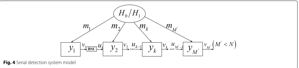
Figure 4 describes the serial detection system model. We leave out the inoperable sensors and form a new serial topology at timet. So the serial topology is dynamic. The wireless transmission channel between two adjacent sen-sors is modeled as BSC with transmission error probabil-itype. The observation of sensorsiunder each hypothesis is respectively given by
H1:yi=mi+ni ; i=1,. . .,M
H0:yi=ni ; i=1,. . .,M
M <N
(5)
H0andH1denote the absence and the presence of the target to be detected respectively.Mis the number of sen-sors in the serial topology at timet.yiis the signal received
by sensorsi, andni is the noise observed by sensorsi. In
this paper, we assume that noises at the local sensors are independent identically distributed (i.i.d.) and follow the standard Gaussian distribution, i.e,ni∼N(0, 1).
In Fig. 4,videnotes the decision made by sensorsi, and
uidenotes the bit received by sensorsi+1which may differ fromvi. Sensors1tosM cooperatively determine whether the target is present or not in the ROI. SensorsM is the fusion center (FC) of the serial structure at timet. Because
we apply BSF to the serial structure, sM may be a par-tially disable sensor. IfsM is a partially disable sensor, the final decision is not reliable. In this paper, we let sensor
sM transmits its observation to the GFC, then the GFC replaces sensorsMand serves as the FC of the serial struc-ture. In this way, theMth sensor of the serial structure in Fig. 4 is actually the GFC at timet.
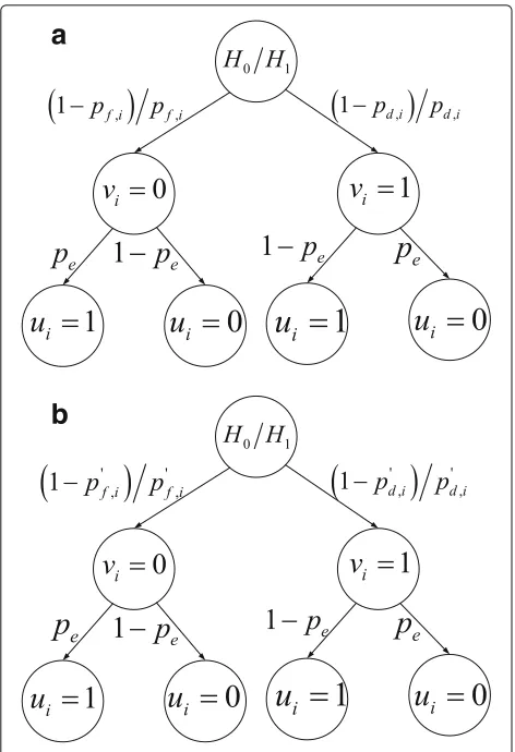
In Fig. 5, a and b give the local decision-making and transmission process at sensor si under the situa-tion ofRi=1 andRi=0, respectively. UnderH0, when Ri=1, sensor si makes a correct decision with
proba-bility 1−pf,i, and an error decision with probabilitypf,i, while whenRi=0, sensorsimakes a correct decision with
probability 1−pf,i, and an error decision with
probabil-itypf,i. During the decision transmission process, the bit
ui received by sensorsi+1may differ from the decisionvi
made by sensorsidue to the noisy channel. The situation
underH1is similar to that underH0, except that the detec-tion performance is denoted by pd,i and p
d,i. Normally, pd,i≤pd,i,pf,i≤pf,i.
5 SR and PR
5.1 SR
Letp(yi|H1)andp(yi|H0)represent the conditional prob-ability density function of the observationyiat sensorsi
underH1andH0, respectively. Except that sensors1makes the local decision simply according to its observationy1, the other sensors make decision according to their obser-vations and the bit transmitted from the previous sensor. For example, sensors1makes a decisionv1according to its observationy1, while sensors2makes a decision accord-ing to its observationy2and the bitu1transmitted from sensors1, whereu1may be different fromv1. For sensor si
1<i≤M <N
, the decision-making process is sim-ilar to sensors2. The likelihood ratio test at sensors1can be expressed as
0(y1)= p(y1|H1) p(y1|H0)
H1
≷
H0
τ (6)
Given the local thresholdτ and according to Neyman-Pearson criterion, the detection probability and false
Fig. 5Model of serial distributed detection under noisy channel. aandbdescribe the situation ofRi=1 andRi=0, respectively
alarm probability at sensors1can be evaluated easily. The likelihood ratio test at sensorsi
1<i≤M <N
can be expressed as
0(yi)=
p(yi,ui−1|H1) p(yi,ui−1|H0)
H1
≷
H0
τ (7)
Because of the independence between yi and ui−1, 0(yi)can be further expressed as follows
0(yi)=
p(yi|H1)·p(ui−1|H1) p(yi|H0)·p(ui−1|H0)
(8)
Let us discuss p(ui−1|H1) firstly. Due to BSC, the received bitui−1at sensorsidepends on the decisionvi−1 made at sensorsi−1, thus we can get
p(ui−1|H1) =vi−1p(ui−1,vi−1|H1)
=p(ui−1,vi−1=1|H1)
+p(ui−1,vi−1=0|H1)
=p(ui−1|vi−1=1,H1)p(vi−1=1|H1)
+p(ui−1|vi−1=0,H1)p(vi−1=0|H1)
=p(ui−1|vi−1=1)p(vi−1=1|H1)
+p(ui−1|vi−1=0)p(vi−1=0|H1) (9)
In the above equation, we use the Markov property that ui−1 is only dependent on vi−1. This property will be exploited in the following derivations. Note that the decisionvi−1at sensorsi−1depends on whethersi−1is a partially disable sensor or not. Furthermore, we can easily get
ai−1 =p(vi−1=1|H1)
=Ri−1p(vi−1=1,Ri−1|H1)
=p(vi−1=1,Ri−1=1|H1)
+p(vi−1=1,Ri−1=0|H1)
=p(vi−1=1|Ri−1=1,H1)p(Ri−1=1|H1)
+p(vi−1=1|Ri−1=0,H1)p(Ri−1=0|H1)
=(1−p)pd,i−1+pp d,i−1
(10)
and
bi−1 =p(vi−1=0|H1)
=Ri−1p(vi−1=0,Ri−1|H1)
=p(vi−1=0,Ri−1=1|H1)
+p(vi−1=0,Ri−1=0|H1)
=p(vi−1=0|Ri−1=1,H1)p(Ri−1=1|H1)
+p(vi−1=0|Ri−1=0,H1)p(Ri−1=0|H1)
=(1−p)1−pd,i−1 +p
1−pd,i−1
(11)
whenui−1=1,
αi−1 =vi−1p(ui−1,vi−1|H1)
|(ui−1=1)
=(1−pe)ai−1+pebi−1
(12)
Similarly, whenui−1=0,
βi−1 =vi−1p(ui−1,vi−1|H1)
|(ui−1=0)
=peai−1+(1−pe)bi−1
(13)
So,p(ui−1|H1)can be expressed as
p(ui−1|H1)=(αi−1)ui−1·(βi−1)1−ui−1 (14)
Next, let us discussp(ui−1|H0) p(ui−1|H0) =vi−1p(ui−1,vi−1|H0)
=p(ui−1,vi−1=1|H0)
+p(ui−1,vi−1=0|H0)
=p(ui−1|vi−1=1,H0)p(vi−1=1|H0)
+p(ui−1|vi−1=0,H0)p(vi−1=0|H0)
=p(ui−1|vi−1=1)p(vi−1=1|H0)
We can get
After a series of derivation, the likelihood ratio test at sensorsiin Eq. (7) can be formulated as
0(yi)= p(yi|H1)
Now, the decision rule of sensorsican be given by ⎧
Furthermore, the decision fusion rule in Eq. (22) can be transformed into
We should note that (yi)is another metric we defined
and is different from0(yi), where
τi,1=τ·αγii−−11,τi,0=τ·ηβii−−11 (24) The corresponding log-likelihood ratio form of Eq. (23) can be formulated as
The false alarm probability and the detection probability at sensorsiare evaluated as follows
pf,i LetPd andPf represent the global detection probability
and false probability, respectively, we note thatPd=pd,M
andPf =pf,M. Givenτ,pf,1andpd,1at sensors1can be easily derived according to Eq. (6).
pf,1=
whereQ(·)is the complementary distribution function of the standard Gaussian, i.e,
To demonstrate the better detection performance of SR, we extend ELRT [19] to noisy channels and propose PR in the same scenario. In the parallel structure, the local sen-sorsimakes a local decisionvpi(1≤i≤M)and transmits
it to the GFC in the ROI. We denoteupias the bit received
with transmission error probability pe. Furthermore, we
Due to the mutual independence among the received bits, the fusion rule at the GFC is given as follows
1= p
According to SR,1can be further represented as
1=M
whereT denotes the detection threshold at the GFC,pe
and p are given in the previous section. pp,di and p p,di
denote the local detection probability when sensorsiis a
normal sensor and a partially disable sensor, respectively. Similarly,pp,fi andp
p,fi denote the local false probability.
Given the local threshold, according to Neyman-Pearson criterion, we can get the local detection probability and false probability easily. The log-likelihood ratio form is given as follows
The final fusion rule at the GFC is as follows
1
global detection probability and false probability of the parallel structure respectively.Ppd andPpf can be
evalu-ated as
We use the Matlab simulator to evaluate the performance of the proposed fusion rules in this paper, and 104Monte Carlo runs are used in each simulation. The objective is to demonstrate that serial structure has more stable detection performance than the parallel structure in the presence of a vast number of failed sensors. In [19], we studied the parallel distributed detection applying BSF rate of the sensor over ideal channels and proposed ELRT rule. Simulations demonstrated that ELRT outperformed Chair-Varshney rule in the presence of failed sensors. In this paper, we apply BSF to the serial structure over noisy channels and also extend ELRT to noisy channels, because sensors far away from the target make little contribu-tions to the final decision at the GFC and are more likely to make wrong decisions in the presence of background noise. Thus, we consider sensors within the circular area centered at the target in this paper, the deployment in the presence of failed sensors is presented in Fig. 2. The fusion rules of the serial and parallel are given in the previous sections.
In Fig. 6, according to Eq. (2), the number of failed sensors including the partially disable sensors and the inoperable sensors is plotted as a function of
t(hours, miles, cycles, etc)and the corresponding parame-ters are given at the bottom. We can see that the number of failed sensors during the initial failure period is negli-gible, such ast=0.5. The number increases slowly at the low time, while the number grows noticeably after time 5. The curve of the number of failed sensors over time also reflects the feature of BSF.
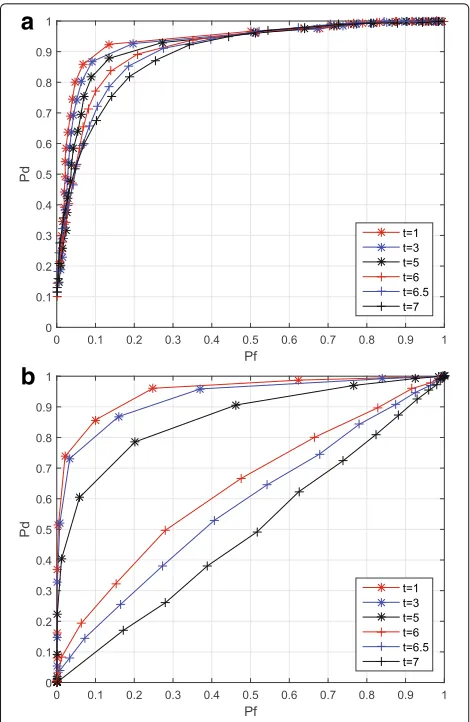
We leave out the inoperable sensors at each time, the partially disable sensors are selected from the remaining sensors randomly. In Fig. 7, a and b show the receiver
Fig. 7The ROC curses of SR and PR at a different time:γ=2,
A=200 m,D0=1 m,N=220,P0=180,N−mM=13,p
d,i= pd,i
5 ,
pf,i=0.5,a=0.25,b=8, andh0=4.a,bcorrespond to the ROC curses of SR and PR, respectively
operating characteristic (ROC) curves for SR and PR, respectively. The simulation parameters for these two rules are set to be identical and given at the bottom. We uset=1,t=3,t=5,t=6,t=6.5, andt=7 to conduct the experiment and choosepd,i=pd,i/5 andpf,i=0.5 for the partially disable sensor due to their poor performance. In Fig. 7a, we see that the performance of SR decreases slightly all the time. In Fig. 7b, we observe that the perfor-mance of PR decreases slowly before time 5 and noticeably after time 5. For PR, sensors in the parallel structure make local decisions and transmit the decisions to the GFC directly. At the low time, a small number of failed sensors have a negative but not big effect on the system perfor-mance. Meanwhile, at the high time, a large number of failed sensors have a major negative effect on the system performance. For SR, each sensor in the serial structure makes a decision according to the bit transmitted from the
previous sensor and the state (partially disable or normal) of the previous sensor, and due to this cooperative detec-tion, SR has more stable detection performance even in the presence of a large number of failed sensors at high time. We should note that BSF influences the detection performances of both serial and parallel structures.
The above analysis demonstrates the effectiveness of SR. In order to investigate the impact of SNR on the detec-tion performance of SR, Fig. 8 shows the global detecdetec-tion probabilityPdversus SNR over time. SNR is defined as the
ratio of source energy to the standard deviation of noise, namely SNR=10 log
S N
, where S=P0,N=1 in this paper. We can see that higher SNR leads to higher global detection probability. Comparing the curves at a different time, it is easy to note that when SNR is fixed, detection probability at a lower time is superior to higher time, and this is in accordance with the results of ROC.
7 Conclusions
This paper investigates distributed decision fusion of serial structure in the presence of failed sensors over noisy channels. Previous literature focus on serial structure usu-ally assumes the signal received by the local sensor is identical. While in this paper we construct a serial topol-ogy based on isotropic attenuation power model, the local decision in this topology is transmitted from sensors with lower credibility to sensors with higher credibility. We also derive the corresponding fusion rule. For comparison, we extend ELRT to noisy channels in the same scenario. Sim-ulations show that serial is more robust than parallel in the presence of a large number of failed sensor over noisy channels. The deployment we considered in this paper is relatively ideal, we will study different deployment in the future.
Acknowledgements
This work was supported in part by the Overseas Academic Training Funds, University of Electronic Science and Technology of China (OATF, UESTC) (Grant No. 201506075013), and the Program for Science and Technology Support in Sichuan Province (Grant nos. 2014GZ0100 and 2016GZ0088).
Authors’ contributions
JL conceived of and designed the research. JL and ZL performed the experiments and analyzed the result. JL and ZL wrote the paper. Both authors read and approved the final manuscript.
Competing interests
The authors declare that they have no competing interests.
Publisher’s Note
Springer Nature remains neutral with regard to jurisdictional claims in published maps and institutional affiliations.
Received: 20 January 2016 Accepted: 30 June 2017
References
1. Z Chair, PK Varshney, Optimal data fusion in multiple sensor detection systems. IEEE Trans. Aerosp. Electron. Syst.22(1), 98–101 (1986) 2. IY Hoballah, PK Varshney, Distributed Bayesian signal detection. IEEE
Trans. Inf. Theory.35(5), 995-1000 (1989)
3. T-L Chin, YH Hu, Optimal Detector Based on Data Fusion for Wireless Sensor Networks, Global Telecommunications Conference (GLOBECOM 2011). IEEE, Kathmandu, Nepal.6613(1), 1–5 (2011)
4. R Niu, PK Varshney, Q Cheng, Distributed detection in a large wireless sensor network. Inf. Fusion.7(4), 380–394 (2006)
5. R Niu, PK Varshney, Distributed Detection and Fusion in a Large Wireless Sensor Network of Random Size. EURASIP J. Wirel. Commun. Netw.
2005(4), 462–472 (2005)
6. Decentralized binary detection with noisy communication links. IEEE Trans. Aerosp. Electron. Syst.42(4), 1554–1563 (2006)
7. K Eritmen, M Keskinoz, Distributed decision fusion over fading channels in hierarchical wireless sensor networks. Wirel. Netw.20(5), 987–1002 (2014) 8. R Niu, B Chen, PK Varshney, Fusion of decisions transmitted over Rayleigh
fading channels in wireless sensor networks. IEEE Trans. Signal Process.
54(3), 1018–1027 (2006)
9. Y Xia, F Wang, W-S Deng, The decision fusion in the wireless network with possible transmission errors. Inf. Sci.199(15), 193–203 (2012)
10. Y Lin, B Chen, PK Varshney, Decision fusion rules in multi-hop wireless sensor networks. IEEE Trans. Aerosp. Electron. Syst.41(2), 475–488 (2005) 11. AM Aziz, A new multiple decisions fusion rule for targets detection in
multiple sensors distributed detection systems with data fusion. Inf. Fusion.18(1), 175–186 (2014)
12. J-Y Wu, C-W Wu, T-Y Wang, et al., Channel-aware decision fusion with unknown local sensor detection probability. IEEE Trans. Signal Process.
58(3), 1457–1463 (2010)
13. D Ciuonzo, PS Rossi, Decision fusion with unknown sensor detection probability. IEEE Signal Process. Lett.21(2), 208–212 (2014)
14. H Huang, L Chen, X Cao, et al., Weight-based clustering decision fusion algorithm for distributed target detection in wireless sensor networks. Int. J. Distrib. Sensor Netw.2013, 1–9 (2013)
15. G Ferrari, M Martalo, R Pagliari, Decentralized detection in clustered sensor networks. IEEE Trans. Aerosp. Electron. Syst.47(2), 959–973 (2011) 16. Q Tian, EJ Coyle, Optimal distributed detection in clustered wireless
sensor networks. IEEE Trans. Signal Process.55(7), 3892–3904 (2007) 17. L Yin, Y Wang, D-W Yue,Serial Distributed Detection Performance Analysis in
Wireless Sensor Networks Under Noisy Channel, Wireless Communications, Networking and Mobile Computing. (IEEE, Beijing, 2009), pp. 3092–3095 18. M Lucchi, M Chiani,Distributed Detection of Local Phenomena with Wireless
Sensor Networks, 2010 IEEE International Conference on Communications (ICC 2010). (IEEE, Cape Town), pp. 1–6
19. J Luo, T Li, Bathtub-shaped failure rate of sensors for distributed detection and fusion. Math. Probl. Eng.2014, 1–8 (2014)
20. CD Lai, M Xie, DNP Murthy, inAdvances in Reliability. Chapter 3. Bathtubshaped failure rate life distributions, vol. 20 of Handbook of Statistics. (2001), pp. 69–104
21. M Bebbington, C-D Lai, R Zitikis, Useful periods for lifetime distributions with bathtub shaped hazard rate functions. IEEE Transactions on Reliability.55, 245–251 (2006)
22. J Ni, J Mei,A Fusion Algorithm for Target Detection in Distributed Sensor Networks. Computational Intelligence and Communication Networks (CICN). (IEEE, Bhopal, 2014), pp. 349–353
23. T Wang, Z Peng, J Liang, et al.,Detecting Targets Based on a Realistic Detection and Decision Model in Wireless Sensor Networks. International Conference on Wireless Algorithms, Systems, and Applications WASA. (Springer, 2015), pp. 836–844