R E S E A R C H
Open Access
A fractional order model for obesity
epidemic in a non-constant population
In this paper, we propose a fractional order epidemic model for obesity contagion. The population size is assumed to be nonconstant, which is more realistic. The model considers vertical transmission of obesity and also obesity-related death rate. We give local stability analysis of the model. Finally, some numerical examples are presented.
MSC: 34A08; 92B99; 34D20; 37N25
Keywords: fractional differential equations; epidemic model; stability analysis; obesity
1 Introduction
Overweight and obesity are defined as abnormal and excessive fat accumulation that presents a risk to health []. Obesity is measured by using a number called body mass index (BMI) which is calculated by using the formula
BMI=W
H,
whereWis the weight of a person in kilograms andHis the height of a person in meters. If ≤BMI< , then the person is said to be overweight, and ifBMI≥, then the person is said to be obese.
Obesity is one of the major risk factors for many chronic, fatal diseases including cancer, diabetes mellitus and cardiovascular disorders. According to the World Health Organiza-tion, worldwide obesity has doubled since , and in , %of adults aged and over were obese [].
Although there are some other reasons (e.g. genetic reasons, endocrine disorders), the main reason for obesity is excessive food intake and lack of physical activity. These rea-sons are closely related to the life-styles of the individuals within a population. Therefore, obesity can be considered as socially contagious. In [] a detailed analysis of the obesity epidemic in the U.S. is given. Santonja et al. [] and Ejima et al. [] also considered obesity as an epidemic disease and gave mathematical models to explain the spread of obesity. In both of these models integer order differential equations are used and the total population size is assumed to be constant.
The epidemic models where the total population is assumed to be constant are classical models given for short-term epidemics. When the epidemic disease arises and vanishes in
a short time like influenza, this kind of models give realistic results. But in the case of long-term effective diseases like hepatitis, rabies, rubella and so on, limiting the population to be constant would be a very strong assumption that affects the realism of the model. In this paper, we propose a new mathematical model in which we assume that the population is nonconstant. What is more, with a particular choice of the natural death rate function in the model, it gives a classical logistic growth for the population.
We also consider the memory dependence on the obesity contagion. The memory ef-fect in the spread of obesity is discussed in detail in []. In recent years, it has frequently been observed in modeling memory-dependent processes of physical and life sciences that models based on fractional order derivatives provide better agreement between solutions and real data [–]. Therefore, it is reasonable to use fractional order models to under-stand the spread of obesity in a population. Also note that the fractional order model we give is a generalization of an integer order model, and if the order of the fractional model is one, it reduces to its integer order counterpart.
In this paper, we consider continuous fractional differential equation systems to under-stand the spread of obesity in a population. Discrete fractional systems are also being used to model some real life problems, and their stability results are given in recent years [, ]. Stability of the proposed model in this paper is examined using the method given by Matignon []. Some other stability results can be found in [–].
This paper is organized as follows. Section is devoted to the model construction. In this section we propose a new fractional order epidemic model including disease-dependent death rate within a nonconstant population size. We also consider the tendency to obesity at birth as a result of bad nutritional habits during pregnancy, by means of vertical trans-mission. In Section , a detailed local stability analysis for the model is given. Finally, in Section , we give some numerical examples to illustrate our results.
2 Mathematical model
We first give some basic definitions of fractional calculus.
Definition The fractional integral of orderμ> of a functionf :R+→Ris defined by
Here and elsewheredenotes the gamma function.
Fractional derivative has several different definitions []. In this paper we use the Ca-puto definition due to its advantages in applied problems. The CaCa-puto definition of frac-tional derivative allows us to use initial conditions of the classical form, avoiding solvability problems.
Definition Caputo fractional derivative of orderμ> of the functionf :R+→Ris defined by (if exists)
Dμf(t) =In–μDnf(t),
Figure 1 The schematic diagram of the model.
In our model, we assume that the total populationN(t) is partitioned into three classes
W(t),W(t),W(t) denoting normal weight, overweight and obese individuals at time t, respectively. For the model we study in this paper, we consider both horizontal and ver-tical transmission of the disease. We treat excess weight gain as an epidemic disease that spreads via social contact. We also take into account the fact that overweight babies may be born because of bad nutritional habits during the pregnancy periods. The parameters we use in our model are as follows:
p: probability of having an overweight baby;
b: natural birth rate;
d(·): natural death rate function (dependent on the total population); α: transmission rate of the disease by social contact;
β: rate at which an overweight individual moves to the obese class;
k,r: treatment rates for overweight and obese individual, respectively; θ: obesity-related (from the diseases that are caused by obesity) death rate.
We assume thatb,α,β,k,randθare all nonnegative constants. Let the natural death rate function be a continuous and nondecreasing function ofN. Also assume that there exists a positive constantMsuch thatd(M) =b.
The schematic diagram of our model can be seen in Figure . The system of fractional order nonlinear ordinary differential equations for the proposed model is given by:
DμW Equation () is in fact obtained by modifying the classical integer order model. Equation () includes a free parameterμthat may help the theoretical formulation of the solution fit better with the real data [–]. To the best of our knowledge, this model (also the integer order counterpart) is a new model for the obesity contagion.
Adding up the equations given in (), we have
DμN=b–d(N)N–θW. ()
Theorem There is a unique solution for the initial value problem given by()and the initial conditions
W() =W, W() =W, W() =W, ()
and the solution remains in R +.
Proof It is easy to see the existence and uniqueness of the solution of the initial value problem ()-() in (,∞). We will show that the domainR
on each hyperplane bounding the nonnegative orthant, the vector field points intoR +.
3 Equilibrium points and stability
For simplicity in calculations, we will consider the system
DμW= ( –p)bN+k(N–W–W) – only ifp= . The basic reproductive number of the given system is
R=
k+α–θ
(k+b)(β+r+b+θ). ()
Theorem The DFE of system() (if exists)is asymptotically stable if R< .
Proof The characteristic equation of system () is
f(λ) =d(M)M+λAλ+Bλ+C= , () where
A= –,
C=β(α+k–θ) – (k+b)(β+r+b+θ).
The DFE of system () is asymptotically stable if all of the roots of the characteristic equa-tion ()λi,i= , , , satisfy the following condition [, ]:
We now discuss the existence and stability of positive equilibrium. Positive equilibrium of system () isF= (W∗,W∗,N∗), where there exists positiveW∗, where
A,=
–(X+X)±
(X+X)– (X+X)
X=r+θ+β,
X= –b,
X=θβ.
The Jacobian matrixJ(F) evaluated at the endemic equilibrium is given by
J(F) =
Then the characteristic equation of the linearized system is in the form
aλ+aλ+aλ+a= ()
Corollary Let abe as given in().If a> ,then the positive equilibrium point of system ()is unstable.
Proof Using Descartes’ rule of signs, it is clear that ifa> then the characteristic equa-tion () has at least one positive root. So, the positive equilibrium F of system () is
unstable.
4 Numerical results
In this section we consider four sets of parameters to discuss different cases. We use the solution technique given in [] to evaluate the numerical solutions of the system forμ
Theorem ([]) Let · denote any convenient norm on Rn.Assume that f ∈C[R
,Rn],
where R= [(t,X) : ≤t≤a andX–X ≤b],f= (f,f, . . . ,fn)T,X= (x,x, . . . ,xn)T,and
letf(t,X) ≤S on R.Then there exists at least one solution for the system of FDEs given
by
DαX(t) =ft,X(t) ()
with the initial conditions
X() =X ()
on≤t≤β,whereβ=min(a, [bS(α+ )]α), <α< .
Theorem ([]) Consider the initial value problem given by()and()of orderα, <α< .Let
gv,X∗(v)=ft–tα–v(α+ )/α,Xt–tα–v(α+ )/α
and assume that the conditions of Theoremhold.Then a solution of()and()can be given by
X(t) =X∗tα/(α+ ),
where X∗(v)is a solution of the system of integer order differential equations
d(X∗(v))
dv =g
v,X∗(v)
with the initial conditions
X∗() =X.
We use the corresponding parameter values given in Table for each case. Population data for Turkey are used in numerical simulations. Some of the values given in Table are taken from real data. A linear, population-dependent death rate function is evaluated
Table 1 Parameter values for Case 1-4
Case 1 Case 2 Case 3 Case 4
p= 0.2 0.2 0.2 0.0
[22]b= 0.017 0.017 0.017 0.017
M= 243.926 243.926 243.926 243.926
α= 0.3 0.3 0.3 0.01
β= 0.2 0.2 0.2 0.2
k= 0.005 0.05 0.1 0.008
r= 0.002 0.02 0.2 0.2
[23]θ= 0.009 0.009 0.009 0.009
N(0) = 76 76 76 76
[24]S(0) = 26.676 26.676 26.676 26.676
using the data in [] asd(N) = (. + .N)–.Mvalue is calculated using the functiondand the valueb.
This linear death rate function lets the total populationNhave logistic growth. For the exact solution of a fractional logistic equation, [] used the Carleman embedding tech-nique, but there is a controversy between the results of West and Area et al. []. However, in this paper we use a totally different technique [] to find the solution of the system in-cluding the logistic equation.
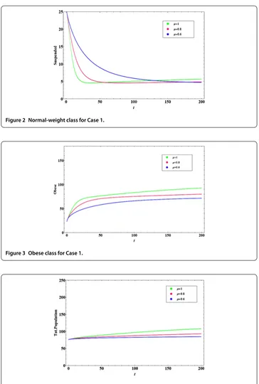
Case : System () has a positive fixed pointF,∗ = (., ., .). The roots of the characteristic polynomial of the given system atF,∗ are
λ= –.,
λ= –. + .i,
λ= –. – .i.
For allμ∈(, ],F,∗ is asymptotically stable.
Case : In Case , we use the same parameter values with the previous case except for
kandrwhich are the control parameters. These parameters can be adjusted according to the disease prevention and control strategies. Using the newkandrparameter values, the positive fixed point of system () can be evaluated asF,∗ = (., ., .). Askandrincrease,I∗decreases. The roots of the characteristic polynomial of the given system atF,∗ are
λ= –.,
λ= –. – .i,
λ= –. – .i.
So, even for this case, the positive equilibrium point is asymptotically stable for allμ∈
(, ].
Case : In this case, we use greaterkandrvalues compared to the previous cases. The positive fixed point in this case isF,∗ = (., ., .). The roots of the char-acteristic polynomial atF,∗ are
λ= –.,
λ= . + .i,
λ= . – .i.
Forμ= ,F,∗ is unstable. Using (), it can be shown that forμvalue less than .,
F,∗ is asymptotically stable.
Case : We now consider the case where vertical transmission of the disease does not exist, i.e.p= . The value ofpis also related to the disease control and prevention strate-gies. For this case, the DFE exists. ForF∗= (., , .), the basic reproductive numberR= ., which states thatF∗is asymptotically stable for allμ∈(, ].
Figure 2 Normal-weight class for Case 1.
Figure 3 Obese class for Case 1.
Figure 4 Total population for Case 1.
5 Conclusions
Figure 5 Normal-weight class for Case 2.
Figure 6 Obese class for Case 2.
Figure 7 Total population for Case 2.
Figure 8 Normal-weight class for Case 3.
Figure 9 Obese class for Case 3.
Figure 10 Total population for Case 3.
Figure 11 Normal-weight class for Case 4.
Figure 12 Obese class for Case 4.
Figure 13 Total population for Case 4.
Competing interests
The author declares that she has no competing interests.
Publisher’s Note
Springer Nature remains neutral with regard to jurisdictional claims in published maps and institutional affiliations.
References
1. http://www.who.int/topics/obesity/en/, 07.23.2014
2. Wang, Y, Beydoun, MA, Liang, L, Caballero, B, Kumanyika, SK: Will all americans become overweight or obese? Estimating the progression and cost of the US obesity epidemic. Obesity16, 2323-2330 (2008).
doi:10.1038/oby.2008.351
3. Santonja, F-J, Villanueva, R-L, Jodar, L, Gonzalez-Parra, G: Mathematical modelling of social obesity epidemic in the region of Valencia, Spain. Math. Comput. Model. Dyn. Syst.16(1), 23-34 (2010). doi:10.1080/13873951003590149 4. Ejima, K, Aihara, K, Nishiura, H: Modeling the obesity epidemic: social contagion and its implications for control.
Theor. Biol. Med. Model.10, 17 (2013)
5. Barry, D, Clarke, M, Petry, NM: Obesity and its relationship to addictions: is overeating a form of addictive behavior? Am. J. Addict.18(6), 439-451 (2009)
6. Baleanu, D, Diethelm, K, Scalas, E, Trujillo, JJ: Fractional Calculus: Models and Numerical Methods. World Scientific, Singapore (2012)
7. Diethelm, K: A fractional calculus based model for the simulation of an outbreak of dengue fever. Nonlinear Dyn.
71(4), 613-619 (2013)
8. Arshad, S, Baleanu, D, Huang, J, Tang, Y, Al Qurashi, MM: Dynamical analysis of fractional order model of immunogenic tumors. Adv. Mech. Eng.8(7), 1-13 (2016)
9. Wu, GC, Baleanu, D: Chaos synchronization of the discrete fractional logistic map. Signal Process.102, 96-99 (2014) 10. Chen, FL: A review of existence and stability results for discrete fractional equations. J. Comput. Complex. Appl.1(1),
22-53 (2015)
11. Matignon, D: Stability results for fractional differential equations with applications to control processing. In: Computational Engineering in Systems Applications, vol. 2, pp. 963-968 (1996)
12. Li, Y, Chen, YQ, Podlubny, I: Stability of fractional-order nonlinear dynamic systems: Lyapunov direct method and generalized Mittag-Leffler stability. Comput. Math. Appl.59, 1810-1821 (2010)
13. Aguila-Camacho, N, Duarte-Mermoud, MA, Gallegos, JA: Lyapunov functions for fractional order systems. Commun. Nonlinear Sci. Numer. Simul.19, 2951-2957 (2014)
14. Wu, GC, Baleanu, D, Xie, HP, Chen, FL: Chaos synchronization of fractional chaotic maps based on stability results. Physica A460, 374-383 (2016)
15. Hu, JB, Zhao, LD: Stabilization and synchronization of fractional chaotic systems with delay via impulsive control. J. Comput. Complex. Appl.2, 103-111 (2016)
16. Podlubny, I: Fractional Differential Equations. Academic Press, New York (1999)
17. Demirci, E, Unal, A, Ozalp, N: A fractional order SEIR model with density dependent death rate. Hacet. J. Math. Stat.
40(2), 287-295 (2011)
18. Ozalp, N, Demirci, E: A fractional order SEIR model with vertical transmission. Math. Comput. Model.54(1), 1-6 (2011) 19. Pinto, AMC, Machado, AT: Fractional dynamics of computer virus propagation. Math. Probl. Eng.2014, Article ID
476502 (2014)
20. Ahmed, E, El-Sayed, AMA, El-Saka, HAA: Equilibrium points, stability and numerical solutions of fractional-order predator-prey and rabies models. J. Math. Anal. Appl.332, 709-726 (2007)
21. Demirci, E, Ozalp, N: A method for solving differential equations of fractional order. J. Comput. Appl. Math.236(11), 2754-2762 (2012)
22. data.worldbank.org/indicator/SP.DYN.CBRT.IN 23. wvdhhr.org/bph/oehp/obesity/mortality.htm 24. beslenme.gov.tr/index.php?page=40
25. https://www.cia.gov/library/publications/the-world-factbook/
26. West, BJ: Exact solution to fractional logistic equation. Phys. A, Stat. Mech. Appl.429, 103-108 (2015) 27. Area, I, Losada, J, Nieto, JJ: A note on fractional logistic equation. Phys. A, Stat. Mech. Appl.444, 182-187 (2016) 28. Hammond, RA, Levine, R: The economic impact of obesity in the United States. Diabetes Metab. Syndr. Obes.3,