R E S E A R C H
Open Access
Existence and stability of a unique almost
periodic solution for a prey-predator system
with impulsive effects and multiple delays
Baodan Tian
1,2*, Shouming Zhong
2and Ning Chen
1*Correspondence:
1Institute of Modeling and
Algorithm, School of Science, Southwest University of Science and Technology, Mianyang, 621010, China
2School of Mathematical Sciences,
University of Electronic Science and Technology of China, Chengdu, 611731, China
Abstract
In this paper, a nonautonomous almost periodic prey-predator system with impulsive effects and multiple delays is considered. By the mean-value theorem of multiple variables, integral inequalities, differential inequalities, and other mathematical analysis skills, sufficient conditions which guarantee the permanence of the system are obtained. Furthermore, by constructing a series of Lyapunov functionals, we derive that there exists a unique almost periodic solution of the system which is uniformly asymptotically stable. Finally, a numerical example and some simulations are presented to support our theoretical results.
Keywords: impulsive effects; delays; permanence; almost periodic solution; asymptotical stability
1 Introduction
It is widely known that predation is a very common ecological phenomenon in the natural world, and research on the dynamics of the prey-predator system is extremely meaningful and important in many fields, such as protecting varieties of the biological species, main-taining ecological balance, agricultural pests control and management,etc.As research of the prey-predator system is concerned, the earliest work dates back to the great contri-bution of Lotka () and Volterra (). However, based on the classic Lotka-Volterra model, many ecologists found that the predation rate was not just simply proportional to the product of the density of the predator and prey. It was always different for different sys-tems. Then the conception of the functional response was proposed. Functional response refers to the predation rate per predator with a response to changes in the prey density,
i.e., predation effects of predators on the prey.
Since then, studies depending on all kinds of functional responses sprang up quickly, such as of Holling type [–], Michaelis-Menton type [], Beddington-DeAngelis type [], Ivlev type [], Hassell-Varley type [], and so on. In , Crowley and Martin [] pro-posed a new functional response that can accommodate interference between predators. It is similar to the well-known Beddington-DeAngelis functional response but has an ad-ditional term in the first right term equation modeling mutual interference between the predator terms.
Crowley-Martin type functional response is used for data sets that indicate feeding rate that is affected by predator density. It is assumed that predator feeding rate decreases by higher predator density even when prey density is high, and effects of predator interference in feeding rate remain important all the time whenever an individual predator is handling or searching for a prey at a given instant of time. And the formula of the per capita feeding rate Crowley and Martin proposed in [] is as follows:
f(x,y) = mx
( +αx)( +βy). ()
Herem,α,β are positive parameters that describe the effects of capture rate handling time and the magnitude of interference among predators, respectively, on the feeding rate. On the one hand, since models with Crowly-Martin functional response can be gener-ated by a number of natural mechanisms and admits rich but biological dynamics. How-ever, to the best of our knowledge, references reported on this functional response seems to much less until recent several years (see [–]) for the form of the functional response is relatively complex, for the form of this functional response is relatively complex, and it is worthwhile to further study the models with it.
Recently, Liuet al.in [] considered a stochastic prey-predator system with Crowley-Martin type functional response as follows:
dx(t) =x(t)[r–bx(t) –(+αx(ct))(+βy(t) y(t))]dt+x(t)[δdB(t) +μdB(t)],
dy(t) =y(t)[r–by(t) +(+αx(ct))(+βx(t) y(t))]dt+y(t)[δdB(t) +μdB(t)],
()
in which they obtained the condition of the global existence of a unique positive solution and the stochastic permanence of the positive solution to the model. Furthermore, it is shown that both the prey and the predator species will become extinct with probability one if the noise is sufficiently large.
Yinet al.in [] studied the following modified Leslie-Gower predator-prey model with Crowley-Martin functional response and spatial diffusion under a homogeneous Neu-mann boundary condition:
∂
u
∂t =du+u( –u– v
(+au)(+bv)), x∈,t> , ∂v
∂t =dv+cv( – dv
u+e), x∈,t> ,
()
in which they obtained some important qualitative properties, including the existence of the global positive solution, the dissipation and persistence of the two species, the local and global asymptotic stability of the constant equilibria, and Hopf bifurcation around the interior constant equilibrium.
a digest time instead of transforming food into intrinsic growth rate of the predator. As far as the impulsive system is concerned, there have appeared much excellent work in the last decades, such as impulsive effects in ecological systems (see [–]), in epidemic systems (see []) and in the neural network models (see [–]). Besides, there are many important monographs in this field (see [–]).
Particularly, research on the impulsive system with delays still seems to be a hot issue (see [–]), and these kinds of hybrid systems are usually called impulsive functional systems. When an impulsive functional system is concerned, the difficulty both in the impulsive differential equation and in the functional differential equation will occur at the same time, then the dynamical behaviors, such as permanence, periodic solution, al-most periodic solution, and its asymptotical stability properties, as well as bifurcations and chaotic behaviorsetc., might be richer, more complex, and more interesting.
Enlightened by the above literature, we propose an almost periodic prey-predator sys-tem with Crowly-Martin type functional response and impulsive effects in this paper, in which digest delays are also considered in the process of predation, and the final model is as follows:
⎧ ⎪ ⎪ ⎪ ⎪ ⎨ ⎪ ⎪ ⎪ ⎪ ⎩
dx
dt =x(t)[r(t) –d(t)x(t–τ) –
c(t)y(t–τ)
(+α(t)x(t–τ))(+β(t)y(t–τ))],
dy
dt =y(t)[r(t) –d(t)y(t–τ) +
c(t)x(t–τ)
(+α(t)x(t–τ))(+β(t)y(t–τ))],
t=tk,k∈N,
x(t+k) = ( +hk)x(tk), y(tk+) = ( +hk)y(tk),
t=tk,k∈N,
()
wherex(t),y(t) are population densities of the predator and the prey at timet, respectively.
τi(i= , , , ) are all nonnegative constants,dj(t) (j= , ) denote the inner density
resis-tance of the predator and of the prey.hjk> –,j= , ,k∈N, whenhjk> , the impulsive effects represent planting, whilehjk< represents the impulsive denote harvesting.
Throughout the present paper, we define
fu=sup
t∈R+f(t), f
l= inf t∈R+f(t),
for any bounded functionf(t) defined onR+= [, +∞). Further, we assume that
(C) ri(t),ci(t),di(t)(i= , ),α(t)andβ(t)are all bounded and positive almost periodic functions;
(C) Hi(t) =<t
k<t( +hik),i= , ,k∈Nis almost period functions and there exist
positive constantsHiuandHilsuch thatHil≤Hi(t)≤Hiu.
The rest of this article is organized as follows: In Section , we will give some definitions and several useful lemmas for the proof of our main results. In Section , we will state and prove our main results such as permanence of the system, existence, and the uniqueness of an almost periodic solution which is uniformly asymptotically stable by constructing a series of Lyapunov functionals. In the last section, we give a numerical examples to support our theoretical results, then provide a brief discussion and summary of our main results.
2 Preliminaries
We haveK={tk∈R|tk<tk+,k∈N,limk→±∞tk=±∞}, and we thus denote the set of all sequences that are unbounded and increasing. LetD⊂,=,τ=max≤i≤{τi}, ξ∈R. Also, we denotePC(ξ) is the space of all functionsφ: [ξ–τ,ξ]→having points of discontinuity atμ,μ, . . .∈[ξ–τ,ξ] of the first kind and left continuous at these points.
ForJ⊂R,PC(J,R) is the space of all piecewise continuous functions fromJ toRwith points of discontinuity of the first kindtk, at which we have left continuity.
Letφ,φ∈PC(), denote byx(t) =x(t; ,φ),y(t) =y(t; ,φ),x,y∈the solution of system () satisfying the following initial conditions:
≤x(s; ,φ) =φ(s) <∞, ≤y(s; ,φ) =φ(s) <∞, s∈[–τ, ],
x(; ,φ) =φ() > , y(; ,φ) =φ() > .
()
Since the solution of system () with initial conditions () is a piecewise continuous func-tion with points of discontinuity of the first kind, tk,k∈Z, we introduce the following
definitions for the almost periodicity.
Definition .(see []) The set of sequence{tjk},tk
j =tk+j–tk,k,j∈N,tk∈Kis said to
be uniformly almost periodic, if for arbitrary ε> there exists a relatively dense set of
ε-almost periodic common for any sequences.
Definition .(see []) The functionϕ∈PC(R,R) is said to be almost periodic if the following conditions hold:
() The set of sequences{tjk},tk
j =tk+j–tk,k,j∈N,tk∈Kis uniformly almost periodic.
() For anyε> , there exists a real numberδ> , such that if the pointstandt belong to one and the same interval of continuity ofϕ(t)and satisfy the inequality |t–t|<δ, then|ϕ(t) –ϕ(t)|<ε.
() For anyε> , there exists a relatively dense setT such that ifη∈T, then |ϕ(t+η) –ϕ(t)|<εfor allt∈Rsatisfying the condition|t–tk|>ε,k∈N. The
elements ofT are calledε-almost periods.
For the following system:
du
dt =u(t)[r(t) –D(t)u(t–τ) –
C(t)v(t–τ)
(+A(t)u(t–τ))(+B(t)v(t–τ))],
dv
dt =v(t)[r(t) –D(t)v(t–τ) +
C(t)u(t–τ)
(+A(t)u(t–τ))(+B(t)v(t–τ))],
()
with initial value
u(s) =φ(s), v(s) =φ(s), φi∈PC(),i= , ,
<u(s; ,φ) =φ(s) < +∞, <v(s; ,φ) =φ(s) < +∞, s∈(–τ, ].
()
Here the expressions of the functionsA(t),B(t),Ci(t),Di(t),i= , , are given as follows:
A(t) =H(t)α(t) = <tk<t
( +hk)α(t),
B(t) =H(t)β(t) = <tk<t
C(t) =H(t)c(t) = <tk<t
( +hk)c(t),
C(t) =H(t)c(t) = <tk<t
( +hk)c(t),
D(t) =H(t)d(t) = <tk<t
( +hk)d(t),
D(t) =H(t)d(t) = <tk<t
( +hk)d(t).
In the following, we will give some useful lemmas, which will be used in the next sec-tions.
Lemma . Assume that(u(t),v(t))Tis any solution of system()with the initial conditions
(),then u(t) > ,v(t) > for all t∈R+.
Proof Let
M(t) =r(t) –D(t)u(t–τ) – C(t)v(t–τ)
( +A(t)u(t–τ))( +B(t)v(t–τ)),
N(t) =r(t) –D(t)v(t–τ) + C(t)u(t–τ)
( +A(t)u(t–τ))( +B(t)v(t–τ)) .
Then from system () we have
u(t) =u()exp
t
M(s)ds
=φ()exp
t
M(s)ds
> ,
v(t) =v()exp
t
N(s)ds
=φ()exp
t
N(s)ds
> .
This completes the proof of this lemma.
Lemma . For system()and system(),we have the following results: () If(u(t),v(t))Tis a solution of system(),then
x(t),y(t)T= <tk<t
( +hk)u(t),
<tk<t
( +hk)v(t)
T
is a solution of system().
() If(x(t),y(t))Tis a solution of system(),then
u(t),v(t)T= <tk<t
( +hk)–x(t),
<tk<t
( +hk)( +hk)–y(t)
T
is a solution of system().
Proof () (u(t),v(t))Tis a solution of system (). That is, for anyt=tk,k∈N,
u(t) = <tk<t
( +hk)–x(t), v(t) =
<tk<t
is a solution of system (), which yields from the simplification of () and () that
utk–= <tj<tk
( +hj)–x
tk–= <tj<tk
( +hj)–x(tk) =u(tk). ()
Similarly, we can check that
vt+k=vt–k=v(tk). ()
Thus,u(t) andv(t) are continuous on [, +∞).
On the other hand, similar to the above proof of step (), we can verify that (u(t),v(t))T
satisfies system ().
Then (u(t),v(t))Tis a solution of the non-impulsive system ().
This completes the proof of Lemma ..
Lemma .(see [])
() Assume that forw(t) > ,t≥,we have
w(t)≤w(t)a–bw(t–τ)
with initial conditionsw(s) =φ(s)≥,s∈[–τ, ],wherea,bare positive constants,
then there exists a positive constantw∗such that
lim
t→∞supw(t)≤w ∗:=aeaτ
b .
() Assume that forw(t) > ,t≥,we have
w(t)≥w(t)c–dw(t–τ)
with initial conditionsw(s) =φ(s)≥,s∈[–τ, ],wherec,dare positive constants,
then there exists a positive constantw∗such that
lim
t→∞infw(t)≥w∗:=
ce(c–dw∗)τ
d .
LetRbe the plane Euclidean space with elementX= (x,y)Tand norm|X|=|x|+|y|, C=C([–τ, ],R),B∈R+, and denoteCB={ϕ= (ϕ(s),ϕ(s))T∈C|ϕ ≤B}withϕ= sups∈[–τ,]|ϕ(s)|=sups∈[–τ,](|ϕ(s)|+|ϕ(s)|).
Consider the following almost periodic system with delay:
x(t) =f(t,xt), t∈R, ()
wheref(t,ϕ) is continuous in (t,ϕ)∈R×CBand almost periodic intuniformly forϕ∈CB, ∀ρ> ,∃M(ρ) > such that|f(t,ϕ)| ≤M(ρ) ast∈R,ϕ∈Cρ, whilext∈CBis defined as
xt(s) =x(t+s) fors∈[–τ, ].
The associated product system of () is in the form of
x(t) =f(t,xt), y(t) =f(t,yt), t∈R. ()
Lemma . (see []) For φ,ψ ∈CB, suppose that there exists a Lyapunov function
B>B> .Then system() has a unique almost periodic solution which is uniformly
asymptotically stable.
Lemma .(see []) For any x,y,u,v∈R,we have the following important inequality:
|x–y|–|u–v|≤ |x–u|+|y–v|. ()
3 Main results
First in this section we will give some notations as follows:
u∗= r
Theorem . Assume that(C)and(C)hold,suppose further that
(C) Cu <Blrl
By the first conclusion of Lemma ., we have
lim sup
Similarly, by the second equation of system (),
Therefore, there exists aT> , such thatv(t)≤v∗whent>T.
Then by the second conclusion of Lemma ., we have
lim inf
On the other hand, from the second equation of system () again, we can get
v(t)≥v(t)rl–Duv(t–τ).
Then, by the second conclusion of Lemma . again, we have
lim inf
Thus, we complete the proof of this theorem by combining (), (), (), and ().
Theorem . Assume that(C)-(C)hold,then any positive solution(x(t),y(t))Tof system
is a solution of system ().
Then it follows from Theorem . that
u∗≤lim inf
Remark . Suppose that (C)-(C) hold, then system () is permanent.
Before we discuss the existence and uniformly asymptotically stability of a unique almost periodic solution of system (), we will introduce the following notations first:
α=Kτ+Kτ; β=Dlu∗–
Theorem . Assume that(C)-(C)hold,further assume that
(C) positiveλandλexist,such thatαβ <
λ
λ <
α
β,
then system()admits a unique almost periodic solution which is uniformly asymptotically stable.
Proof At first, we prove that system () has a unique uniformly asymptotically stable al-most periodic solution.
In order to achieve this aim, we take a transformation
u(t) =ex(t), v(t) =ey(t), t∈R+. ()
Then system () is transformed into following system:
⎧ system (), then the product system of () reads
According to the definitions ofS∗andV(t) =V(t,,), there is some positive constant
Mlarge enough such that
V(t) =V(t,,)≤M. ()
By the structure ofV(t), it is easy to see that
V(t)≥V(t)≥min{λ,λ}x(t) –x(t)+y(t) –y(t)=λ() –()> , ()
whereλ=min{λ,λ}> .
Moreover, by the integrative inequality and the absolute-value inequality properties we have
V(t)≤
(λ+λ) +λτ(K+K+ K+L+L)
+λτ(K+K+ L+L+L) +τ(λM+λM)
× sup s∈[–τ,]
xt(s) –xt(s)+yt(s) –yt(s)
=λ¯–, ()
where
¯
λ:=
(λ+λ) +λτ(K+K+ K+L+L)
+λτ(K+K+ L+L+L) +τ(λM+λM)
.
Letu,v∈C(R+,R+), chooseu=λs,v=λ¯s, then the first condition of Lemma . is satisfied. For∀ ¯= (xt,yt)T,¯ = (xt,yt)T,ˆ = (x∗t,y∗t)T,ˆ = (x∗t,y∗t)T∈S∗, then from the
pre-vious definitions ofVi(t),i= , , , , it is easy to calculate that
V(t,¯,¯) –V(t,ˆ,ˆ)
=λx(t) –x(t)–x∗(t) –x∗(t)|+λ|y(t) –y(t)–y∗(t) –y∗(t)
+λK –τ
–τ
t
t+s
x(r) –x(r)–x∗(r) –x∗(r)dr ds
+λK –τ
–τ
t
t+s
x(r) –x(r)–x∗(r) –x∗(r)dr ds
+λK –τ
–τ–τ
t
t+s
x(r) –x(r)–x∗(r) –x∗(r)dr ds
+λK –τ
–τ–τ
t
t+s
x(r) –x(r)–x∗(r) –x∗(r)dr ds
+λK –τ
–τ–τ
t
t+s
x(r) –x(r)–x∗(r) –x∗(r)dr ds
+λK –τ
–τ–τ
t
t+s
+λL
+λL –τ
–τ
t
t+s
y(r) –y∗(r)+y(r) –y∗(r)dr ds
+λM t
t–τ
x(s) –x∗(s)+x(s) –x∗(s)ds
+λM t
t–τ
y(s) –y∗(s)+y(s) –y∗(s)ds,
which yields
V(t,¯,¯) –V(t,ˆ,ˆ)
≤ ¯λ
i=
sup s∈[–τ,]
xit(s) –x∗it(s)+yit(s) –y∗it(s)
=λ¯ ¯–ˆ+ ¯–ˆ. ()
This means the second condition of Lemma . is satisfied. Finally, we will prove the last condition of Lemma ..
In fact, calculating the right derivativeD+V(t) ofV(t) along the solutions of system () we have
D+V(t) =
x(t) –x(t)sgnx(t) –x(t)
+y(t) –y(t)sgny(t) –y(t)
. ()
It follows from the mean-value theorem and the product system () that
x(t) –x(t)
=D(t)ex(t–τ)–D(t)ex(t–τ)+
C(t)ey(t–τ)
( +A(t)ex(t–τ))( +B(t)ey(t–τ))
– C(t)e
y(t–τ)
( +A(t)ex(t–τ))( +B(t)ey(t–τ)).
Then
x(t) –x(t)
= –D(t)eθ(t)x(t–τ) –x(t–τ)
+ A(t)C(t)e θ(t)+θ(t)
( +A(t)eθ(t))( +B(t)eθ(t))
x(t–τ) –x(t–τ)
– C(t)e θ(t)
( +A(t)eθ(t))( +B(t)eθ(t))
y(t–τ) –y(t–τ), ()
whereθ(t) lie betweenx(t–τ) andx(t–τ),θ(t) lie betweenx(t–τ) andx(t–τ),
θ(t) lie betweeny(t–τ) andy(t–τ). That is,
x(t) –x(t)
= –D(t)eθ(t)
x(t) –x(t)
+D(t)eθ(t) t
t–τ
+K
which leads to
By the same argument, we can obtain
On the other hand, it follows from () that
y(t) –y(t)
+λK the right derivativesD+V
(t),D+V(t), andD+V(t) along the solution of system () as
+λτL+λτL+λτL+λτL+λτL)
×y(t) –y(t)
= –(λβ–λα)x(t) –x(t)– (λα–λβ)y(t) –y(t). ()
If we denoteδ=min{β–λλα,α–λλβ}, thenδ> by the condition (C). Thus, it follows from equalities () and () that
D+V(t) = –
β–
λ
λ
α
λx(t) –x(t)
–
α–
λ
λ
β
λy(t) –y(t)
≤–δλx(t) –x(t)+λy(t) –y(t)
= –δV(t) = –δV(t) V(t)V(t)
≤–λ|() –()|
M δV(t). ()
Letγ =λ|()–()|
M δ, thenγ> and
D+V(t)≤–γV(t), t∈R+. ()
This means the last condition of Lemma . is satisfied. By Lemma ., the system ad-mits a unique uniformly asymptotically stable almost periodic solution (x(t),y(t))T.
Thus, by the transformation (), we can conclude that system () admits a unique uni-formly asymptotically stable almost periodic solution (u(t),v(t))T= (ex(t),ey(t))T.
Finally, we will explain that system () has a unique uniformly asymptotically stable al-most periodic solution.
In fact, from Lemma ., we know that
x(t),y(t)T= <tk<t
( +hk)u(t),
<tk<t
( +hk)v(t)
T
is a solution of system (). Since the condition (C) holds, similar to the proofs of Lemma and Theorem in [], we can prove that (x(t),y(t))T is almost periodic.
Therefore, (x(t),y(t))T is the unique uniformly asymptotically stable almost periodic
so-lution of system () because of the uniqueness and the uniformly asymptotical stability of (u(t),v(t))T.
This completes the proof of this theorem.
4 Numerical simulations and discussions
Example . Consider the following nonautonomous prey-predator system with impul-sive effects and delays:
⎧ ⎪ ⎪ ⎪ ⎪ ⎪ ⎪ ⎪ ⎪ ⎪ ⎪ ⎨ ⎪ ⎪ ⎪ ⎪ ⎪ ⎪ ⎪ ⎪ ⎪ ⎪ ⎩
dx
dt =x(t)[. + .sin(t) – (. + .cos(t))x(t– .)
–(+(.+.sin(x(t–.))(+t))yy((tt–.))–.)],
dy
dt =y(t)[. + .sin(t) – (. + .sin(t))y(t– .)
+(.+.cos((+x(t–.))(+ty))(tx–.))(t–.)],
⎫ ⎪ ⎪ ⎪ ⎪ ⎬ ⎪ ⎪ ⎪ ⎪ ⎭
t=tk,
x(t+
k) = ( +hk)x(tk), y(tk+) = ( +hk)y(tk),
t=tk,k∈N,
()
wherer(t) = .+.sin(t),r(t) = .+.sin(t),d(t) = .+.cos(t),d(t) = . + .sin(t),c(t) = . + .sin(t),c(t) = . + .cos(t),α(t) =β(t) = are all positive, bounded and almost periodic functions which satisfy the condition (C) in the paper.
If we can sethk= –.,hk= –.,tk=k,t∈[, ], and chooseHl= .,Hl= .,Hu
= ,Hu= , then it is not difficult to verify
Hil≤Hi(t) = <tk<t=
( +hik)≤Hul (i= , ),
which satisfies the condition (C).
Furthermore, according to the notations in Section one can make some simple calcu-lations as follows:
u∗≈., u∗≈., v∗≈., v∗≈.;
Al≈., Au= , Bl≈., Bu= ;
rl= ., ru= ., rl= ., ru= .;
Cl≈., Cu= ., Cl≈., Cu= .,
Dl≈., Du = ., Dl≈., Du= ..
Then it is obvious thatCu≈. <Blrl≈., which satisfies the condition (C) in Theorems . and .. Meanwhile, with the help of mathematical software such as Maple, we can calculate that
α≈., β≈., α≈., β≈..
Then we can choose positive constantsλ=λ= , which satisfy
α
β
≈. < λ
λ
= α
β
≈..
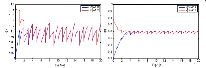
Figure 1 The dynamics of system (4) with two initial conditionsx(0) = 1,y(0) = 0.2 andx(0) = 1.2,
y(0) = 0.8.
Figure 2 The dynamics of system (4) with initial conditionx(0) = 1,y(0) = 0.2 but different impulsive effects.
Figure 3 The dynamics of system (4) with initial conditionx(0) = 1,y(0) = 0.5 but different cases of time delay.
density of the predator oscillates aroundx(t) = . and the population density of the prey oscillates aroundy(t) = ., this indicates the permanence of the system. The almost pe-riodic phenomenon is also easily observed from the figure. Moreover, we can see that the solutionU(t) = (x(t),y(t))Twith initial conditionx() = .,y() = . gradually approx-imate the other solution ofU(t) = (x(t),y(t))Twith initial conditionx() = ,y() = .,
and it proved that the almost periodic case is asymptotically stable.
From Figure , we can see that both the mean density population of the predator and the prey are decreasing with stronger impulsive effects, such as enhancing the harvesting rate, the efficiency of the insecticides for the species, and so on. In addition, in order to show the effects of the delays to the dynamics of the species, we consider two different cases of time delays, Case (withτ= .,τ= .,τ= .,τ= . in Figure (a)) and Case (withτ= .,τ= ,τ= .,τ= . in Figure (b)) with the same initial condition
x() = ,y() = .. We can see that the mean population density of the bigger time delays (Case ) is bigger that the smaller ones (Case ). This suggests that a longer digest delay in the predation may be conductive and could increase the possibility of the permanence of the population.
Competing interests
The authors declare that they have no competing interests.
Authors’ contributions
All authors contributed equally and significantly in writing this paper. All authors read and approved the final paper.
Acknowledgements
This work is supported by the National Natural Science Foundation of China (11372294, 51349011), Scientific Research Fund of Sichuan Provincial Education Department (14ZB0115, 15ZB0113), and Doctoral Research Fund of Southwest University of Science and Technology (15zx7138).
Received: 19 January 2016 Accepted: 28 June 2016
References
1. Holling, CS: Some characteristics of simple types of predation and parasitism. Can. Entomol.9, 385-398 (1966) 2. Hwang, J, Xiao, D: Analyses of bifurcations and stability in a predator-prey system with Holling type-IV functional
response. Acta Math. Appl. Sin.20, 167-178 (2004)
3. Peng, R, Wang, M: Positive steady states of the Holling-Tanner prey-predator model with diffusion. Proc. R. Soc. Edinb. A135, 149-164 (2005)
4. Hsu, SB, Hwang, TW, Kuang, Y: Global analysis of the Michaelis-Menten type ratio-dependent predator-prey system. J. Math. Biol.42, 489-506 (2001)
5. Beddington, JR: Mutual interference between parasites and predators and its effect on searching efficiency. J. Anim. Ecol.44, 331-340 (1975)
6. Kooij, RE, Zegeling, A: A predator-prey model with Ivlev’s functional response. J. Math. Anal. Appl.198, 473-489 (1996) 7. Hsu, SB, Hwang, TW, Kuang, Y: Global dynamics of a predator prey model with Hassell-Varley type functional
response. Discrete Contin. Dyn. Syst., Ser. B10, 857-875 (2005)
8. Crowley, PH, Martin, EK: Functional responses and interference within and between year classes of a dragonfly population. J. North Am. Benthol. Soc.8, 211-221 (1989)
9. Upadhyay, RK, Raw, SN, Rai, V: Dynamical complexities in a tri-trophic hybrid food chain model with Holling type II and Crowley-Martin functional responses. Nonlinear Anal., Model. Control15, 366-375 (2010)
10. Zhuang, K, Wen, Z: Analysis for a food chain model with Crowley-Martin functional response and time delay. World Acad. Sci., Eng. Technol.61, 562-565 (2010)
11. Ali, N, Jazar, M: Global dynamics of a modified Leslie-Gower predator-prey model with Crowley-Martin functional responses. J. Appl. Math. Comput.43, 271-293 (2013)
12. Liu, XQ, Zhong, SM, Tian, BD, Zheng, FX: Asymptotic properties of a stochastic predator-prey model with Crowley-Martin functional response. J. Appl. Math. Comput.43, 479-490 (2013)
13. Yin, HW, Xiao, XY, Wen, XQ, Liu, K: Pattern analysis of a modified Leslie-Gower predator-prey model with Crowley-Martin functional response and diffusion. Comput. Math. Appl.67, 1607-1621 (2014)
14. Zhang, H, Li, YQ, Jing, B, Zhao, WZ: Global stability of almost periodic solution of multispecies mutualism system with time delays and impulsive effects. Appl. Math. Comput.232, 1138-1150 (2014)
15. Liu, XX: Impulsive periodic oscillation for a predator-prey model with Hassell-Varley-Holling functional response. Appl. Math. Model.38, 1482-1494 (2014)
16. Joydip Dhar, D, Kunwer, SJ: Mathematical analysis of a delayed stage-structured predator-prey model with impulsive diffusion between two predators territories. Ecol. Complex.16, 59-67 (2013)
17. Shao, YF, Li, Y: Dynamical analysis of a stage structured predator-prey system with impulsive diffusion and generic functional response. Appl. Math. Comput.220, 472-481 (2013)
18. Pei, YZ, Li, CG, Fan, SH: A mathematical model of a three species prey-predator system with impulsive control and Holling functional response. Appl. Math. Comput.219, 10945-10955 (2013)
19. Yao, ZJ, Xie, SL, Yu, NF: Dynamics of cooperative predator-prey system with impulsive effects and Beddington-DeAngelis functional response. J. Egypt. Math. Soc.21, 213-223 (2013)
20. Yu, H, Zhong, S, Agarwal, P: Mathematics analysis and chaos in an ecological model with an impulsive control strategy. Commun. Nonlinear Sci. Numer. Simul.16, 776-786 (2011)
22. Sekiguchi, M, Ishiwata, E: Dynamics of a discretized SIR epidemic model with pulse vaccination and time delay. J. Comput. Appl. Math.236, 997-1008 (2011)
23. Wang, Y, Zheng, CD, Feng, EM: Stability analysis of mixed recurrent neural networks with time delay in the leakage term under impulsive perturbations. Neurocomputing119, 454-461 (2013)
24. Wang, C: Almost periodic solutions of impulsive BAM neural networks with variable delays on time scales. Commun. Nonlinear Sci. Numer. Simul.19, 2828-2842 (2014)
25. Zhao, HY: Existence and global exponential convergence of almost periodic solutions for cellular neural networks with variable delays. Chin. J. Eng. Math.22, 295-300 (2005)
26. Lakshmikantham, V, Bainov, DD, Simeonov, PS: Theory of Impulsive Differential Equations. World Scientific, Singapore (1989)
27. Bainov, DD, Simeonov, PS: Impulsive Differential Equations: Periodic Solutions and Applications. Longman, Burnt Mill (1993)
28. Samoilenko, AM, Perestyuk, NA: Impulsive Differential Equations. World Scientific, Singapore (1995)
29. Liu, Y, Zhao, SW: Controllability analysis of linear time-varying systems with multiple time delays and impulsive effects. Nonlinear Anal., Real World Appl.13, 558-568 (2012)
30. Wang, L, Yu, M, Niu, PC: Periodic solution and almost periodic solution of impulsive Lasota-Wazewska model with multiple time-varying delays. Comput. Math. Appl.64, 2383-2394 (2012)
31. Chen, L, Chen, F: Dynamic behaviors of the periodic predator-prey system with distributed time delays and impulsive effect. Nonlinear Anal., Real World Appl.12, 2467-2473 (2011)
32. Zhao, M, Wang, XT, Yu, HG, Zhu, J: Dynamics of an ecological model with impulsive control strategy and distributed time delay. Math. Comput. Simul.82, 1432-1444 (2012)
33. Tian, BD, Zhong, SM, Chen, N, Qiu, YH: Dynamical behavior for a food-chain model with impulsive harvest and digest delay. J. Appl. Math.2014, Article ID 168571 (2014)
34. Xiang, ZY, Long, D, Song, XY: A delayed Lotka-Volterra model with birth pulse and impulsive effect at different moment on the prey. Appl. Math. Comput.219, 10263-10270 (2013)
35. He, MX, Chen, FD, Li, Z: Almost periodic solution of an impulsive differential equation model of plankton allelopathy. Nonlinear Anal., Real World Appl.11, 2296-2301 (2010)
36. Zhang, TW, Li, YK, Ye, Y: On the existence and stability of a unique almost periodic solution of Schnoner’s competition model with pure-delays and impulsive effects. Commun. Nonlinear Sci. Numer. Simul.17, 1408-1422 (2012) 37. Zhang, H, Georgescu, P, Chen, L: An impulsive predator-prey system with Beddington-DeAngelis functional response
and time delay. Int. J. Biomath.1, 1-17 (2008)
38. He, CY: Almost Periodic Differential Equations. Higher Education Press, Beijing (1992)
39. Nakata, Y, Muroya, Y: Permanence for nonautonomous Lotka-Volterra cooperative systems with delays. Nonlinear Anal., Real World Appl.11, 528-534 (2010)