Numerical solutions of fractional wave equations using an efficient class of FDM based on the Hermite formula

R E S E A R C H

Open Access

Numerical solutions of fractional wave

equations using an efficient class of FDM

based on the Hermite formula

Mohamed M Khader

_{and Mohamed H Adel}

*_{Correspondence:}

[email protected] 1_{Department of Mathematics and} Statistics, College of Science, Al-Imam Mohammad Ibn Saud Islamic University (IMSIU), Riyadh, 11566, Saudi Arabia

2_{Department of Mathematics,} Faculty of Science, Benha University, Benha, Egypt

Full list of author information is available at the end of the article

Abstract

In this article, a numerical study is introduced for solving the fractional wave equations by using an efficient class of finite difference methods. The proposed scheme is based on the Hermite formula. The stability and the convergence analysis of the proposed methods are given by a recently proposed procedure similar to the standard von Neumann stability analysis. A simple and accurate stability criterion valid for different discretization schemes of the fractional derivative, arbitrary weight factor, and arbitrary order of the fractional derivative, are given and checked numerically. Finally, a numerical example is presented to confirm the theoretical results.

Keywords: finite difference methods; Hermite formula; fractional wave equation; stability and convergence analysis

1 Introduction

In recent years, it has turned out that many phenomena in engineering, physics, chem-istry, and other sciences can be described very successfully by models using mathemati-cal tools from fractional mathemati-calculus,i.e.the theory of derivatives and integrals of fractional (non-integer) order. There are many applications of the fractional differential equations (FDEs), see [–], and the studied models have received a great deal of attention like in the fields of viscoelastic materials [], solutes in natural porous or fractured media [], and anomalous diffusion. Most FDEs do not have exact solutions, so approximate and numer-ical techniques must be used [–]. Recently, several numernumer-ical methods to solve FDEs have been given such as the variational iteration method [], the Adomian’s decomposi-tion method [], the collocadecomposi-tion method [–], and the finite difference method [, , ]. In this section, we introduce the Riemann-Liouville definitions of the fractional derivative operatorDα_{[, ].}

Definition  The Riemann-Liouville derivativeDα_{of orderα of the functiony(x) is} de-fined by

Dα_{y(x) =} 

(n–α) dn dxn

x



y(τ)

(x–τ)α–n+dτ, x> ,α> , ()

wherenis the smallest integer exceedingαand(·) is the Gamma function. Ifα=m∈N, then the above definition coincides with the classicalmth derivativey(m)_(x).

In this paper, we will study the numerical solutions of the following fractional differential wave equation:

Dαu(x,t) =uxx(x,t) +f(x,t),  <α≤, () on a finite domain  <x<L, ≤t≤T, wheref(x,t) is the source term andDα _{is the} Riemann-Liouville derivative of orderαwith respect to the timet. Under the zero bound-ary conditions

u(,t) =u(L,t) = , ()

and the following initial conditions

u(x, ) =g(x) and ut(x, ) =g(x), ()

hereg(x) andg(x) are given functions.

In the last few years there have appeared many papers studying the proposed model ()-() [, ]. In this paper, we study the time fractional case and use an efficient class of finite difference methods based on the Hermite formula to solve this model.

The plan of the paper is as follows. In Section , we give some approximate formulas of the fractional derivatives and numerical finite difference scheme. In Section , we study the stability and the accuracy of the presented scheme. In Section , we introduce numerical solutions of fractional wave equation. The paper ends with some conclusions in Section .

2 Finite difference scheme of the fractional wave equation

In this section, we introduce an efficient class of FDM and use it to obtain the discretization finite difference formula of the time fractional wave equation (). For some positive integer numbersNandM, we use the notationsxandtfor the space-step length and the time-step length, respectively. The coordinates of the mesh points arexj=jx(j= , , . . . ,N), andtm=mt(m= , , . . . ,M) and the values of the solutionu(x,t) on these grid points areu(xj,tm)≡um_j U_jm, wherex=h=_NL,t=k=_MT.

For more details as regards discretization in fractional calculus see [, , ].

In the first step, the ordinary second order differential operators are discretized as fol-lows []:

∂_u

∂t

xj,tm =u

m+

j – umj +umj –

k +O

k. ()

Now, using equation (), we can derive an efficient approximate formula of the fractional derivative for ∂α

∂tαu(x,t) ( <α≤) at the points (xj,tm) as follows:

∂α

∂tαu(xj,tm) = 

( –α) tm



∂

∂tu(xj,s)(tm–s) –α

ds

= 

( –α) m

r= rk

(r–)k _ur+

j – urj+urj–

k +O

= 

( –α)( –α) m

r= _ur+

j – urj+urj–

k +O

k

× (m–r+ )–α– (m–r)–α k–α

= 

( –α)kα m

r=

ur_j+– ur_j+ur_j– (m–r+ )–α_{– (m–r)}–α

+ 

( –α) m

r=

(m–r+ )–α_{– (m–r)}–α_Ok–α_{. ()}

The above formula can be rewritten as

∂α_u(xj,tm)

∂tα =Aα,k m

r=

ω_r(α)um_j –r+– u_jm–r++um_j–r+ 

( –α)m –α

Ok–α

=Aα,k m

r=

ω_r(α)um_j –r+– u_jm–r++um_j–r+Ok, ()

where

Aα,k= 

( –α)kα and ω (α)

r =r–α– (r– )–α. ()

We must note thatω(rα)satisfies the following facts:

() ω(rα)> ,r= , , . . ..

() ωr(α)>ω(rα+),r= , , . . ..

Now, we are going to obtain the finite difference scheme of the fractional wave equation (). To achieve this aim we evaluate this equation at the points of the grid (xj,tm):

∂α

∂tαu(xj,tm) =

∂_u(xj,tm)

∂x +f(xj,tm). () Using equations () and (), we have

∂u(xj,tm)

∂x =Aα,k m

r=

ω_r(α)u_jm–r+– um_j –r++um_j–r–f(xj,tm) +Ok. ()

In order to get two additional equations, replacejbyj–  andj+ , respectively, in the above equation, so we have

∂u(xj–,tm)

∂x =Aα,k m

r=

ω(_rα)um_j––r+– u_jm_––r++u_jm_––r–f(xj–,tm) +O

k, ()

and

∂u(xj+,tm)

∂x =Aα,k m

r=

ω_r(α)um_j+–r+– u_jm_+–r++um_j+–r–f(xj+,tm) +O

The Hermite formula with two-order derivatives at the grid point (xj,tm) is with neglect the high order terms and under some simplifications, we can obtain the fol-lowing form: be the error, then we have the error formula



Proposition  Assuming that the solution of()has the form Tm

Proof Substitute in () byT_jm=ξmeiβjhand divide byeiβjh, we get

Using some trigonometric formulas and some simplifications we can obtain



from which we can obtain the required formula and this completes the proof.

3 Stability analysis

so,

which together with () completes the proof of the proposition.

Proposition  Assume thatξm (m= , , . . . ,M)is the solution of(),with the condition kα_< h

(–α),then|ξm| ≤ |ξ|(m= , , . . . ,M).

Proof It is easy to prove it by the mathematical induction together with Proposition .

Theorem  The finite difference scheme()is stable under the condition

kα< h 

Proof From Proposition  and (),Tm

≤ T,m= , , . . . ,M, which means that the

difference scheme is stable.

By the Lax equivalence theorem [] we can show that the numerical solution converges to the exact solution ash,k→.

4 Numerical results

In this section, we will test the proposed method by considering the following numerical example. Consider the fractional wave equation () in the interval [, ] with the following source term:

f(x,t) =

t–α_{(t+α– )}

( –α) +π 

sin(πx), ()

and the initial conditionsu(x, ) = ,ut(x, ) = –sin(πx).

The exact solution of equation () in this case isu(x,t) =sin(πx)(t_–t).

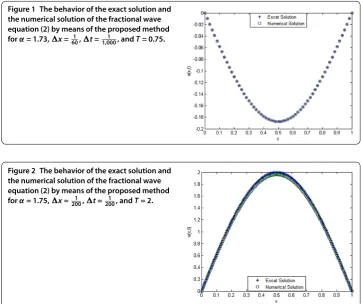
In Figures -, the behavior of the exact solution and the numerical solution of the frac-tional wave equation () by means of the fracfrac-tional finite difference method based on the Hermite formula with different values ofα,x,tand the final timeTis given.

From these figures, we can conclude that the numerical solution of the proposed method are in excellent agreement with the exact solution. Tables  and  show the magnitude of the maximum error between the exact solution and the numerical solution obtained by using the fractional FDM based on the Hermite formula discussed above with different values ofα,x,t, and the final timeT.

Figure 1 The behavior of the exact solution and the numerical solution of the fractional wave equation (2) by means of the proposed method forα= 1.73,x=₆₀1,t=_1,0001 , andT= 0.75.

Figure 2 The behavior of the exact solution and the numerical solution of the fractional wave equation (2) by means of the proposed method forα= 1.75,x= 1

200,t= 1

Figure 3 The behavior of the exact solution and the numerical solution of the fractional wave equation (2) by means of the proposed method forα= 1.66,x=₁₀₀1 ,t=₁₅₀1 , andT= 4.

Table 1 The maximum error with different values ofxandtforα= 1.5 andT= 0.2

x 1_{5 10}1 ₂₀1 ₃₀1 ₃₀1 ₄₀1 ₄₀1 ₄₅1

t ₅₀1 ₁₀₀1 ₁₅₀1 ₁₅₀1 ₂₀₀1 ₂₀₀1 ₂₁₀1 ₂₂₀1

max. error 0.01149 0.00361 0.00120 0.00115 0.00021 0.00019 0.00006 0.00004

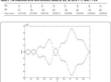
Table 2 The maximum error with different values ofx,tforα= 1.7 andT= 0.4

x ₁₀1 ₂₀1 ₃₀1 ₅₀1 ₅₀1 ₆₀1 ₆₀1 ₇₀1

t 1

50

1 100

1 200

1 250

1 300

1 400

1 450

1 480

max. error 0.01396 0.01064 0.00736 0.00653 0.00586 0.00494 0.00460 0.00443

Figure 4 The behavior of the numerical solution of the fractional wave equation (2) by means of the proposed method forα= 1.5,x=₁₅₀1 ,t=₁₂₀1 , andT= 2.

From Figure , we can see that the numerical solution is unstable, since the stability condition () is not satisfied.

5 Conclusion and remarks

for-mula. Special attention is given to the study of the stability and the convergence of the fractional finite difference scheme. To execute this aim we have resorted to a kind of frac-tional von Neumann stability analysis. From the theoretical study we can conclude that this procedure is suitable for the proposed fractional finite difference scheme and leads to very good predictions for the stability bounds. Numerical solutions and exact solutions of the proposed problem are compared and the derived stability condition is checked nu-merically. From this comparison, we can conclude that the numerical solutions are in ex-cellent agreement with the exact solutions. All computations in this paper were run with the Matlab programming package.

Competing interests

The authors declare that they have no competing interests.

Authors’ contributions

All authors contributed equally to the writing of this paper. All authors read and approved the final manuscript.

Author details

1_{Department of Mathematics and Statistics, College of Science, Al-Imam Mohammad Ibn Saud Islamic University (IMSIU),} Riyadh, 11566, Saudi Arabia.2_{Department of Mathematics, Faculty of Science, Benha University, Benha, Egypt.} 3_{Department of Mathematics, Faculty of Science, Cairo University, Giza, Egypt.}

Acknowledgements

The authors are very grateful for the editor’s and the referee’s careful reading and comments on this paper.

Received: 21 September 2015 Accepted: 20 December 2015

References

1. Bagley, RL, Calico, RA: Fractional-order state equations for the control of viscoelastic damped structures. J. Guid. Control Dyn.14(2), 304-311 (1999)

2. Baleanu, D, Diethelm, K, Scalas, E, Trujillo, JJ: Models and Numerical Methods, vol. 3. World Scientific, Singapore (2012) 3. Benson, DA, Wheatcraft, SW, Meerschaert, MM: The fractional-order governing equation of Lévy motion. Water

Resour. Res.36(6), 1413-1424 (2000)

4. Golmankhaneh, AK, Arefi, AK, Baleanu, D: Synchronization in a nonidentical fractional order of a proposed modified system. J. Vib. Control21(6), 1154-1161 (2015)

5. Gorenflo, R, Mainardi, F: Random walk models for space-fractional diffusion processes. Fract. Calc. Appl. Anal.1, 167-191 (1998)

6. Hilfer, R: Applications of Fractional Calculus in Physics. World Scientific, Singapore (2000)

7. Liu, F, Anh, V, Turner, I: Numerical solution of the space fractional Fokker-Planck equation. J. Comput. Appl. Math.166, 209-219 (2004)

8. Liu, F, Zhuang, P, Anh, V, Turner, I, Burrage, K: Stability and convergence of the difference methods for the space-time fractional advection-diffusion equation. Appl. Math. Comput.191(1), 12-20 (2007)

9. Lubich, C: Discretized fractional calculus. SIAM J. Math. Anal.17, 704-719 (1986)

10. Metzler, R, Klafter, J: The random walk’s guide to anomalous diffusion a fractional dynamics approach. Phys. Rep.339, 1-77 (2000)

11. Hristov, J: Approximate solutions to time-fractional models by integral balance approach. In: Cattani, C, Srivastava, HM, Yang, X-J (eds.) Fractals and Fractional Dynamics, pp. 78-109. de Gruyter, Berlin (2015) 12. Hristov, J: Double integral-balance method to the fractional subdiffusion equation: approximate solutions,

optimization problems to be resolved and numerical simulations. J. Vib. Control (2015). doi:10.1177/1077546315622773

13. Khader, MM, El-Danaf, TS, Hendy, AS: A computational matrix method for solving systems of high order fractional differential equations. Appl. Math. Model.37, 4035-4050 (2013)

14. Sweilam, NH, Khader, MM: A Chebyshev pseudo-spectral method for solving fractional integro-differential equations. ANZIAM J.51, 464-475 (2010)

15. Sweilam, NH, Khader, MM Adel, M: On the stability analysis of weighted average finite difference methods for fractional wave equation. Fract. Differ. Calc.2(1), 17-29 (2012)

16. Sweilam, NH, Khader, MM, Al-Bar, RF: Numerical studies for a multi-order fractional differential equation. Phys. Lett. A

371, 26-33 (2007)

17. Sweilam, NH, Khader, MM, Nagy, AM: Numerical solution of two-sided space- fractional wave equation using finite difference method. J. Comput. Appl. Math.235, 2832-2841 (2011)

18. Sweilam, NH, Khader, MM, Mahdy, AMS: Crank-Nicolson finite difference method for solving time-fractional diffusion equation. J. Fract. Calc. Appl.2(2), 1-9 (2012)

19. Sweilam, NH, Khader, MM, Adel, M: Weighted average finite difference methods for fractional order reaction-sub-diffusion equation. Walailak J. Sci. Technol.11(4), 361-377 (2014)

21. Yu, Q, Liu, F, Anh, V, Turner, I: Solving linear and nonlinear space-time fractional reaction-diffusion equations by Adomian decomposition method. Int. J. Numer. Methods Eng.47(1), 138-153 (2008)

22. Khader, MM: On the numerical solutions for the fractional diffusion equation. Commun. Nonlinear Sci. Numer. Simul.

16, 2535-2542 (2011)

23. Khader, MM, Hendy, AS: A numerical technique for solving fractional variational problems. Math. Methods Appl. Sci.

36(10), 1281-1289 (2013)

24. Khader, MM: On the numerical solution and convergence study for system of non-linear fractional diffusion equations. Can. J. Phys.92(12), 1658-1666 (2014)

25. Yuste, SB, Acedo, L: An explicit finite difference method and a new von Neumann-type stability analysis for fractional diffusion equations. SIAM J. Numer. Anal.42, 1862-1874 (2005)

26. Kilbas, AA, Srivastava, HM, Trujillo, JJ: Theory and Applications of Fractional Differential Equations. Elsevier, San Diego (2006)

27. Podlubny, I: Fractional Differential Equations. Academic Press, San Diego (1999)